
Optimization of the Bi-Axial Tracking System for a Photovoltaic Platform


Mechatronics and Environment, Department of Product Design, Transilvania University of Brașov, 500036 Brașov, Romania
Energies 2021, 14(3), 535; https://doi.org/10.3390/en14030535
Submission received: 17 December 2020
/
Revised: 17 January 2021
/
Accepted: 19 January 2021
/
Published: 21 January 2021
(This article belongs to the Special Issue PV Tracking Systems)
Abstract
:The article deals with the optimization of the azimuthal tracking mechanism for a photovoltaic (PV) platform, which uses linear actuators as actuation elements for both movements (diurnal and elevation). In the case of diurnal movement, where the platform’s angular field of orientation is large, a mechanism with a relatively simple structure is used for amplifying the actuator’s stroke and avoiding the risk of the system locking itself (by limiting the values of the transmission angle). The optimization study targets the mechanical device, the control device, and the bi-axial tracking program (embodied by the laws of motion in time for the platform’s diurnal and elevation angles) with the purpose of obtaining a high input of solar radiation, with a minimal energy consumption to achieve tracking. The study is carried out by using a virtual prototyping platform, which includes Computer Aided Design (CAD), Multi-Body Systems (MBS), and Design for Control (DFC) computer applications. The mechanical and control devices of the solar tracker are integrated and tested in mechatronic concept. The simulations’ results, which were performed for a set of representative days throughout the year, prove the effectiveness of the proposed design.
1. Introduction
Solar energy is one of the most important sources of renewable energy. There are two technologies that are used nowadays to produce electric power, Concentrated Solar Power (CSP) and Photovoltaic (PV) [1,2,3], the latter being addressed in this paper. Besides the amount of incoming solar radiation, the PV conversion’s efficiency depends on the type of solar cells as well as their temperature [4,5,6,7,8]. The solar radiation’s degree of capture can be maximized through the utilization of PV tracking systems (solar trackers), which can generate an increase in the conversion system’s efficiency by 20–50%, relative to the fixed (stationary) reference system, depending on the type of system (including its number of degrees of freedom—DOF), the control strategy, the location, and climate conditions. Just for the purpose of exemplifying, Table 1 shows a selection of data from literature, where the energy gain corresponds to either some representative days or entire year.
Depending on operating mode, solar trackers can be structured as follows: passive systems [15,16], in which the tracking movement is obtained usually by the thermal expansion of a fluid (liquid or gas) due to its heat sensitivity in a tube that is mounted on the PV module; active tracking systems [17,18,19], which are mechatronic systems based on devices that usually are electrically-driven.
Regarding the control system, one of the frequently used solutions is that based on photosensors (i.e., closed-loop control) [20,21,22,23,24], which, however, has the disadvantage that it can induce sun detecting errors in variable atmospheric conditions. The other commonly used solution is that based on predefined control algorithms (i.e., open-loop control), which can be accurately established on the basis of Earth–Sun astronomical system [25,26,27,28,29]. Lastly, by combining closed-loop and open-loop strategies, so called hybrid control systems are obtained [30,31,32].
Taking into account the number of degrees of freedom, two categories of tracking systems can be defined: mono-axial and bi-axial systems. Mono-axial systems allow the sun tracking on a single axis, which corresponds to either the diurnal movement or the elevation movement (case-by-case scenario) [33,34,35,36,37,38]. Bi-axial tracking systems allow the both movements, being able to ensure a high accuracy orientation throughout the year, which makes them more efficient than mono-axial systems [39,40,41,42,43,44].
According to the relative placement of the rotation axes, most existing bi-axial systems can fall into one of the following categories [25]: equatorial, pseudo-equatorial, azimuthal, and pseudo-azimuthal systems. The equatorial systems have as fixed axis the one of diurnal motion, which is parallel to the polar axis, while the elevation movement’s axis is variable depending on the diurnal axis. The fixed axis of the pseudo-equatorial systems is the elevation movement’s axis, which is placed horizontally, parallel to the East–West axis; the solution is obtained through the reversal of the axes’ order of rotation relative to the equatorial systems. The azimuthal systems have, as fixed axis, the diurnal movement’s axis, which is placed vertically, while the elevation movement’s axis varies depending on the diurnal axis. In pseudo-azimuthal systems, the fixed axis is also that of diurnal motion, but in this case it’s placed horizontally (parallel to the South–North axis).
Depending on the number of PV modules and their arrangement, the following configurations of tracking systems can be identified (Figure 1): tracking systems for separate PV modules: (a)—the modules are individually arranged and operated by their own motor sources; tracking systems for module strings: (b)—the modules are mounted individually, but oriented simultaneously by the same motor source(s) using motion transmission mechanisms (md—for diurnal movement, me—for elevation) [45]; platform tracking systems: (c)—the modules are mounted on the same support frame (platform type), and the motor source(s) orient the entire platform [46]; tracking systems for string platforms: (d)—the modules are mounted on individual strings, which are articulated to a common frame, the diurnal motion being performed as in a platform case [47]. In the schemes shown in Figure 1, each with two PV modules (noted PV 1 and PV 2), AA’/A1A1′/A2A2′ marks the diurnal motion axis, while BB’/B1B1′/B2B2′ is for the elevation motion axis, as the case may be.
Between the configurations that were presented, for reasons of cost and complexity of the kinematic scheme (reflected in the constructive solution), the most advantageous solution for tracking a group of PV modules is the one in Figure 1c, namely PV platform tracking system, which requires the minimum amount of motor sources to achieve bi-axial tracking (the drive element, which also integrates the electronic control device, being the most expensive component of a tracking system), without the usage of additional motion transmission mechanisms. This solution also has the advantage that it does not involve the risk of self-shading between modules, the modules’ layout thus being more compact than in other configurations whose design must ensure a certain distance between modules so that they do not overshadow each other. As a disadvantage, the mass load is higher than the ones found in all the other configurations, which can lead to significant driving forces (however, this deficiency can be limited by an adequate structure balancing).
By relating the configurations shown in Figure 1 to the basic types of bi-axial systems [25], the best suited solution for orienting a PV platform is the azimuthal system, and this is because, at least when referring to the diurnal motion, the platform can be arranged in such a way that the oriented structure’s center of mass is very close to the rotation axis, so the structure is well balanced, without needing additional balancing elements. This is reflected in low values of the actuators’ generated driving forces and, consequently, low energy consumption to achieve the tracking, even if the platform is large. The balance of the structure is still necessary in terms of elevation movement, otherwise high energy consumptions can result to achieve the orientation around this axis.
The active tracking systems’ actuation can be done with rotary motors or with linear actuators. If the motor source is of the rotating type (e.g., gear motor), a more compact system is obtained, which is able to ensure large angular strokes with no risk of the mechanism going into self-lock. However, the coupling embodiment solution is a little more complicated and the cost of such a motor is higher. Actuating with a linear actuator simplifies the constructive solution of the revolute joints (by which the orientation along the two axes is performed), at a lower cost. In this case, the disadvantage is that for achieving large angular amplitudes, a high linear stroke actuator is required, and there’s also the risk of the mechanism going into self-lock. The issue can be solved by inserting a stroke amplification mechanism between the linear actuator and the element to be oriented. If chosen and placed judiciously, this can bring important benefits from a functioning point of view, without significantly raising the tracking system cost.
In these terms, the main purpose of the present paper is to optimally design and test an innovative azimuthal bi-axial tracking system for a PV platform, which is able to avoid the deficiencies of some existing solutions (partly mentioned above, others following to be indicated in the next section of the paper), and it assures a better efficiency and tracking accuracy (as the results of the numerical simulations will demonstrate). The proposed bi-axial solar tracker uses as driving elements two linear actuators identical in type-dimensions. Solar tracker design started from the requirement that the system has to be able to ensure the orientation and positioning of the platform in the maximum angular fields, both for the diurnal and the elevation movement. Although there is a significant difference between the two angular domains (double angular range during diurnal movement compared to elevation), through the proposed system it is possible to use the same type of actuator for both movements (namely a linear stroke actuator with relatively small dimensions) by introducing a stroke amplification mechanism for diurnal motion, a mechanism that has a simple kinematic scheme and structure, which does not raise problems related to the angular capacity of the joints nor does it present a risk of self-locking at high strokes.
The proposed tracking system is optimized both in terms of the mechanical device and the control device (including the bi-axial tracking program, embodied by the laws of motion in time for the diurnal and elevation angles of the platform), so as to obtain a high input of incident solar radiation (which translates into maximizing the amount of electricity produced by the PV platform) with minimum energy consumption necessary to achieve the bi-axial tracking of the platform. In this regard, the optimization process targets the following design objectives: minimization of driving forces generated by linear actuators to achieve tracking, minimization of tracking errors (as differences between positioning angles imposed on the platform by the bi-axial tracking program and the current angles achieved by the mechatronic system), maximization of energy gain by designing a step-by-step tracking program whose efficiency is very close to that of the ideal tracking case, when the platform would be oriented with continuous movement throughout the day (this is not used in practice due to issues that will be mentioned later). The algorithm for optimizing the bi-axial tracking program is an original one, taking into account both the energy produced by the PV system and the one consumed to achieve the orientation, all the defining parameters of the diurnal and elevation motion laws being considered as design variables. To the best of our knowledge, it is the first time that the tracking program design is approached in such a comprehensive way.
A virtual prototyping platform, which includes CAD (Computer Aided Design)—CATIA, MBS (Multi-Body Systems)—ADAMS and DFC (Design for Control)—EASY5 software solutions, was used to design and test the proposed tracking system, as will be depicted in the following sections.
2. Designing the Tracking System’s Mechanical Device
As mentioned earlier, the main issue with azimuthal tracking systems that are driven by linear actuators is the need to use relatively large stroke actuators (hence also dimensions) to ensure the angular range of diurnal motion (180°, from the position with the platform facing East to the one facing West). At the same time, there’s a risk that the system will self-lock due to the transmission angle between the actuator’s piston and the mobile part of the support pillar. Another issue that must be avoided is that of the impact (strike) between the piston and the pillar.
In designing the azimuthal tracking mechanism brought forward in this paper, it was started from the premise of using actuators with identical specifications for both degrees of freedom (even if it exists a large difference in the platform’s angular orientation on the two rotation axes), namely an actuator that would not have a very large stroke (it would be more suitable for the elevation movement). In order to ensure such a requirement, it’s necessary to design a mechanism for amplifying the actuator’s stroke for diurnal motion, interposed between the actuator’s piston and the mobile part of the support pillar; this mechanism would make it possible to perform the azimuthal orientation range (theoretically, 180°) with a reasonable stroke of the actuator (not much higher than that of the actuator for altitudinal motion, where the maximum range is practically half) and without generating a risk of self-locking or impact between various parts of the system.
Mechanical systems for stroke amplification can be based on various mechanism topologies, such as those presented in [46,48,49,50]. To simplify the constructive solution, ensure motion continuity and safety in operation (even in the presence of non-stationary external disturbances, e.g., wind) it’s preferable to avoid mechanisms that have profiled elements (e.g., gears, belt, or chain), so the best suited solution is the one based on an articulated bar mechanism (linkage). For example, the solution in Figure 2 uses a spatial four-bar linkage (DEFG) to amplify the actuator’s stroke from the diurnal motion of an azimuthal tracking system [46]. Such a mechanism includes two spherical joints at the ends of the connecting rod (E, F), and it is likely that angular capacity issues of these joints will pop up, which could generate wear, shocks or even functional locks [51,52]. At the same time, a fairly large space is required for the mechanism to function.
The solar tracker proposed here includes in diurnal motion subsystem a planar slider—rocker mechanism for amplifying the actuator’s stroke, whose piston acts on the slider (push—pull), while the rocker is connected to the vertical support pillar’s mobile part. The proposed mechanism does not present any risk related to the joints’ angular capacity and the occupied space (volume) is quite small; there’s also the advantage that the mechanism can be mounted at ground level. For the elevation (altitudinal) motion, where the angular range of motion is smaller, it was opted for a classic solution, to which the piston is connected on the platform’s frame, while the cylinder is articulated on the pillar’s mobile part. The tracking system thus defined is schematically represented in Figure 3, separated on the two kinematic contours corresponding to the azimuthal and altitudinal motions (the representations are made in normal planes to the axes of the actuators’ rotational joints).
The proposed solar tracker contains the following components: the mechanism’s base (1), which includes the fixed part of the pillar or pole (1′); 8 mobile bodies: the cylinder (2) and the piston (3) of the diurnal motion’s actuator, the slider (4), the connecting rod (5) and the rocker (6) of the stroke amplification mechanism, where the rocker is common part with the moving part of the pole (6′), the cylinder (7) and the piston (8) of the elevation motion’s actuator, the platform (9), which includes the PV modules and the support frame; 3 revolute joints: A (connected bodies: 2–1), C (3–4), E (4–5), F (5–6), G (6–1′); H (7–6′), J (8–9), K (9–6′), and 3 translational joints: B (2–3), D (4–1), I (7–8).
Based on the structural schemes in Figure 3, the tracking system’s CAD model was designed using the specialized CATIA software. Subsequently, the solid body models were exported for later import into ADAMS. The MBS model of the tracking systems presented in Figure 4 is finalized through the usage of the general ADAMS/View preprocessing module, with modeling both geometric (joints) and kinematic (drivers) constraints.
The actuators used to drive the two motions are of the ELERO ATON-2 type, from size class “2” (compressed size—1275 mm, maximum stroke—600 mm), which ensures irreversibility of the motion in stationary positions (between drives). The 8 PV modules of the Helios Energy Europe (HHE) type are placed on the platform, with an active area of 1.638 m2 (13.104 m2 for the entire platform) and an average conversion efficiency of 14%.
As mentioned, the azimuthal mechanism configuration requires rigorous balancing in the elevation movement subsystem (otherwise, the power or energy consumption to perform this motion can be quite significant). In this regard, a pair of two counterweights that are connected to the platform frame was used in the proposed solution, counterweights that are symmetrically arranged relative to the transverse—vertical (YZ) plane containing the support pillar’s axis. The counterweights’ positioning and sizing was made in such a way that the assembly’s center of mass is as close as possible to the rotation axis for the elevation motion.
The actuators have been preliminary modeled through kinematic restrictions that control the relative motions between the actuators’ components. In fact, it was started from controlling the motions in the revolute joints G and K, thus imposing the platform’s angular positions on the two axes of rotation. Subsequently, through the inverse kinematics, the laws of motion in the translational joints of the actuators (B and I) are determined. For example, the correlation between the platform’s angles and the actuator’s strokes is shown in Figure 5 (the duration of the simulation is not relevant in this case; a one hour interval was chosen), considering the maximum angular ranges of motion of the platform (ψ*—the diurnal angle, in joint G; α*—the elevation angle, in joint K): ψ*∈ (90°, −90°), α* ∊ (0°, 90°). For the diurnal motion, the limit values correspond to the positions in which the platform faces East (ψ* = 90°) and West (ψ* = −90°), by relating the angle to the noon reference position (when ψ* = 0°). For the elevation motion, the angles’ limit values are those in which the platform is vertical (α* = 0°)—position that is recommended in strong wind conditions, respectively, horizontal (α* = 90°)—recommended position in cloudy sky conditions, for maximum capture of the diffuse component of solar radiation.
The two end (limit) positions of the tracking mechanism/platform, defined by the angle pairs ψ* = 90° (platform facing East), α* = 0° (platform vertically) and ψ* = −90° (facing West), α* = 90° (horizontally), are represented in Figure 6 (the horizontal axis of this representation is the East–West axis). In the two positions, the linear actuators (i.e., the drivers) are in the following states (La is the actuator’s length, |AC| or |HJ|, by case): (a) diurnal motion actuator—fully compressed (La = 1275 mm), elevation motion actuator—extended (La = 1645.78 mm); (b) diurnal motion actuator—extended (La = 1866.79 mm), elevation motion actuator—fully compressed (La = 1275 mm).
Both the diagrams in Figure 5 and the graphical simulation frames in Figure 6 show that the chosen type of actuator provides the necessary strokes for the two motions. This is the result of a complex optimization study that was carried out in ADAMS, as it will be described below. The optimization aimed at establishing the optimal disposal of the two actuating sources, and the positioning or sizing of the slider-rocker mechanism used to amplify the stroke for the diurnal movement.
The optimal design was carried out separately on the kinematic contours (subsystems) corresponding to the two motions (ABCDEFG for diurnal motion and HIJK for elevation). The optimization problem for each subsystem is of mono-objective type, which is achieved by following the next steps: model parameterization, modeling of the design variables, modeling of the objective function to be optimized, modeling of the design constraints, the actual optimization.
The parameterization of the model, which allows the automatic modification (repositioning, reorientation, and resizing, as appropriate) of the objects in the model (e.g., bodies, joints, force-generating elements) by creating “master-slave” type relations, was done by using the design points (the joints’ locations), by automatically generating expressions that control the location and the orientation of the objects once they are modeled by reference to the respective points. In addition, for the complete parameterization of the mechanism, some manually created expressions were needed (by using the expression modeling module in ADAMS—Expression Builder).
The design points’ coordinates are subsequently defined as independent design variables. Of the 33 coordinates of the 11 design points (7 points in the diurnal motion subsystem and 4 points in the elevation subsystem), only some are considered design variables, the others being established either exclusively on constructive considerations or dependent on the coordinates of other design points or variables, as follows:
- global coordinates of points A and C, where the connections of the diurnal motion actuator are located (A—cylinder joint at base, C—piston joint at slider), are defined as design variables (DV):XA→DV_1, YA→DV_2, ZA→DV_3; XC→DV_4, YC→DV_5, ZC→DV_6;
- point B, representing the location of the translational coupling between the two parts of the actuator (piston and cylinder), is modeled along axis defined by points A and C, at half the distance between the points, using the expression:where LOC_ALONG_LINE (Object for Start Point, Object for Point on Line, Distance) is a predefined function ADAMS that returns the location that is distance from frame start point (A) toward point on line (C), while predefined function DM (Object 1, Object 2) returns the magnitude of the distance between the two points;LOC_ALONG_LINE (A, C, DM (A, C)/2),
- point E’s coordinates, representing the location of the revolute joint between slider and rod of the stroke amplification mechanism, are established considering the requirement that the slider be placed in the direction of the projection in the XY plane of the actuator axis:where length lp = |CE| is an imposed parameter, and is the actuator’s position angle in the XY plane (measured against the X axis);XE = XC + lp ⋅ cos θ, YE = YC − lp ⋅ sin θ, ZE = ZC,
- the location of point D, where the translational joint between slider and the base of the mechanism is placed, is determined at half the distance between points C and E (as a position in the XY plane), and at the base level (as a position on the vertical axis Z):
- the location of point F, where the revolute joint between the connecting rod of the stroke amplification mechanism and the mobile part of the pillar is placed, is established as a vertical position at the same level as the E joint, while the coordinates on the X and Y axes are considered design variables:XF→DV_7, YF→DV_8, ZF = ZE;
- the coordinates of point G, representing the location of the revolute joint between the pillar’s mobile and fixed parts (through which the diurnal orientation of the platform is achieved), are established on constructive reasons;
- the locations of points H and J, where the actuator’s joints are placed for the elevation motion to the adjacent elements (H—cylinder’s joint at the mobile part of the pillar, J—piston’s joint at the platform), are established as position on the longitudinal axis X at the same level with the joint or point G (the actuator will be arranged in the transverse-vertical plane containing the axis of the pillar), while the coordinates on the Y and Z axes are considered design variables:XH = XG, YH→DV_9, ZH→DV_10; XJ = XG, YJ→DV_11, ZJ→DV_12;
- point I, representing the location of the translational joint between the actuator’s piston and cylinder, shall be modeled in the direction of the axis defined by points H and J, at half the distance between the points, using the expression:with a similar significance to the one in expression (2);LOC_ALONG_LINE (H, J, DM (H, J)/2),
- the coordinates of point K, representing the location of the revolute joint between the platform and the mobile part of the pillar (through which the altitudinal orientation of the platform is achieved), are established on constructive reasons.
The above presented design variables and expressions control the locations of the couplings in the initial (modeling) configuration; during the mechanism working, they change according to the kinematics of the tracking system. Therefore, in the optimization process of the bi-axial mechanism, 12 independent design variables are used, 8 of which in the diurnal motion contour, and 4 in the elevation motion contour. Each variable is defined by its initial value, along with a domain expressed by boundaries (min, max) in which the optimal value of the variable is looked for.
As an objective function, for each motion subsystem, the actuator driving force for generating the angular movement field of the platform was considered (this is reflected in the power or energy consumption required to achieve tracking); the purpose of optimization consists from the minimization of the root mean square (RMS) of this variable force over time.
The optimization process complexity is mainly given by the multiple design constraints that have been taken into account so that the achievement of the optimization objective (minimizing the driving force) is accompanied by the functional and constructive rationality of the obtained solution, still considering previously mentioned requirements: usage of a certain type of actuator (defined by minimum length in compressed state and the maximum stroke it can achieve); avoidance of the risk of the mechanism going into self-lock by considering a safety margin regarding the value of the transmission angle (marked for the two motion subsystems in Figure 7); avoidance of the impact between the parts of the mechanism. Each constraint generates an inequality relation, keeping the constraint value less than or equal to zero in the optimization process (in other words, the positive value of the constraint would be equivalent to violating it, and such a design is unacceptable).
In this regard, the following design constraints (DC) have been considered or modeled:
- respecting the actuator’s minimum length (in compressed state): DC_1 = 1275 mm − La, where La is the actuator’s current length (La = |AC| or La = |HJ|);
- respecting the actuator’s maximum stroke (thus length): DC_2 = La − 1875 mm;
- avoiding the self-locking of the mechanism by keeping the transmission angle within rational boundaries (although in theory self-lock occurs when τ = 0° and τ = 180°, in practice this can occur before those values have been achieved, especially because of friction, which is why a safety limit of 15° was considered): DC_3 = 15° − τ, and DC_4 = τ − 165°;
- avoiding impact between bodies (penetrations and strikes between their geometrical shapes), considering only the pairs of bodies that do present a risk of impact (see the next paragraph): DC_5 = CONTACT(CONTACT_1, 0, 1, 0), DC_6 = CONTACT(CONTACT_2, 0, 1, 0), DC_7 = CONTACT(CONTACT_3, 0, 1, 0), DC_8 = CONTACT(CONTACT_4, 0, 1, 0).
For modeling the last four constraints, the CONTACT (Contact Name, On Body, Component, Axes) predefined function was used, which returns by the Component argument (when Component = 1) the magnitude of the force applied by all incidents of contact (Contact Name) between two bodies “i–j” (CONTACT_1: diurnal motion actuator piston—slider, CONTACT_2: stroke amplifying mechanism rod—pillar, CONTACT_3: elevation motion actuator cylinder—pillar, CONTACT_4: elevation motion actuator piston—platform), measured on body i/j (On_Body = 0/1) and expressed relative to the global coordinate system (Axes = 0).
Therefore, in each of the two motion subsystems, 6 constraints were modeled, namely DC_1–DC_6 in the diurnal motion subsystem, respectively DC_1–DC_4, DC_7, and DC_8 in the elevation subsystem. For each constraint, the maximum value is monitored during the simulation, considering that if this value is kept negative, any other value during the simulation can only be negative.
The actual optimization, which aims to minimize the design objective’s value while respecting the constraints, was carried out by using an algorithm provided with ADAMS/View (namely, OPTDES-GRG). The study was performed considering the maximum platform revolute domains, ψ* ∊ (90°, −90°) and α* ∊ (0°, 90°), the duration of the simulation for each subsystem being one hour, with continuous motion (step-by-step tracking during daylight will be addressed in Section 4). Following the optimization process, the variation charts of the design constraints in the two subsystems of the mechanism (I—diurnal motion, II—elevation motion) are shown in Figure 8. One can see that the constraints DC_1–DC_4 remain negative throughout the simulation, while DC_5–DC_8 are null (no impact between bodies), so the requirements regarding the functioning of the mechanism and the rationality of the constructive solution are met. Figure 8 also shows the variations of the driving forces generated by the linear actuators, with reasonable or reduced values during the simulation in both subsystems (in the elevation motions’ case, this is mainly the effect of the proposed counterweight balancing system, otherwise the required driving force, and therefore energy consumption, would have been much higher).
3. Designing the Control System
Among the control variants summarized in the introductory section, for the proposed bi-axial azimuthal tracking system, an open-loop control strategy was chosen, based on a predefined tracking program (whose design will be detailed in the next section of the paper). In order to design the control system, a specialized DFC computer application (namely, EASY5) was used in conjunction with the MBS software (ADAMS), in co-simulation mode, which is based on the input and output plants (outputs describe parameters submitted to EASY5, while inputs describe returned parameters in ADAMS). The communication between the MBS and DFC models is managed by using ADAMS/Controls, a plugin to ADAMS/View, which allows connecting mechanical models developed in ADAMS/View with control system models from specific DFC applications.
Depending on the number of monitored or controlled parameters, various control schemes can be designed, with one (usually for position), two (position and speed), or three (position, speed and current) loops. Multi-loop systems define so-called cascade control scheme (for example, two-loop systems use the main and external controller output to control the secondary and internal controller input), thus ensuring higher performance (stability, robustness).
For this work, it was selected a control scheme with two loops (for both the diurnal and elevation motions), the controlled parameters being the platform’s angles and the linear speeds in the actuators. Several control variants (single-loop, multi-loop) were tested, the chosen solution being the one that ensures the best ratio between the complexity and the performance of the system. For this control system configuration, the communication diagram between the MBS (ADAMS) and DFC (EASY5) models is the one shown in Figure 9, in which: OUT-1—the measured or current angle of the platform, OUT-2—linear speed in the actuator, IN—driving force developed by the actuator. The tracking system being of bi-axial type (with two linear actuators), the general control scheme will in fact include two schemes like the one in Figure 9 (one for each motion of the platform).
Input and output parameters were modeled in ADAMS using predefined functions. The input variable (IN) receives the current value from the control system, so that it is initially modeled in ADAMS with the value 0.0, being assigned to the driving force in the actuator by the predefined function Variable Value (VARVAL). For the output variable, OUT-1 (representing the diurnal or elevation angle, as appropriate), the corresponding function provides the angular position of the platform, for the modeling of which the predefined function AZ(From Marker, To Marker) was used. The coordinate system markers are placed on the adjacent bodies in the revolute joints through which the orientation of the platform around the two motion axes is performed.
For the output variable OUT-2 (representing the linear speed in the actuator), the time function returns the relative displacement between the actuator’s piston and cylinder, the modeling being performed with the predefined function VZ(From Marker, To Marker), in which the coordinate systems are positioned in the translational joint between the actuator’s elements.
The control system model conceived in EASY5 (Figure 10) contains the following types of components: RF—input function generator, used to model the imposed angle (diurnal or elevation); SJ—summation block, used to compare the input signals (e.g., the imposed “+1” angle with the measured “−1” angle); LA—block for modeling the control element (controller); MSC.ADAMS—interface block that establishes the connection with the MBS model developed in ADAMS.
The position and velocity controllers were modeled by using low pass filters. In EASY5, this controller can be modeled through a First Order Lag (LA) block, which generates a continuous transfer function in constant time format, as follows (EASY5 notations are used):
where: S_In—controller input, S_Out—controller output, GAI—amplification factor, TC–response time constant.
Controllers’ tuning consists in establishing the optimal values of their amplification factors. This was carried out by implementing a parametric optimization procedure in ADAMS, such as the one presented in the previous chapter of the paper. In this regard, the control system model was transferred from EASY5 to ADAMS as an External System Library (ESL) file, and subsequently the amplification factors of the controllers were defined in ADAMS as design variables.
The optimization goal consists in minimizing the tracking error (in terms of root mean square), which defines the deviation between the imposed and measured values of the platform’s angles (diurnal or elevation, by case). In the control system model shown in Figure 10, the tracking error is materialized by the output from SJ1 and respectively SJ3 block. By minimizing these errors, the conditions are ensured so that there are no losses of incidental solar radiation due to possible errors in the positioning of the platform, by reference to the imposed tracking program. As mentioned, the design variables for optimizing the control system are represented by the amplification factors of the controllers (GAIp—position controller, GAIs—speed controller), for each of the two motions of the tracking system.
The optimization problem of the control device, which is one of mono-objective type, was carried out by using the same algorithm as for the optimal design of the mechanical model of the bi-axial solar tracker (OptDes-GRG). Numerical simulation is performed by considering a motion or tracking step with the amplitude of 20°, which is covered in 30 s, for both movements. Following the optimization process, the following values of the amplification factors have been obtained: the controller for diurnal movement—GAIp = 2392, GAIs = 2349; the controller for elevation movement—GAIp = 3648, GAIs = 3516. With these amplification factors, there result insignificant values of tracking errors (in terms of root mean square—RMS), namely RMS = 8.151 × 10⁻⁶ for diurnal motion, and RMS = 9.546 × 10⁻⁶ for elevation, which ensures accurate tracking of the imposed motion laws (hence, the optimal incidence of sunrays on the platform’s surface).
Next, the robustness of the designed control system is checked. Robustness is the ability of the system to operate at or near imposed performance indices when one or more parameters of the model change, or when external disturbances affect the system. In this case, the robustness of the diurnal motion’s control system shall be checked at the occurrence of a non-stationary external disturbance represented by the action of wind. A gust of wind which acts during the tracking step (20° traveled in 30 s) and that generates a loading torque of 60 Nm at the level of the revolute joint between the mobile and fixed parts of the support pillar is considered. This load corresponds to the maximum value of the wind speed registered in the Brașov area (namely, 15 m/s) during a 3-year monitoring (climatic data recording) [53].
The profile of the wind gust is presented in Figure 11a, the sign of the generated torque depending on the wind’s direction, front or rear relative to the platform (the torque is therefore either “+” motor or resistant ”−”, related to the platform’s direction of movement). The variation of the tracking error during the wind’s action is insignificant (the maximum amplitude being about 3.5 × 10⁻⁵), and subsequently the system stabilizes accordingly, as can be seen in Figure 11b. Similar results were obtained for the elevation motion as well, thus confirming the ability of the proposed control system to compensate very well for the effect of non-stationary external disturbances.
4. Designing the Bi-Axial Tracking Program
In order to optimally design the bi-axial tracking program, a mathematical model for determining the energy production of the PV platform had to be developed and subsequently transposed or implemented in the tracking mechanism’s MBS model done in ADAMS through the usage of the ADAMS/Function Builder module. Thus, it’s possible to assess both the energy produced by the PV tracking system and the energy consumed to achieve the orientation around the two axes.
As is well known, solar radiation is composed of three components: direct, diffuse, and reflected. Solar radiation is influenced by the geographical location, the relief configuration, season, time of day, climatic conditions (clouds, rain, air clarity), and the level of pollution in the area. To design and implement a PV plant, the amount of solar radiation is estimated, either using meteorological databases (such as Meteonorm) or by empirical models based on measurements.
The literature presents various models for establishing the quantity of solar radiation (global or component-based) [54,55,56,57,58]. For the present work, the empirical model developed by Meliss [59] (which is close to the climatic conditions in the Brașov area) is used for modeling solar radiation. For simplicity’s sake, it’s considered only the direct radiation, starting from the premise that the sky is clear (cloudless).
Sunray’s altitudinal angle (which is formed between the sunray and the area’s horizontal plane) is given by the following equation:
in which: ϕ—the latitude (45.65° for Brașov area), ω—the hour angle, δ—the declination angle. The angles of the equatorial orientation (ω, δ) are modeled according to the equations presented in [60], depending on the solar time and the day number (e.g., N = 172 for 21 June, the summer solstice day).
Sunray’s diurnal angle for the azimuthal orientation (ψ) is expressed by the equation:
where sgn ω is the hour angle sign (negative before noon, positive in the afternoon).
The incident solar radiation can be established according to the amount of direct radiation (GD) and the incidence angle (i),
In the azimuthal setup, the incidence angle is determined as follows:
where ψ* and α* are the angles of azimuthal orientation of the PV platform, as shown in Figure 12. The platform’s diurnal angle is considered positive (ψ*+) in the morning and negative in the afternoon, the reference (ψ* = 0°) corresponding to the platform layout at noon, when it faces South. The reference position for the elevation angle (α* = 0°) is the one in which the platform is vertical, the angle being positive (α*+) for clockwise rotation.
There are two way to ensure the sun tracking, with continuous movement or step-by-step. The ideal case is that of continuous orientation throughout the daylight, so that the normal to the platform coincides at all times with the direction of the sunray. To ensure the ideal incidence, the platform’s orientation angles must coincide with the sunray’s angles (ψ* = ψ, α* = α). For example, Figure 13 shows the incident radiation (coinciding with that of direct radiation) for continuous tracking (I) on the day of summer solstice, along with the curve corresponding to the fixed or stationary system (II), at which the platform is maintained throughout the entire day in the noon position (ψ* = 0°), at an elevation angle equal to that of the sunray at that time (α* = 67.8°).
However, continuous tracking generates quite some known issues, as follows: long running time (corresponding to daylight duration), large transmission ratios (the speed with which the sun tracking is made is really low), possible unstable behavior of the system in case of being acted on by non-stationary disturbances (e.g., wind). Because of these issues, step-by-step tracking is frequently used in practice, for both the diurnal motion and the elevation one, even if it’s less efficient when it comes to capturing solar radiation. However, through optimal design of the laws of motion in steps, it is possible to achieve a high efficiency of stepping tracking, comparable to that of continuous movement tracking. The optimization of the azimuthal tracking program aims to correlate the two movements of the platform, expressed by the diurnal and elevation angles, so as to result in an optimal incidence of sunrays on the platform surface.
The parameters that define the stepping movement law will be treated as variables in the optimal design process of the tracking program, as follows: the angular movement range (in which the platform is oriented), the tracking steps number and size, the operating and running time (defined by time intervals in which the system is operated). There are certain interdependencies between the mentioned variables, for example the sum of the movement steps’ sizes equals the amplitude of the angular movement range. By optimally correlating the data, a step-by-step law of motion can be obtained that’s close in efficiency to the continuous movement.
The solar radiation curve is symmetrical, relative to the solar noon (see Figure 13), which is also transposed on the tracking law. Thus, the process of optimally designing the tracking law is simplified, by considering only half of law, from sunrise to noon, which is subsequently adapted for the other half of the law, from noon to sunset (e.g., reversing the diurnal angle sign).
The laws of motion for the azimuthal solar tracker (corresponding to the diurnal and elevation angles), have been defined with the help of the ADAMS/Function Builder module by summing STEP functions, as follows:
in which: x—the independent parameter (i.e., time), x0/xk−1—independent parameter’s value at the beginning of the function, f0/fk−1—function’s initial value, x1/xk—independent parameter’s value at the end of the function, f1/fk—function’s final value. It should be noted that starting with the second STEP function, the value of the current function is expressed in relation to the previous one.
Thus, the half-law tracking functions have been expressed in the following way:
- diurnal motion (Figure 14):where: tr—sunrise time, td1—beginning time for the first step, in relation to the sunset time; td2—beginning time for the second step, in relation to the beginning of the first step; tdk—beginning time for the last step, in relation to the beginning of the previous one; Δt—motion steps duration (for simplicity, the same duration was considered for all the steps); ψ0—initial value of diurnal angle; Δψ1—size of first motion step; Δψ2—size of the second step; Δψk—size of the last step (before noon—tn);
- elevation motion (Figure 15):where the significances of the parameters correspond to those of diurnal movement, considering that the motion steps’ duration is the same with the one from diurnal movement.
As mentioned, the purpose of the process of optimizing the laws of motion consists of maximizing the PV system efficiency, that is expressed through the following function:
in which: ET—energy production of the PV platform with bi-axial tracking, EF—energy production of the equivalent stationary platform, EC—energy consumption to achieve the bi-axial orientation.
The energy production of the PV platform (with bi-axial tracking or fixed) is determined according to the platform’s surface, the PV modules’ yield, and the area of the region delimited by the incident radiation graph, while the energy consumed for tracking depends on the driving forces and the linear speeds in the actuators [25].
In the optimization process of the bi-axial tracking program, two design constraints have been defined, which refer to the fact that the final or last steps in the half of laws for the diurnal and elevation movements have to be completed before noon, according to the models shown in Figure 14 and Figure 15. The two design constraints (C1—for the diurnal movement law, and, respectively, C2—for the elevation movement law) create inequality relations, the optimization process keeping the negative values, null at limit (otherwise, for positive values, the constraints are considered to be violated), as follows:
Thus, the optimization of the optimization program aims to determine the design variables’ values (ψ0, k, Δψ1, Δψ2, ..., Δψk, td1, td2, ..., tdk; α0, j, Δα1, Δα2, ..., Δαj, te1, te2, ..., tej) that ensure maximizing the objective function (F) while respecting the design constraints (C1, C2). It should be mentioned that the duration of the motion and tracking steps was not considered a design variable for the optimization process, it being an imposed parameter (same value for both motions, Δt = 0.5 min).
The number of tracking steps for half-laws (k—diurnal movement, j—elevation movement), actually determines the number of variable pairs Δψ1...k–td1...k/Δα1...j–te1...j of the tracking program, in other words the number of STEP functions from Equations (14) and (15). To make automatic updating possible in the process of optimizing the laws of motion depending on the number of steps, a conditional function (the predefined IF function in ADAMS/Function Builder) was used, with the following syntax:
in which: Expression—the expression that is evaluated, E1—the returned expression if the value of the evaluated expression is negative, E2—the returned expression if the value of the evaluated expression is zero, E3—the returned expression if the value of the evaluated expression is positive.
IF (Expression: E1, E2, E3),
For example, if it is considered that the range of variation of the variable representing the number of steps for diurnal movement is k ∊ (1, 3), the corresponding tracking law will take the following form:
in which:
If for the same variable it is considered that k ∊ (1, 2), Equation (19) becomes:
the evaluated expression cannot return a positive value in this case (so the “0” value is used to make up for the lack of expression E3), while for k ∊ (1, 4) a cascade configuration of IF functions is required, as follows:
in which
expressions E1, E2, and E3 having the forms according to Equation (20).
The actual optimization is performed with the same algorithm used in the previous sections of the work for the mechanical and control models, namely OPTDES-GRG with the Forward differentiation method.
After determining the optimal values of the design variables for half a law (from sunrise to noon), the transposition is made for the interval from noon to sunset, symmetrical with respect to the noon position, thus obtaining the tracking law for the entire daylight (from sunrise to sunset). With regards to the energy consumed to achieve the bi-axial orientation of the platform, the return diurnal movement to the initial setting (defined by the diurnal angle ψ0), after sunset, is also taken into account. This is performed in the opposite direction of the active (East–West) travel, with continuous movement for 3 min. The results obtained by implementing the tracking program’s optimization algorithm will be presented in the next chapter of the work (where the energetic efficiency of the bi-axial solar tracker is evaluated).
5. Assessing the Energetic Efficiency of the PV Solar Tracker
The energy input brought through the bi-axial tracking with the proposed system was evaluated by considering the Brașov area, in which the maximum sunray’s altitudinal angle (α) varies during the year between 10° and 68°, the corresponding platform’s elevation angle (α*) being able to approximate this domain quite well by 14 annual steps, involving the division of the year into 14 periods or intervals, namely: N ∊ (27–52), (53–72), (73–87), (88–103), (104–120), (121–140), (141–202), (203–222), (223–239), (240–254), (255–270), (271–290), (291–315), (316–26), where N is the day number.
In the case of each of the 14 intervals, a representative day has been determined, the one when the energy production of the PV platform is close to the average of the energies produced on all days in that interval. In what follows, these are referred to as tracking programs (noted “1”–“14”), as follows: “1”—February 9 (N = 40), “2”—March 3 (N = 63), “3”—March 21 (N = 81), “4”—April 5 (N = 96), “5”—April 21 (N = 112), “6”—May 10 (N = 131), “7”—June 20 (N = 172), “8”—July 31 (N = 213), “9”—August 18 (N = 231), “10”—September 3 (N = 247), “11”—September 23 (N = 267), “12”—October 7 (N = 281), “13”—October 29 (N = 303), “14”—December 21 (N = 356). For the physical implementation, the PV platform will be oriented on all days within an interval based on the tracking program established for the representative day of that interval.
By applying the optimization algorithm depicted in the 4th chapter of the work, the data defining the 14 tracking programs were obtained, as shown in Table 2, Table 3, Table 4, Table 5, Table 6, Table 7, Table 8 and Table 9. It should be noted that, given the distribution of intervals (representative days) throughout the year, there are several tracking programs that are identical in pairs of two, namely: “1”/“13”, “2”/“12”, “3”/“11”, “4”/“10”, “5”/“9” and “6”/“8”. The actuation times (when the tracking steps are initiated) are related to the local time in the Brașov area; the conversion from solar time is made by using an online calculator, with the corresponding formula in [60]. In the diurnal motion law, the last tracking step corresponds to the return of the system to the initial (starting) position.
The time-history variations of the diurnal and elevation angles obtained in this way are used as input data in the control system model depicted in the previous section of the work, representing the input values in the ramp function generator blocks RF1 and RF2 from Figure 10.
Based on these tracking programs, the parameters for the evaluation of the energy efficiency of the PV system were determined. For instant, the results obtained for the tracking program “7” applied on the day of the summer solstice (21 June, N = 172) are presented in Figure 16 (I—diurnal motion, II—elevation motion, T—PV system with bi-axial tracking, F—fixed PV system).
The systematization of the data on the energy efficiency of the proposed solar tracker for the 14 tracking programs (representative days) that were considered is presented in Table 10 and Figure 17. Energy gains (ξ) in the range of, approximately, 32 to 55% can be observed, with a yearlong average value of 38.74%. The gain is related to the fixed reference PV system (platform) through the relation:
It is specified that for the fixed system the following values of the platform’s position angles were considered for all tracking programs (values that remain constant throughout the year): ψ* = 0° (noon position), α* = 55° (optimal annual average value).
Table 10 also shows the data corresponding to the stepping tracking efficiency (εT), by relating the amount of energy production (ET) corresponding to the above defined tracking programs to that of the ideal continuous movement orientation (ETmax), with a null angle of incidence during the whole daylight,
the values obtained for all representative days proving the accuracy of the stepping tracking programs.
All these justify the bi-axial tracking of the PV platform and prove the viability and usefulness of the proposed tracking system, hence of the algorithm on which the system was designed (optimized).
For the validation of the numerical data (obtained by simulations in a virtual environment), experimental data was acquired with a DELTA-T weather station, which contains sensors for solar radiation (direct, diffuse), and a data-logger for the data recording system. To exemplify, tracking program “7” (N = 172) is considered, with the corresponding theoretical (simulation) results in Figure 16. The direct radiation chart, measured with the weather station, is shown in Figure 18a. Subsequently, by considering the angle of incidence variation shown in Figure 18b, the incident radiation curves shown in Figure 18c were obtained for the platform oriented with the bi-axial program (T) and for the fixed reference platform (F). With these, the energy production of the PV system is determined, the diagrams being those shown in Figure 18d, as follows: ET = 17,172.51 Wh/day, and EF = 11,000.93 Wh/day.
These values were determined on the basis of the equation depicted in [25], depending on the platform’s active surface, the conversion yield of the PV modules, and the area of the region delimited by the incident radiation graph, the last one resulting from the amount of direct radiation, which was determined experimentally (acquired from the weather station) or theoretically, by case, and the angle of incidence generated by the selected tracking program through the Equation (12).
It can be seen a good correspondence between the experimental and theoretical data, thus ensuring the validation of the analytical model for estimating the amount of available direct radiation, which represents a key element of the algorithm for optimizing the bi-axial tracking program. Similar comparative analyses were carried out during other days of the year as well, and the obtained results were similar (especially in clear-sky conditions).
6. Conclusions
Based on what is presented in this work, important conclusions can be drawn with regards to the viability (utility) of the proposed bi-axial tracking system, which is the result of a complex optimization process, with multiple design constraints, targeting all of the system’s components (mechanical model, control system, tracking program). It should be mentioned that optimization algorithm hereby proposed can be easily adapted for most types of solar trackers (at least those systematized in the introductory section of the work).
By referring to existing solutions and studies, including in previous works of the author, the impact of the new design can be rendered in the “better reliability, accuracy and efficiency” form. Firstly, by the structural solution for the bi-axial solar tracker, mainly regarding the stroke amplification mechanism used in the diurnal motion subsystem (which allows performing a large tracking angular domain of the platform with a reduced stroke or size actuator) and the balancing system in the elevation subsystem (which allows the reduction in energy consumption by minimizing the corresponding driving or actuating force). Moreover, the proposed tracking mechanism does not raise problems related to the angular capability of the joints or the risk of self-locking, which is ultimately reflected in high reliability features. Secondly, by the mode in which the two main components of the tracking system (the mechanical and control devices) are integrated and tested together in mechatronic concept at the level of the virtual prototype, thus minimizing the risk that the control law (i.e., the tracking program) not to be performed accurately by the mechanical device (there are obtained practically null tracking errors, including when significant external disturbances, such as wind, act on the system). Last but not least, by the mode in which the optimization of the step-by-step bi-axial tracking program was approached, by considering simultaneously the two quantities that determine the energetic efficiency of the PV tracking system, namely the energy gain obtained by tracking and the energy consumed for tracking. These are integrated into a single objective function, in which all the defining parameters for the step-by-step bi-axial tracking are found as design variables. Thus, the variation laws of the diurnal and elevation angles of the PV platform are correlated in a manner that allows the obtaining of an optimal incidence of the sunrays, very close to that of the ideal continuous tracking, with a relatively small number of actuatings (tracking steps), and minimal energy consumption.
In support of the above, the proposed design is reported to the tracking system that constituted the starting point for the new solution development, namely the bi-axial azimuthal mechanism depicted in [46], which is rendered in Figure 2. Besides the issues found in the previous solution (regarding the angular capacity of the spherical joints from the stroke amplification mechanism, and the high energy consumption to achieve the elevation movement, in the absence of a balancing system), in the process of optimizing the tracking program, there were not considered as design variables all the defining parameters of the step-by-step motion laws (as the approach in the present work was), some of them being imposed (e.g., the number of tracking steps). All this has led to a lower energy gain (33.79%), as average value throughout the year, compared to that provided by the system proposed here (38.75%), and this at approximately equal estimated manufacturing costs. Another point in which the proposed system proves its high performance is the one related to the tracking efficiency of 99.15% (reported to the ideal case of continuous tracking), which was possible by the way in which the step-by-step tracking program was configured for the optimization process, considering as design variables all the defining parameters. In previous works, some of these parameters (such as the range of angular motion or the number of tracking steps) were imposed, which resulted in lower values of tracking efficiency, such as 94.9% [45] and 95.7% [47].
To better express the high performance of the proposed bi-axial system, a comparative analysis with the results provided by the mono-axial version (which would be a cheaper solution) was also considered. In the mono-axial version, only the diurnal movement of the platform is performed, while the elevation position is fixed in an optimal annual average angle throughout the year. By using the optimization algorithm of the tracking program depicted in the 4th section of the paper (obviously in a simplified form, by reducing the number of parameters involved in optimization) it was found that the intake in energy gain and tracking efficiency of the bi-axial system compared to the mono-axial version justifies the orientation along the second axis, corresponding to the elevation movement, as follows (in terms of average annual values): energy gain—38.75% (bi-axial), 25.49% (mono-axial); tracking efficiency—99.15% (bi-axial), 89.24% (mono-axial). It should be mentioned that (at least for the Brașov area) the mono-axial setup is really effective for systems in which the axis of diurnal movement is parallel to the polar axis (i.e., equatorial tracking systems), which is not the case for the azimuthal systems (where the primary axis is vertically disposed).
The results based on weather data measured in clear sky conditions validate the theoretical data of the numerical simulations in a virtual prototyping environment (in terms of amount of direct solar radiation). In cloudy or rainy conditions, tracking is not justified, and it is recommended that the PV platform be positioned horizontally to capture maximum diffuse solar radiation (which is predominant in such weather conditions); the proposed tracking mechanism allows the platform to be brought into such a position, as well as in the position with the platform being vertical, which is recommended in high wind conditions.
The study of modeling, simulating and optimizing based on virtual prototyping tools depicted in this work precedes the manufacturing of the physical (experimental) model of the proposed bi-axial tracking system, which is being developed and it will be implemented in the university’s solar park from the Research and Development Institute. The results to be obtained by experimental testing (others and more than those used in this work, e.g., the electric power generated by the PV platform or the energy consumed to achieve the tracking) are going to be presented in a future paper, including for the purpose of a deeper validation of the results provided by the virtual prototype of the tracking system depicted in this work.
Experimentally measured weather data, such as those shown in Figure 18, can be used to make meteorological predictions, which could be the basis for modeling adaptive tracking systems that are able to make orienting decisions based on real weather conditions. This can be achieved by integrating fuzzy rules into the orientation program. The platform’s movement will follow the predefined bi-axial algorithm as long as the weather conditions allow this (that is when direct radiation predominates and wind action is within normal limits). When these conditions are no longer ensured (e.g., cloudy skies, when diffuse radiation becomes predominant, or in strong wind conditions), the solar tracker will place the PV platform in an appropriate position, horizontally or vertically, as will be the case (it should be mentioned that the proposed tracking mechanism is designed so as to be able to bring the platform into these limit positions, as shown in Figure 6), following that the orientation based on the predefined algorithm is resumed once the external perturbations attenuates. Such an approach is another major direction of further work.
Funding
This research received no external funding.
Institutional Review Board Statement
Not applicable.
Informed Consent Statement
Not applicable.
Data Availability Statement
The data presented in this study are available on request from the corresponding author.
Conflicts of Interest
The author declares no conflict of interest.
List of Notations
| i | angle of incidence |
| lp | slider’s length |
| md | mechanism for diurnal motion transmitting |
| me | mechanism for elevation motion transmitting |
| t | time |
| td | beginning time for diurnal motion step |
| te | beginning time for elevation motion step |
| tn | noon time |
| tr | sunrise time |
| ts | sunset time |
| AA’ | diurnal motion axis |
| BB’ | elevation motion axis |
| EC | energy consumption for tracking |
| EF | energy production of fixed PV system |
| ET | energy production for step-by-step tracking |
| ETmax | energy production for ideal continuous orientation |
| F | objective function |
| GAI | controller’s amplification factor |
| GD | direct solar radiation |
| GI | incident solar radiation |
| La | actuator’s length |
| N | day number |
| S_In | controller’s input, |
| S_Out | controller’s output, |
| TC | response time constant |
| α | sunray’s altitudinal angle |
| α* | platform’s elevation angle |
| α0 | initial value of platform’s elevation angle |
| δ | declination angle |
| εT | step-by-step tracking efficiency |
| θ | actuator’s position angle |
| ξ | energy gain |
| τ | transmission angle |
| ϕ | latitude angle |
| ψ | sunray’s diurnal angle |
| ψ* | platform’s diurnal angle |
| ψ0 | initial value of platform’s diurnal angle |
| ω | hour angle |
| Δt | motion step duration |
| Δα | size of elevation motion step |
| Δψ | size of diurnal motion step |
| List of Abbreviations | |
| AZ | Angle about Z |
| CAD | Computer Aided Design |
| CSP | Concentrated Solar Power |
| DC | Design Constraint |
| DFC | Design for Control |
| DM | Distance Magnitude |
| DOF | Degrees of Freedom |
| DV | Design Variable |
| ESL | External System Library |
| GRG | Generalized Reduced Gradient |
| HHE | Helios Energy Europe |
| IN | Input |
| LA | First Order Lag |
| MBS | Multi-Body Systems |
| OUT | Output |
| PV | Photovoltaic |
| RF | Ramp Function |
| RMS | Root Mean Square |
| SJ | Summing Junction |
| VARVAL | Variable Value |
| VZ | Velocity along Z |
References
- Awan, A.B.; Zubair, M.; Praveen, R.P.; Bhatti, A.R. Design and comparative analysis of photovoltaic and parabolic trough based CSP plants. Sol. Energy 2019, 183, 551–565. [Google Scholar] [CrossRef]
- Praveen, R.P.; Baseer, M.A.; Awan, A.B.; Zubair, M. Performance analysis and optimization of a parabolic trough solar power plant in the Middle East Region. Energies 2018, 11, 741. [Google Scholar] [CrossRef] [Green Version]
- Tyagi, V.; Rahim, N.A.; Rahim, N.; Jeyraj, A.; Selvaraj, L. Progress in solar PV technology: Research and achievement. Renew. Sustain. Energy Rev. 2013, 20, 443–461. [Google Scholar] [CrossRef]
- Jeong, M.; Choi, W.; Go, E.M.; Cho, Y.; Kim, M.; Lee, B.; Jeong, S.; Jo, Y.; Choi, H.W.; Lee, J.; et al. Stable perovskite solar cells with efficiency exceeding 24.8% and 0.3-V voltage loss. Science 2020, 369, 1615–1620. [Google Scholar] [PubMed]
- Li, J.; Chen, X.; Yi, Z.; Yang, H.; Tang, Y.; Yi, Y.; Yao, W.; Wang, J.; Yi, Y. Broadband solar energy absorber based on monolayer molybdenum disulfide using tungsten elliptical arrays. Mater. Today Energy 2020, 16, 100390. [Google Scholar] [CrossRef]
- Nijs, J.; Sivoththaman, S.; Szlufcik, J.; De Clercq, K.; Duerinckx, F.; Van Kerschaever, E.; Einhaus, R.; Poortmans, J.; Vermeulen, T.; Mertens, R. Overview of solar cell technologies and results on high effciency multicrystalline silicon substrates. Sol. Energy Mater. Sol. Cells 1997, 48, 199–217. [Google Scholar] [CrossRef]
- Siecker, J.; Kusakana, K.; Numbi, B.P. A review of solar photovoltaic systems cooling technologies. Renew. Sustain. Energy Rev. 2017, 79, 192–203. [Google Scholar] [CrossRef]
- Zhao, F.; Chen, X.; Yi, Z.; Qin, F.; Tang, Y.; Yao, W.; Zhou, Z.; Yi, Y. Study on the solar energy absorption of hybrid solar cells with trapezoid-pyramidal structure based PEDOT:PSS/c-Ge. Sol. Energy 2020, 204, 635–643. [Google Scholar] [CrossRef]
- Alexandru, C.; Comşiț, M. The Energy Balance of the Photovoltaic Tracking Systems Using Virtual Prototyping Platform. In Proceedings of the 5-th IEEE International Conference on the European Electricity Market—EEM, Lisbon, Portugal, 8–30 May 2008; pp. 253–258. [Google Scholar]
- Huang, B.J.; Huang, Y.C.; Chen, G.Y.; Hsu, P.C.; Li, K. Improving solar PV system efficiency using one-axis 3-position sun tracking. Energy Procedia 2013, 33, 280–287. [Google Scholar] [CrossRef] [Green Version]
- Jamroen, C.; Komkum, P.; Kohsri, S.; Himananto, W.; Panupintu, S.; Unkat, S. A low-cost dual-axis solar tracking system based on digital logic design: Design and implementation. Sustain. Energy Technol. Assess. 2020, 37, 100618. [Google Scholar] [CrossRef]
- Parthipan, J.; Nagalingeswara Raju, B.; Senthilkumar, S. Design of one axis three position solar tracking system for paraboloidal dish solar collector. Mater. Today Proc. 2016, 3, 2493–2500. [Google Scholar] [CrossRef]
- Seme, S.; Stumberger, B.; Hadziselimovic, M. A novel prediction algorithm for solar angles using second derivative of the energy for photovoltaic sun tracking purposes. Sol. Energy 2016, 137, 201–211. [Google Scholar] [CrossRef]
- Sidek, M.H.M.; Azis, N.; Hasan, W.Z.W.; Ab Kadir, M.Z.A.; Shafie, S.; Radzi, M.A.M. Automated positioning dual-axis solar tracking system with precision elevation and azimuth angle control. Energy 2017, 124, 160–170. [Google Scholar] [CrossRef]
- Cliford, M.J.; Eastwood, D. Design of a novel passive solar tracker. Sol. Energy 2004, 77, 269–280. [Google Scholar] [CrossRef]
- Sánchez, M.M.; Tamayo, D.F.B.; Estrada, R.H.C. Design and Construction of a Dual Axis Passive Solar Tracker, for Use on Yucatán. In Proceedings of the ASME 5th International Conference on Energy Sustainability, Washington, DC, USA, 7–10 August 2011. [Google Scholar]
- Engin, M.; Engin, D. Optimization Controller for Mechatronic Sun Tracking System to Improve performance. Adv. Mech. Eng. 2013, 5, 146352. [Google Scholar] [CrossRef]
- Engin, M.; Engin, D. Optimization Mechatronic Sun Tracking System Controller’s for Improving Performance. In Proceedings of the IEEE International Conference on Mechatronics and Automation—ICMA, Takamatsu, Japan, 4–7 August 2013; pp. 1108–1112. [Google Scholar]
- Flores-Hernández, D.A.; Palomino-Resendiz, S.; Lozada-Castilloc, N.; Luviano-Juárez, A. Mechatronic design and implementation of a two axes sun tracking photovoltaic system driven by a robotic sensor. Mechatronics 2017, 47, 148–159. [Google Scholar] [CrossRef]
- Chowdhury, M.E.H.; Khandakar, A.; Hossain, B.M.; Abouhasera, R. A low-cost closed-loop solar tracking system based on the sun position algorithm. J. Sens. 2019, 2019, 1–11. [Google Scholar] [CrossRef] [Green Version]
- Garrido, R.; Díaz, A. Cascade closed-loop control of solar trackers applied to HCPV systems. Renew. Energy 2016, 97, 689–696. [Google Scholar] [CrossRef]
- Karimov, K.S.; Saqib, M.A.; Akhter, P.; Ahmed, M.M.; Chattha, J.A.; Yousafzai, S.A. A simple photo-voltaic tracking system. Sol. Energy Mater. Sol. Cells 2005, 87, 49–59. [Google Scholar] [CrossRef]
- Palomino-Resendiz, S.; Flores-Hernández, D.; Lozada-Castillo, N.; Luviano-Juárez, A. High-precision luminosity sensor for solar applications. IEEE Sens. J. 2019, 19, 12454–12464. [Google Scholar] [CrossRef]
- Wang, J.M.; Lu, C.L. Design and implementation of a sun tracker with a dual-axis single motor for an optical sensor-based photovoltaic system. Sensors 2013, 13, 3157–3168. [Google Scholar] [CrossRef] [PubMed]
- Alexandru, C. A novel open-loop tracking strategy for photovoltaic systems. Sci. World J. 2013, 2013, 1–12. [Google Scholar] [CrossRef] [PubMed] [Green Version]
- Chong, K.K.; Wong, C.W. Application of on-axis general sun-tracking formula in open-loop sun-tracking system for achieving tracking accuracy of below 1 mrad. Int. J. Energy Eng. 2011, 1, 25–32. [Google Scholar] [CrossRef]
- Ioniță, M.A.; Alexandru, C. Dynamic optimization of the tracking system for a pseudo-azimuthal photovoltaic platform. J. Renew. Sustain. Energy 2012, 4, 053117. [Google Scholar] [CrossRef]
- Lin, C.E.; Chen, C.H.; Huang, Y.C.; Chen, H.Y. An open-loop solar tracking for mobile photovoltaic systems. J. Aeronaut. Astronaut. Aviat. Ser. A 2015, 47, 315–324. [Google Scholar]
- Mi, Z.; Chen, J.; Chen, N.; Bai, Y.; Fu, R.; Liu, H. Open-Loop solar tracking strategy for high concentrating photovoltaic systems using variable tracking frequency. Energy Convers. Manag. 2016, 117, 142–149. [Google Scholar] [CrossRef]
- Rubio, F.R.; Ortega, M.G.; Gordillo, F.; Lopez-Martinez, M. Application of new control strategy for sun tracking. Energy Convers. Manag. 2007, 48, 2174–2184. [Google Scholar] [CrossRef]
- Safan, Y.M.; Shaaban, S.; Abu El-Sebah, M.I. Performance evaluation of a multi-degree of freedom hybrid controlled dual axis solar tracking system. Sol. Energy 2018, 170, 576–585. [Google Scholar] [CrossRef]
- Zhang, J.; Yin, Z.; Jin, P. Error analysis and auto correction of hybrid solar tracking system using photosensors and orientation algorithm. Energy 2019, 182, 585–593. [Google Scholar] [CrossRef]
- Chong, K.K.; Wong, C.W. General formula for on-axis sun-tracking system and its application in improving tracking accuracy of solar collector. Sol. Energy 2009, 83, 298–305. [Google Scholar] [CrossRef]
- Hein, M.; Dimroth, F.; Siefer, G.; Bett, A.W. Characterisation of a 300× photovoltaic concentrator system with one-axis tracking. Sol. Energy Mater. Sol. Cells 2003, 75, 277–283. [Google Scholar] [CrossRef]
- Huld, T.; Šuri, M.; Cebecauer, T.; Dunlop, E. Optimal Mounting Strategy for Single-Axis Tracking Non-Concentrating PV in Europe. In Proceedings of the 23rd European Photovoltaic Solar Energy Conference, Valencia, Spain, 1–5 September 2008. [Google Scholar]
- Kuttybay, N.; Saymbetov, A.; Mekhilef, S.; Nurgaliyev, M.; Tukymbekov, D.; Dosymbetova, G.; Meiirkhanov, A.; Svanbayev, Y. Optimized single-axis schedule solar tracker in different weather conditions. Energies 2020, 13, 5226. [Google Scholar] [CrossRef]
- Li, G.; Tang, R.; Zhong, H. Optical Performance of horizontal single-axis tracked solar panels. Energy Procedia 2012, 16, 1744–1752. [Google Scholar] [CrossRef] [Green Version]
- Li, Z.; Liu, X.; Tang, R. Optical performance of vertical single-axis tracked solar panels. Renew. Energy 2011, 36, 64–68. [Google Scholar] [CrossRef]
- Alexandru, C.; Comşiț, M. Virtual prototyping of the solar tracking systems. Renew. Energy Power Qual. J. 2007, 1, 105–110. [Google Scholar] [CrossRef]
- Alexandru, C. The Design and Optimization of a Photovoltaic Tracking Mechanism. In Proceedings of the 2nd IEEE International Conference on Power Engineering, Energy and Electrical Drives—POWERENG, Lisbon, Portugal, 18–20 March 2009; pp. 436–441. [Google Scholar]
- Morón, C.; Ferrández, D.; Saiz, P.; Vega, G.; Díaz, J.P. New prototype of photovoltaic solar tracker based on Arduino. Energies 2017, 10, 1298. [Google Scholar] [CrossRef]
- Seme, S.; Štumberger, B.; Hadžiselimovic, M.; Sredenšek, K. Solar photovoltaic tracking systems for electricity generation: A review. Energies 2020, 13, 4224. [Google Scholar] [CrossRef]
- Zhao, Z.M.; Yuan, X.Y.; Guo, Y.; Xu, F.; Li, Z.G. Modelling and simulation of a two-axis tracking system. Proc. Inst. Mech. Eng. Part I J. Syst. Control Eng. 2010, 224, 125–137. [Google Scholar] [CrossRef]
- Yao, Y.; Hu, Y.; Gao, S.; Yang, G.; Du, J. A multipurpose dual-axis solar tracker with two tracking strategies. Renew. Energy 2014, 72, 88–98. [Google Scholar] [CrossRef]
- Alexandru, C. A comparative analysis between the tracking solutions implemented on a photovoltaic string. J. Renew. Sustain. Energy 2014, 6, 053130. [Google Scholar] [CrossRef]
- Alexandru, C. Modeling and Simulation of the Tracking Mechanism Used For a Photovoltaic Platform. In Proceedings of the 3rd European Conference on Mechanism Science—EUCOMES, Cluj-Napoca, Romania, 14–18 September 2010; pp. 575–582. [Google Scholar]
- Alexandru, C. Optimal design of the dual-axis tracking system used for a PV string platform. J. Renew. Sustain. Energy 2019, 1, 043501. [Google Scholar] [CrossRef]
- Creanga, N.; Visa, I.; Diaconescu, D.; Hermenean, I.; Butuc, B. Geared linkage driven by linear actuador used for PV platform azimuth orientation. Renew. Energy Power Qual. J. 2011, 1, 806–811. [Google Scholar] [CrossRef]
- Creanga, N.; Diaconescu, D.; Hermenean, I. 4-bar geared linkage used for photovoltaic azimuth orientation. Environ. Eng. Manag. J. 2011, 10, 1139–1148. [Google Scholar] [CrossRef]
- González Mendoza, J.M.; Palacios Montúfar, C.; Flores Campos, J.A. Analytical synthesis for four-bar mechanisms used in a pseudo-equatorial solar tracker. Ingeniería e Investigación 2013, 33, 55–60. [Google Scholar]
- Alexandru, P.; Vişa, I.; Alexandru, C. Modeling the angular capability of the ball joints in a complex mechanism with two degrees of mobility. Appl. Math. Model. 2014, 38, 5456–5470. [Google Scholar] [CrossRef]
- Alexandru, P.; Macaveiu, D.; Alexandru, C. Design and simulation of a steering gearbox with variable transmission ratio. Proc. Inst. Mech. Eng. Part C J. Mech. Eng. Sci. 2012, 226, 2538–2548. [Google Scholar] [CrossRef]
- Coste, A.L.; Șerban, C. Solar and wind power for Braşov urban area. Environ. Eng. Manag. J. 2011, 10, 257–262. [Google Scholar] [CrossRef]
- Calabrò, E. An algorithm to determine the optimum tilt angle of a solar panel from global horizontal solar radiation. J. Renew. Energy 2013, 2013. [Google Scholar] [CrossRef] [Green Version]
- Calabrò, E.; Magazu, S. Correlation between increases of the annual global solar radiation and the ground albedo solar radiation due to desertification—A possible factor contributing to climatic change. Climate 2016, 4, 64. [Google Scholar] [CrossRef] [Green Version]
- Reda, I.; Andreas, A. Solar position algorithm for solar radiation applications. Sol. Energy 2004, 76, 577–589. [Google Scholar] [CrossRef]
- Salmi, M.; Chegaar, M.; Mialhe, P. Modeles d’estimation de l’irradiation solaire globale au sol. Rev. Int. d’Heliotechnique Energie Environ. 2007, 35, 19–24. [Google Scholar]
- Seme, S.; Stumberger, G. A novel prediction algorithm for solar angles using solar radiation and differential evolution for dual-axis sun tracking purposes. Sol. Energy 2011, 85, 2757–2770. [Google Scholar] [CrossRef]
- Meliss, M. Regenerative Energiequellen: Praktikum; Springer: Berlin/Heidelberg, Germany, 1997. [Google Scholar]
- Stine, W.; Harrigan, R. Solar Energy Fundamentals and Design; Wiley: New York, NY, USA, 1985. [Google Scholar]
Figure 1.
Solar trackers configurations: (a) Individual modules; (b) String; (c) Platform; (d) String platform.
Figure 1.
Solar trackers configurations: (a) Individual modules; (b) String; (c) Platform; (d) String platform.

Figure 2.
Azimuthal tracking system with spatial four-bar linkage.

Figure 3.
Structural scheme of the bi-axial tracking mechanism: (a) Azimuthal motion; (b) Altitudinal motion.
Figure 3.
Structural scheme of the bi-axial tracking mechanism: (a) Azimuthal motion; (b) Altitudinal motion.

Figure 4.
MBS model of the proposed bi-axial solar tracker (ADAMS).

Figure 5.
The platform’s positioning angles and the actuators’ linear strokes (I—diurnal motion, II—elevation).
Figure 5.
The platform’s positioning angles and the actuators’ linear strokes (I—diurnal motion, II—elevation).

Figure 6.
End (limit) positions of the tracking system/platform: (a) ψ* = 90°, α* = 0°; (b) ψ* = −90°, α* = 90°.
Figure 6.
End (limit) positions of the tracking system/platform: (a) ψ* = 90°, α* = 0°; (b) ψ* = −90°, α* = 90°.

Figure 7.
Transmission angle in the motion subsystems of the proposed bi-axial tracking mechanism.

Figure 8.
Results of the optimal tracking system simulation: (a–e) Design constraints, (f) Objective functions.
Figure 8.
Results of the optimal tracking system simulation: (a–e) Design constraints, (f) Objective functions.

Figure 9.
Scheme of communications in the mechatronic system.

Figure 10.
Control system block diagram for the bi-axial solar tracker (EASY5).

Figure 11.
Verifying the control system robustness: (a) Torque generated by the wind action; (b) Tracking error.
Figure 11.
Verifying the control system robustness: (a) Torque generated by the wind action; (b) Tracking error.

Figure 12.
The orientation angles of a bi-axial azimuthal system (S—South, N—North).

Figure 13.
Incident radiation corresponding to the continuous tracking (I) and to the system kept fixed (II) on summer solstice day (21 June).
Figure 13.
Incident radiation corresponding to the continuous tracking (I) and to the system kept fixed (II) on summer solstice day (21 June).

Figure 14.
Parameters defining the half-law for diurnal movement.

Figure 15.
Parameters defining the half-law for elevation movement.

Figure 16.
Numerical simulation results for tracking program “7”: (a) Platform’s angles; (b) Energy consumption for tracking; (c) Incident radiation; (d) Produced energy.
Figure 16.
Numerical simulation results for tracking program “7”: (a) Platform’s angles; (b) Energy consumption for tracking; (c) Incident radiation; (d) Produced energy.

Figure 17.
Energy gain provided by the proposed tracking system.

Figure 18.
Results based on experimentally obtained weather data: (a) Direct radiation; (b) Angle of incidence; (c) Incident radiation; (d) Produced energy.
Figure 18.
Results based on experimentally obtained weather data: (a) Direct radiation; (b) Angle of incidence; (c) Incident radiation; (d) Produced energy.


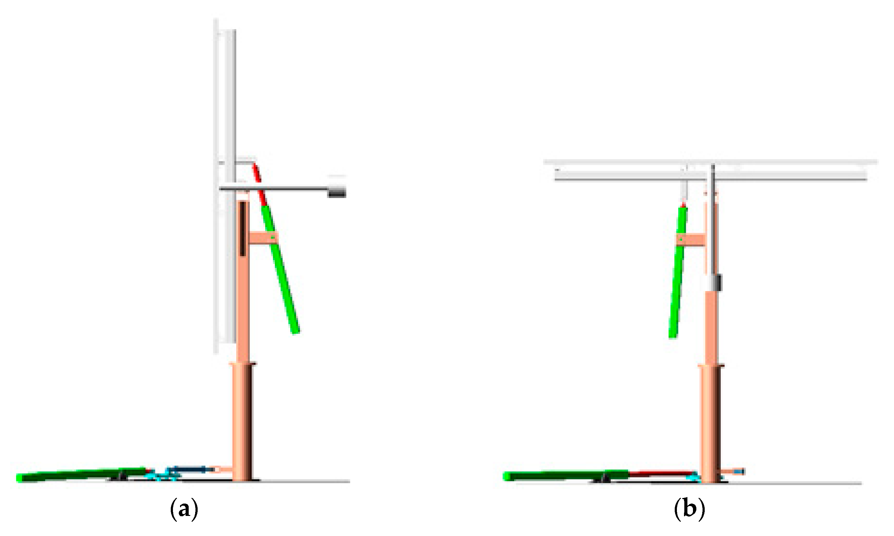
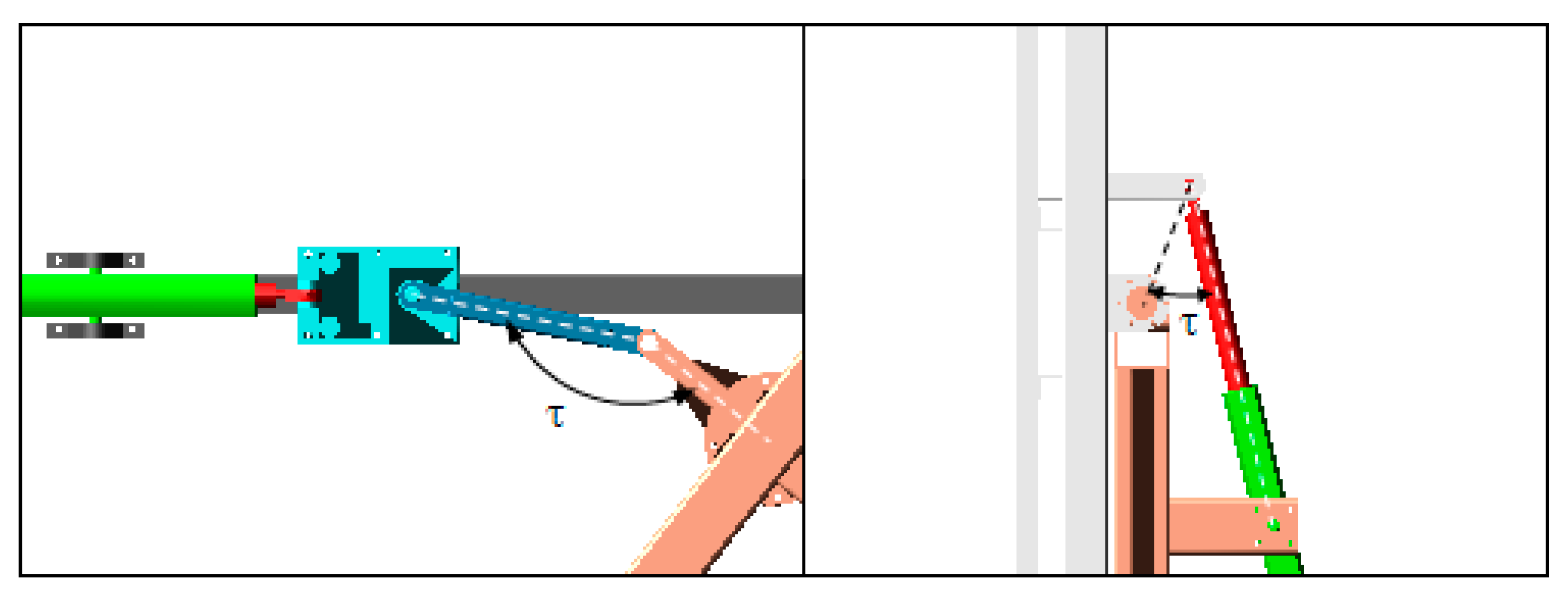
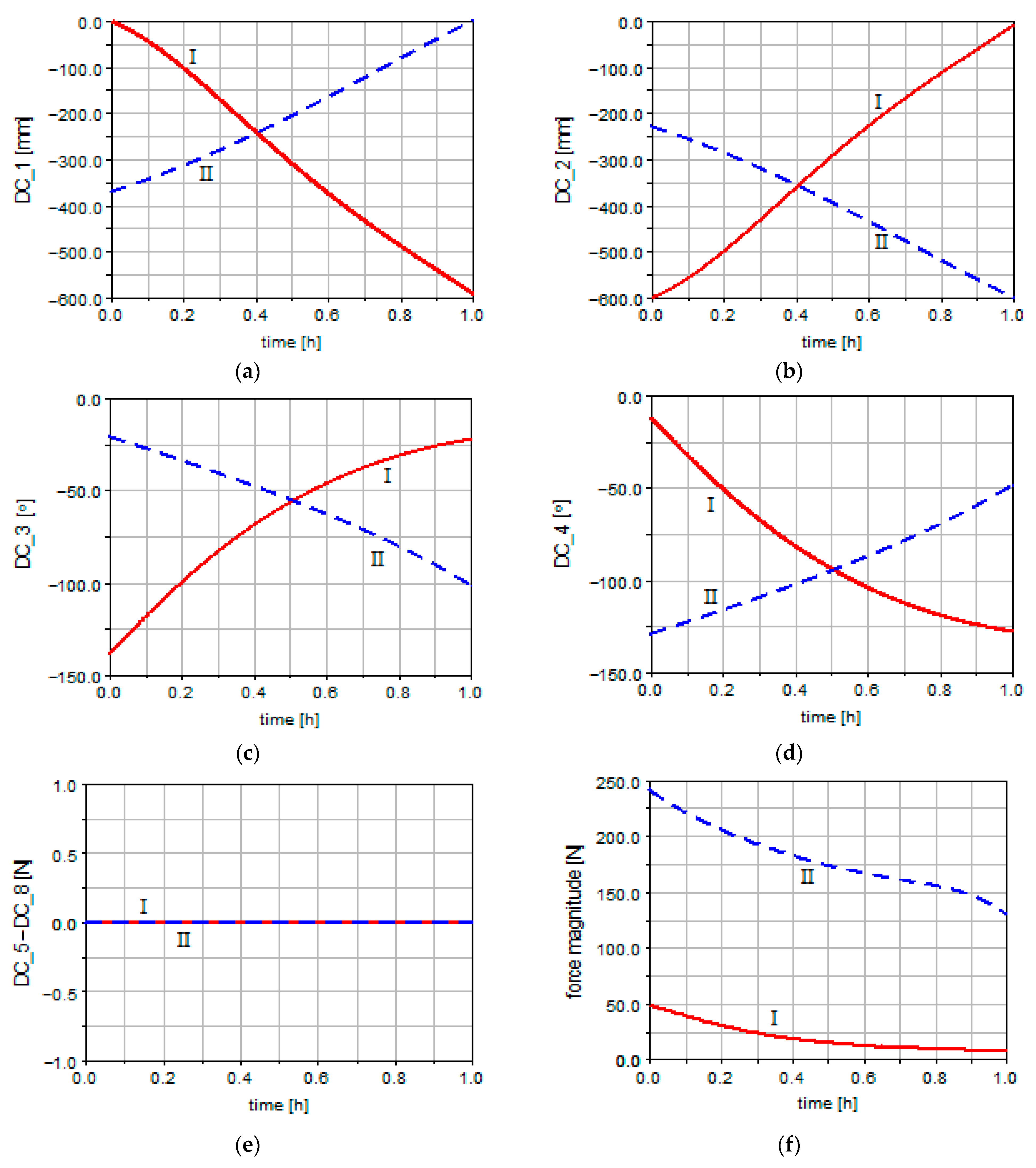
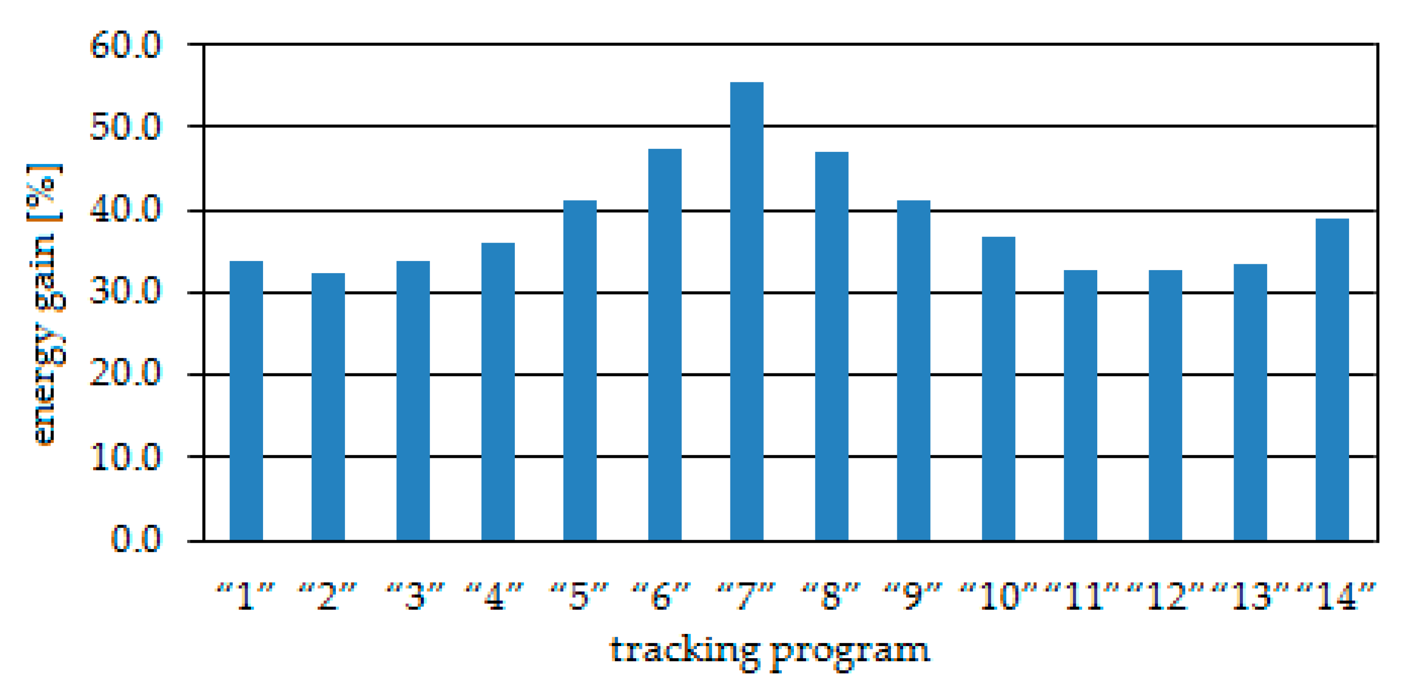
Table 1.
The energy gain brought by some PV tracking systems.
| Solar Tracker Type | Control Strategy | Location | Energy Gain | Ref. |
|---|---|---|---|---|
| bi-axial | open-loop | 45.657974 N, 25.601198 E | 41.45% | [9] |
| mono-axial | open-loop | 25.037519 N, 121.563679 E | 24.2% | [10] |
| bi-axial | closed-loop | 12.824342 N, 101.216274 E | 44.89% | [11] |
| mono-axial/bi-axial | closed-loop | 13.072090 N, 80.201859 E | 20%/40% | [12] |
| mono-axial/bi-axial | open-loop | 45.957481 N, 15.494230 E | 30.04%/39.96% | [13] |
| bi-axial | open-loop | 3.023284 N, 101.715903 E | 26.9% | [14] |
Table 2.
Tracking program “1”/“13”.
| Movement | Diurnal | Elevation | |||
|---|---|---|---|---|---|
| Angular Range | ψ* ∊ [57, −57]° | α* ∊ [11, 30]° | |||
| Actuation Time|Step Size | t [h] | Δψ* [°] | t [h] | Δα* [°] | |
| Tracking step number | 1 | 9.12 | 18 | 9.77 | 19 |
| 2 | 10.45 | 18 | 14.77 | −19 | |
| 3 | 11.68 | 21 | |||
| 4 | 12.85 | 21 | |||
| 5 | 14.10 | 18 | |||
| 6 | 15.42 | 18 | |||
| 7 | 21.30 | −114 | |||
Table 3.
Tracking program “2”/“12”.
| Movement | Diurnal | Elevation | |||
|---|---|---|---|---|---|
| Angular Range | ψ* ∊ [67, −67]° | α* ∊ [10, 38]° | |||
| Actuation Time|Step Size | t [h] | Δψ* [°] | t [h] | Δα* [°] | |
| Tracking step number | 1 | 8.85 | 21 | 8.58 | 17 |
| 2 | 10.35 | 22 | 10.58 | 11 | |
| 3 | 11.67 | 24 | 13.98 | −11 | |
| 4 | 12.92 | 24 | 15.98 | −17 | |
| 5 | 14.23 | 22 | |||
| 6 | 15.73 | 21 | |||
| 7 | 21.30 | −134 | |||
Table 4.
Tracking program “3”/“11”.
| Movement | Diurnal | Elevation | |||
|---|---|---|---|---|---|
| Angular Range | ψ* ∊ [76, −76]° | α* ∊ [15, 44]° | |||
| Actuation Time|Step Size | t [h] | Δψ* [°] | t [h] | Δα* [°] | |
| Tracking step number | 1 | 8.60 | 23 | 8.30 | 13 |
| 2 | 10.27 | 25 | 10.05 | 16 | |
| 3 | 11.67 | 28 | 14.55 | −16 | |
| 4 | 12.93 | 28 | 16.30 | −13 | |
| 5 | 14.33 | 25 | |||
| 6 | 16.00 | 23 | |||
| 7 | 21.30 | −152 | |||
Table 5.
Tracking program “4”/“10”.
| Movement | Diurnal | Elevation | |||
|---|---|---|---|---|---|
| Angular Range | ψ* ∊ [86, −86]° | α* ∊ [10, 50]° | |||
| Actuation Time|Step Size | t [h] | Δψ* [°] | t [h] | Δα* [°] | |
| Tracking step number | 1 | 7.90 | 18 | 7.80 | 20 |
| 2 | 9.27 | 17 | 9.80 | 20 | |
| 3 | 10.50 | 23 | 14.80 | −20 | |
| 4 | 11.73 | 28 | 16.78 | −20 | |
| 5 | 12.88 | 28 | |||
| 6 | 14.10 | 23 | |||
| 7 | 15.35 | 17 | |||
| 8 | 16.72 | 18 | |||
| 9 | 21.30 | −172 | |||
Table 6.
Tracking program “5”/“9”.
| Movement | Diurnal | Elevation | |||
|---|---|---|---|---|---|
| Angular Range | ψ* ∊ [90, −90]° | α* ∊ [12, 56]° | |||
| Actuation Time|Step Size | t [h] | Δψ* [°] | t [h] | Δα* [°] | |
| Tracking step number | 1 | 7.82 | 15 | 7.82 | 22 |
| 2 | 9.03 | 15 | 9.82 | 22 | |
| 3 | 10.08 | 18 | 14.82 | −22 | |
| 4 | 11.08 | 21 | 16.82 | −22 | |
| 5 | 11.93 | 21 | |||
| 6 | 12.68 | 21 | |||
| 7 | 13.53 | 21 | |||
| 8 | 14.53 | 18 | |||
| 9 | 15.58 | 15 | |||
| 10 | 16.80 | 15 | |||
| 11 | 21.30 | −180 | |||
Table 7.
Tracking programs “6”/“8”.
| Movement | Diurnal | Elevation | |||
|---|---|---|---|---|---|
| Angular Range | ψ* ∊ [90, −90]° | α* ∊ [10, 62]° | |||
| Actuation Time|Step Size | t [h] | Δψ* [°] | t [h] | Δα* [°] | |
| Tracking step number | 1 | 8.08 | 12 | 6.92 | 20 |
| 2 | 9.12 | 13 | 8.82 | 16 | |
| 3 | 10.08 | 17 | 10.32 | 16 | |
| 4 | 11.07 | 24 | 14.32 | −16 | |
| 5 | 11.93 | 24 | 15.82 | −16 | |
| 6 | 12.68 | 24 | 17.72 | −20 | |
| 7 | 13.57 | 24 | |||
| 8 | 14.53 | 17 | |||
| 9 | 15.52 | 13 | |||
| 10 | 16.53 | 12 | |||
| 11 | 21.30 | −180 | |||
Table 8.
Tracking program “7”.
| Movement | Diurnal | Elevation | |||
|---|---|---|---|---|---|
| Angular Range | ψ* ∊ [90, −90]° | α* ∊ [10, 67]° | |||
| Actuation Time|Step Size | t [h] | Δψ* [°] | t [h] | Δα* [°] | |
| Tracking step number | 1 | 8.23 | 9 | 6.70 | 20 |
| 2 | 9.08 | 12 | 8.60 | 18 | |
| 3 | 10.00 | 16 | 10.30 | 19 | |
| 4 | 11.02 | 26 | 14.30 | −19 | |
| 5 | 11.92 | 27 | 16.00 | −18 | |
| 6 | 12.68 | 27 | 17.90 | −20 | |
| 7 | 13.58 | 26 | |||
| 8 | 14.60 | 16 | |||
| 9 | 15.52 | 12 | |||
| 10 | 16.37 | 9 | |||
| 11 | 21.30 | −180 | |||
Table 9.
Tracking program “14”.
| Movement | Diurnal | Elevation | |||
|---|---|---|---|---|---|
| Angular Range | ψ* ∈ [50, −50]° | α* ∈ [10, 23]° | |||
| Actuation Time|Step Size | t [h] | Δψ* [°] | t [h] | Δα* [°] | |
| Tracking step number | 1 | 9.12 | 17 | 9.77 | 13 |
| 2 | 10.45 | 16 | 14.77 | −13 | |
| 3 | 11.68 | 17 | |||
| 4 | 12.85 | 17 | |||
| 5 | 14.10 | 16 | |||
| 6 | 15.42 | 17 | |||
| 7 | 21.30 | −100 | |||
Table 10.
The efficiency of the bi-axial solar tracker.
| Tracking Program | ET [Wh/day] | EF [Wh/day] | EC [Wh/day] | ξ [%] | ETmax [Wh/day] | εT [%] | ||
|---|---|---|---|---|---|---|---|---|
| Diurnal | Elevation | Total | ||||||
| “1” | 10,102.05 | 7520.97 | 14.18 | 27.40 | 41.58 | 33.77 | 10,201.77 | 99.02 |
| “2” | 11,943.88 | 8989.66 | 17.58 | 40.78 | 58.36 | 32.21 | 12,039.82 | 99.20 |
| “3” | 13,863.88 | 10,305.65 | 20.82 | 42.87 | 63.69 | 33.91 | 13,978.59 | 99.18 |
| “4” | 14,668.57 | 10,716.33 | 24.50 | 58.96 | 83.46 | 36.10 | 14,780.23 | 99.24 |
| “5” | 16,006.77 | 11,282.97 | 26.21 | 65.29 | 91.50 | 41.06 | 16,130.91 | 99.23 |
| “6” | 16,964.13 | 11,438.8 | 26.22 | 77.16 | 103.38 | 47.40 | 17,101.23 | 99.20 |
| “7” | 17,932.92 | 11,470.24 | 26.23 | 84.62 | 110.85 | 55.38 | 18,175.76 | 98.66 |
| “8” | 16,838.91 | 11,375.38 | 26.22 | 77.16 | 103.38 | 47.12 | 16,974.03 | 99.20 |
| “9” | 15,880.73 | 11,190.47 | 26.21 | 65.29 | 91.50 | 41.10 | 16,005.34 | 99.22 |
| “10” | 14,790.47 | 10,768.21 | 24.50 | 58.96 | 83.46 | 36.58 | 14,904.31 | 99.24 |
| “11” | 12,800.96 | 9610.99 | 20.82 | 42.88 | 63.70 | 32.53 | 12,926.05 | 99.03 |
| “12” | 11,982.89 | 8990.86 | 17.58 | 40.78 | 58.36 | 32.63 | 12,083.36 | 99.17 |
| “13” | 9692.3 | 7223.07 | 14.18 | 27.40 | 41.58 | 33.61 | 9779.61 | 99.11 |
| “14” | 7384.46 | 5289.51 | 11.97 | 18.49 | 30.46 | 39.03 | 7429.62 | 99.39 |
Publisher’s Note: MDPI stays neutral with regard to jurisdictional claims in published maps and institutional affiliations. |
© 2021 by the author. Licensee MDPI, Basel, Switzerland. This article is an open access article distributed under the terms and conditions of the Creative Commons Attribution (CC BY) license (http://creativecommons.org/licenses/by/4.0/).
Share and Cite
MDPI and ACS Style
Alexandru, C. Optimization of the Bi-Axial Tracking System for a Photovoltaic Platform. Energies 2021, 14, 535. https://doi.org/10.3390/en14030535
AMA Style
Alexandru C. Optimization of the Bi-Axial Tracking System for a Photovoltaic Platform. Energies. 2021; 14(3):535. https://doi.org/10.3390/en14030535
Chicago/Turabian StyleAlexandru, Cătălin. 2021. "Optimization of the Bi-Axial Tracking System for a Photovoltaic Platform" Energies 14, no. 3: 535. https://doi.org/10.3390/en14030535
Note that from the first issue of 2016, this journal uses article numbers instead of page numbers. See further details here.