Analysis of Induced Voltage on Pipeline Located Close to Parallel Distribution System

Abstract

Gas and oil pipelines are widely used to supply customers. They are often laid in parallel with high voltage power lines, sharing right of way. When the pipeline is located near overhead high-voltage power, corrosion caused by induced voltages from AC power lines can occur in utility pipelines. Therefore, the calculation of induced voltage is always required for both interference and maintenance workers as well as pipeline facility safety. For parallel distribution lines, the calculation method for the induced voltage is not suitable due to the excessive error caused by using the screening factors of the neutral current. For a more practical analysis of the induced voltage, a new analysis is needed using the actual neutral current and which also considers the overhead ground conductor and the neutral conductor. This paper analyzed the induced voltage from a parallel distribution system using Carson’s formula and vector analysis. Simulation analysis results are verified by separate Electromagnetic Transient Program (EMTP) simulation.

1. Introduction

There are important issues to consider by both electrical utilities and pipeline operators when an underground pipeline is located proximal to the ground level in overhead high-voltage power lines [1,2,3,4,5,6], namely safety and corrosion. Due to the corrosion of gas and oil pipelines caused by induced voltages from AC power lines [2,3,4,5], a pipeline AC mitigation system is needed to avoid costly repairs and maintenance. The primary focus of mitigation is to reduce the induced voltages at normal and fault conditions according to the NACE standard [6] for the safety of maintenance operators and damage in pipeline facilities. This corrosion can also lead to an equipment malfunction [7,8].

The interferences through which the AC power lines generate induced voltage and current on nearby pipes are inductive coupling and conductive coupling. The inductive coupling is related to the electromotive force (EMF) induced in the pipe–earth circuit, while the conductive coupling is caused by the injection of current into the soil by a transmission line during phase-to-ground fault conditions or subjected to currents [9].

The interference issue of induced voltage on pipelines parallel to power lines has been treated a lot in the literature [10,11,12]. Recent literature related to this issue was published by A. Popoli [13], who analyzed interference caused by the vicinity of a metallic pipeline buried in the soil to a transmission line using parameters calculated with the finite difference method (FEM). G. Lucca [9] analyzed the induced voltage and current from a transmission line in fault condition on a nearby buried pipeline with the EMF. However, these works focus on the interference of transmission lines and pipelines.

There are many reports on the electromagnetic interference (EM) of the induced voltage using the Electromagnetic Transient Program (EMTP) [14,15,16,17]. A practical calculation method using EMTP is presented in [14], which assumes multi-conductor power lines with a variety of tower types (complex approximation layouts), and multilayered soil models are parallel to a nearby pipeline. Heo et al. [15] analyzed the induced voltage generated by overhead transmission lines under normal cases using the line and cable constant (LCC) module. Isogai and Ametani [16] analyzed the effect of induced voltages to the pipeline on power lines. The results show the three-phase horizontal lines tend to induce higher voltages than vertical lines when the same system parameters for the transmission line and ground are used.

In order to reduce the electromagnetic interference between power lines and pipelines, the most practical solution consists in worsening the electromagnetic coupling. Then, “the use of screening conductors buried in the soil above the metallic pipelines appears as a feasible solution to attenuate the voltage generated on the pipeline” by power lines [18]. Especially for designing an optimized mitigation system, a proper calculation is required to accurately predict the induced voltage on metallic pipelines.

Previous research on induced voltage is mainly focused on overhead transmission lines [8,9,10,11,12,13,14,15,16]. The induced voltage on the pipeline is critical because the unbalanced current flow in the distribution system can increase the induced voltage on the pipeline. Recently, it has been relatively common to find double-circuit lines (DCL) where distribution lines are physically parallel due to their significant environmental and economic advantages over single-circuit lines (SCL). Thus, it is necessary to analyze induced voltage from DCL [19,20,21].

The calculation method in [22] is not suitable for parallel distribution lines due to the excessive error caused by using a constant screening factor of the neutral current. The constant value of the screening factors that are currently used in the calculation of the induced voltage in distribution lines is the main cause of error [23,24], as it cannot consider unbalanced loading conditions in the distribution line. Thus, a new practical method is needed for analyzing the induced voltage using the actual neutral current without using the screening factors from the overhead ground conductor and the neutral conductor.

Two types of overhead distribution lines, SCL and DCL, are considered in this paper. These two types of distribution line circuits are only available from the Korea Electric Power Corporation (KEPCO) in Korea. The modeling and calculation methods of induced voltages using the actual neutral current from SCL and DCL distribution line models are presented in Section 2. The simulation results, vector analysis based on the simulation results, and comparison of case studies are demonstrated in Section 3. The conclusions are presented in Section 4.

2. Voltage Calculation between Pipeline and Distribution System

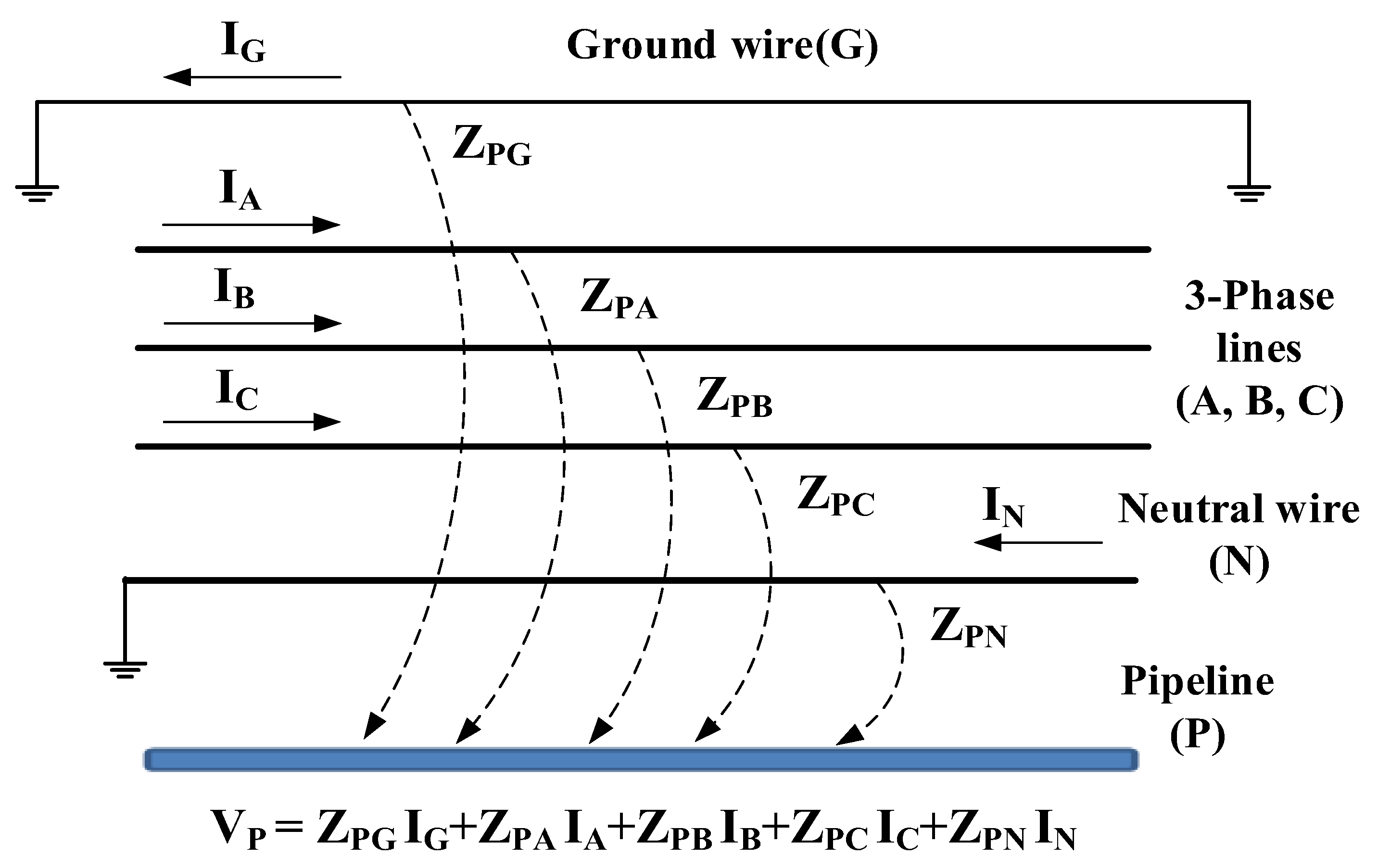
2.1. Induced Voltage Calculation in SCL

Figure 1 depicts an SCL overhead distribution laid parallel to the pipeline line. The ground wire, G indicates the overhead ground conductor. Subscripts A, B, C, N, and P indicate the conductor phase A, B, C, neutral, and pipeline, respectively.

An induced voltage on the pipeline line can be calculated using Carson’s formula [9,23]. The relationship between voltage and current from Figure 1 is defined:

$$\left[\begin{array}{c}{\mathit{V}}_{\mathit{G}}\\ {\mathit{V}}_{\mathit{A}}\\ {\mathit{V}}_{\mathit{B}}\\ {\mathit{V}}_{\mathit{C}}\\ {\mathit{V}}_{\mathit{N}}\\ {\mathit{V}}_{\mathit{P}}\end{array}\right]=\left[\begin{array}{cccccc}{\mathit{Z}}_{\mathit{GG}}& {\mathit{Z}}_{\mathit{GA}}& {\mathit{Z}}_{\mathit{GB}}& {\mathit{Z}}_{\mathit{GC}}& {\mathit{Z}}_{\mathit{GN}}& {\mathit{Z}}_{\mathit{GP}}\\ {\mathit{Z}}_{\mathit{AG}}& {\mathit{Z}}_{\mathit{AA}}& {\mathit{Z}}_{\mathit{AB}}& {\mathit{Z}}_{\mathit{AC}}& {\mathit{Z}}_{\mathit{AN}}& {\mathit{Z}}_{\mathit{AP}}\\ {\mathit{Z}}_{\mathit{BG}}& {\mathit{Z}}_{\mathit{BA}}& {\mathit{Z}}_{\mathit{BB}}& {\mathit{Z}}_{\mathit{BC}}& {\mathit{Z}}_{\mathit{BN}}& {\mathit{Z}}_{\mathit{BP}}\\ {\mathit{Z}}_{\mathit{CG}}& {\mathit{Z}}_{\mathit{CA}}& {\mathit{Z}}_{\mathit{CB}}& {\mathit{Z}}_{\mathit{CC}}& {\mathit{Z}}_{\mathit{CN}}& {\mathit{Z}}_{\mathit{CP}}\\ {\mathit{Z}}_{\mathit{NG}}& {\mathit{Z}}_{\mathit{NA}}& {\mathit{Z}}_{\mathit{NB}}& {\mathit{Z}}_{\mathit{NC}}& {\mathit{Z}}_{\mathit{NN}}& {\mathit{Z}}_{\mathit{NP}}\\ {\mathit{Z}}_{\mathit{PG}}& {\mathit{Z}}_{\mathit{PA}}& {\mathit{Z}}_{\mathit{PB}}& {\mathit{Z}}_{\mathit{PC}}& {\mathit{Z}}_{\mathit{PN}}& {\mathit{Z}}_{\mathit{PP}}\end{array}\right]\left[\begin{array}{c}{\mathit{I}}_{\mathit{G}}\\ {\mathit{I}}_{\mathit{A}}\\ {\mathit{I}}_{\mathit{B}}\\ {\mathit{I}}_{\mathit{C}}\\ {\mathit{I}}_{\mathit{N}}\\ {\mathit{I}}_{\mathit{P}}\end{array}\right]$$

(1)

where the calculation of neutral current assumes that the neutral grounding point of the 3-phase lines is common [19].

The self and mutual impedance are obtained by Carson’s formula. The mutual impedance of the system can be calculated as a lump sum of impedances between each conductor and the pipeline [23,25].

$$\begin{array}{l}{\mathit{Z}}_{\mathit{i}\mathit{i}}=\mathit{R}+1.588{\mathit{e}}^{-3}\mathit{f}+2.022{\mathit{e}}^{-3}\mathit{f}\left(\ln \frac{1}{\mathit{G}\mathit{M}\mathit{R}}+7.6786+\frac{1}{2}\ln \frac{\rho }{\mathit{f}}\right)\\ {\mathit{Z}}_{\mathit{i}\mathit{j}}=1.588{\mathit{e}}^{-3}\mathit{f}+2.022{\mathit{e}}^{-3}\mathit{f}\left(\ln \frac{1}{{\mathit{D}}_{\mathit{i}\mathit{j}}}+7.6786+\frac{1}{2}\ln \frac{\rho }{\mathit{f}}\right)\end{array}$$

(2)

where

• R = resistance of the conductor;
• GMR = geometric mean radius of the conductor;
• Ρ = earth resistivity;
• f = system frequency;
• D_ij = distance from conductor i to conductor j;
• Z_ii = self-impedance of the conductor I;
• Z_ij = mutual impedance between conductors i and j.

The voltage of the overhead ground conductor (V_G) is expressed:

$${\mathit{V}}_{\mathit{G}}={\mathit{Z}}_{\mathit{GG}}{\mathit{I}}_{\mathit{G}}+{\mathit{Z}}_{\mathit{GA}}{\mathit{I}}_{\mathit{A}}+{\mathit{Z}}_{\mathit{GB}}{\mathit{I}}_{\mathit{B}}+{\mathit{Z}}_{\mathit{GC}}{\mathit{I}}_{\mathit{C}}+{\mathit{Z}}_{\mathit{GN}}{\mathit{I}}_{\mathit{N}}={\mathit{Z}}_{\mathit{GG}}{\mathit{I}}_{\mathit{G}}+{\mathit{Z}}_{\mathit{GABC}}{\mathit{I}}_{\mathit{ABC}}+{\mathit{Z}}_{\mathit{GN}}{\mathit{I}}_{\mathit{N}}$$

(3)

where

$$\begin{array}{l}{\mathit{Z}}_{\mathit{GABC}}{\mathit{I}}_{\mathit{ABC}}={\mathit{Z}}_{\mathit{GA}}{\mathit{I}}_{\mathit{A}}+{\mathit{Z}}_{\mathit{GB}}{\mathit{I}}_{\mathit{B}}+{\mathit{Z}}_{\mathit{GA}}{\mathit{I}}_{\mathit{C}}\\ {\mathit{I}}_{\mathit{N}}={\mathit{I}}_{\mathit{A}}+{\mathit{I}}_{\mathit{B}}+{\mathit{I}}_{\mathit{C}}\end{array}$$

Overhead ground conductors are on top of the distribution lines to avoid lightning strikes. V_G can be assumed to be zero [15] because it is grounded. Accordingly, the current of the overhead ground conductor, I_G can be obtained on the

$${\mathit{I}}_{\mathit{G}}=-\frac{{\mathit{Z}}_{\mathit{GABC}}{\mathit{I}}_{\mathit{ABC}}+{\mathit{Z}}_{\mathit{GN}}{\mathit{I}}_{\mathit{N}}}{{\mathit{Z}}_{\mathit{GG}}}$$

(4)

Then, the induced voltage, V_P on the pipeline, can be calculated:

$$\begin{array}{cc}\hfill {\mathit{V}}_{\mathit{P}}& ={\mathit{Z}}_{\mathit{PG}}{\mathit{I}}_{\mathit{G}}+{\mathit{Z}}_{\mathit{PA}}{\mathit{I}}_{\mathit{A}}+{\mathit{Z}}_{\mathit{PB}}{\mathit{I}}_{\mathit{B}}+{\mathit{Z}}_{\mathit{PC}}{\mathit{I}}_{\mathit{C}}+{\mathit{Z}}_{\mathit{PN}}{\mathit{I}}_{\mathit{N}}\hfill \\ & ={\mathit{Z}}_{\mathit{PG}}{\mathit{I}}_{\mathit{G}}+{\mathit{Z}}_{\mathit{PABC}}{\mathit{I}}_{\mathit{ABC}}+{\mathit{Z}}_{\mathit{PN}}{\mathit{I}}_{\mathit{N}}\hfill \\ & ={\mathit{V}}_{\mathit{G}}+{\mathit{V}}_{\mathit{ABC}}+{\mathit{V}}_{\mathit{N}}\hfill \end{array}$$

(5)

where

$${\mathit{Z}}_{\mathit{PABC}}{\mathit{I}}_{\mathit{ABC}}={\mathit{Z}}_{\mathit{PA}}{\mathit{I}}_{\mathit{A}}+{\mathit{Z}}_{\mathit{PB}}{\mathit{I}}_{\mathit{B}}+{\mathit{Z}}_{\mathit{PC}}{\mathit{I}}_{\mathit{c}}$$

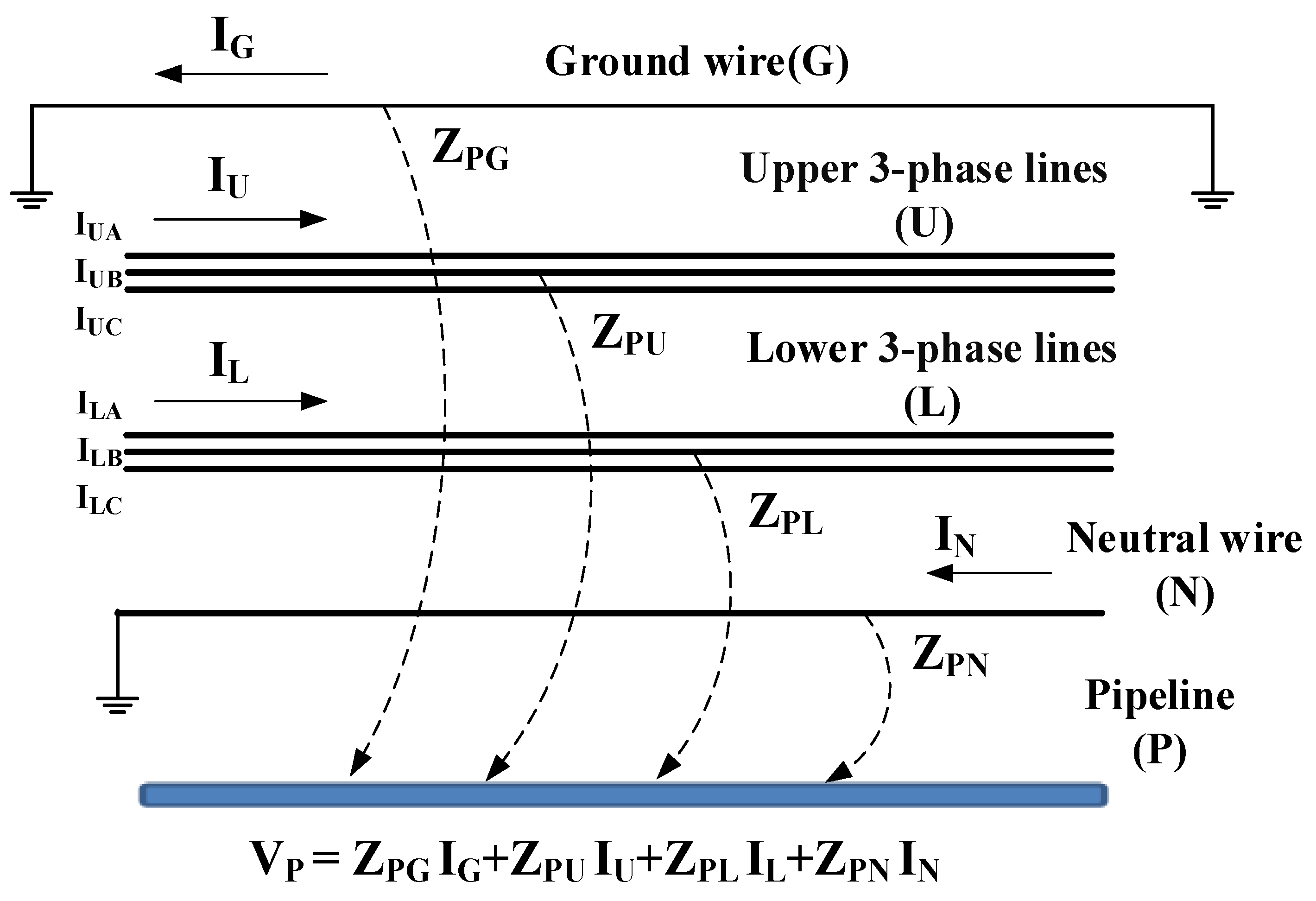
2.2. Induced Voltage Calculation in DCL

Figure 1 depicts the SCL overhead distribution laid parallel to the pipeline line. The ground wire, G, indicates the overhead ground.

Figure 2 depicts the DCL overhead distribution system laid parallel to the pipeline line. A matrix extension [23] is applied to calculate the induced voltage in the DCL. The subscripts U and L indicate the upper and lower 3-phase lines, respectively.

Then, the pipeline laid parallel to the overhead distribution line with the DCL can be expressed:

(6)

Mutual impedance matrices (Z_XY) in Equation (6) represent the parallel overhead distribution lines and the pipeline. These matrices are applied to calculate the induced voltage of the pipeline and take into account the coupling with adjacent parallel distribution lines. Thus, for example:

$$\begin{array}{cc}\hfill {\mathit{V}}_{\mathit{G}}& ={\mathit{Z}}_{\mathit{GG}}{\mathit{I}}_{\mathit{G}}+{\mathit{Z}}_{\mathit{GUA}}{\mathit{I}}_{\mathit{UA}}+{\mathit{Z}}_{\mathit{GUB}}{\mathit{I}}_{\mathit{UB}}+{\mathit{Z}}_{\mathit{GUC}}{\mathit{I}}_{\mathit{UC}}+{\mathit{Z}}_{\mathit{GLA}}{\mathit{I}}_{\mathit{LB}}+{\mathit{Z}}_{\mathit{GLB}}{\mathit{I}}_{\mathit{LB}}+{\mathit{Z}}_{\mathit{GLC}}{\mathit{I}}_{\mathit{LC}}+{\mathit{Z}}_{\mathit{GN}}{\mathit{I}}_{\mathit{N}}\hfill \\ \hfill & ={\mathit{Z}}_{\mathit{GG}}{\mathit{I}}_{\mathit{G}}+{\mathit{Z}}_{\mathit{GU}}{\mathit{I}}_{\mathit{U}}+{\mathit{Z}}_{\mathit{GL}}{\mathit{I}}_{\mathit{L}}+{\mathit{Z}}_{\mathit{GN}}{\mathit{I}}_{\mathit{N}}\hfill \end{array}$$

(7)

where

$$\begin{array}{l}{\mathit{Z}}_{\mathit{GU}}{\mathit{I}}_{\mathit{U}}={\mathit{Z}}_{\mathit{GUA}}{\mathit{I}}_{\mathit{UA}}+{\mathit{Z}}_{\mathit{GUB}}{\mathit{I}}_{\mathit{UB}}+{\mathit{Z}}_{\mathit{GUC}}{\mathit{I}}_{\mathit{UC}}\\ {\mathit{Z}}_{\mathit{GL}}{\mathit{I}}_{\mathit{L}}={\mathit{Z}}_{\mathit{GLA}}{\mathit{I}}_{\mathit{LB}}+{\mathit{Z}}_{\mathit{GLB}}{\mathit{I}}_{\mathit{LB}}+{\mathit{Z}}_{\mathit{GLC}}{\mathit{I}}_{\mathit{LC}}\end{array}$$

V_G can be assumed to be zero in the DCL configuration [21], so the current of the overhead ground conductor can be determined:

$${\mathit{I}}_{\mathit{G}}=-\frac{{\mathit{Z}}_{\mathit{GU}}{\mathit{I}}_{\mathit{U}}+{\mathit{Z}}_{\mathit{GL}}{\mathit{I}}_{\mathit{L}}+{\mathit{Z}}_{\mathit{GN}}{\mathit{I}}_{\mathit{N}}}{{\mathit{Z}}_{\mathit{GG}}}$$

(8)

For DCLs, we assume the upper and lower side use the common ground of the neutral line, which is equal to the total current of the upper and lower sides using the superposition method [19]. Then, the neutral current can be calculated:

$${\mathit{I}}_{\mathit{N}}={\mathit{I}}_{\mathit{UA}}+{\mathit{I}}_{\mathit{UB}}+{\mathit{I}}_{\mathit{UC}}+{\mathit{I}}_{\mathit{LA}}+{\mathit{I}}_{\mathit{LB}}+{\mathit{I}}_{\mathit{LC}}$$

(9)

Then, the pipeline-induced voltage (V_P) in the DCL can be calculated using this result:

$$\begin{array}{cc}\hfill {\mathit{V}}_{\mathit{P}}& ={\mathit{Z}}_{\mathit{PG}}{\mathit{I}}_{\mathit{G}}+{\mathit{Z}}_{\mathit{PU}}{\mathit{I}}_{\mathit{U}}+{\mathit{Z}}_{\mathit{PL}}{\mathit{I}}_{\mathit{L}}+{\mathit{Z}}_{\mathit{PN}}{\mathit{I}}_{\mathit{N}}\hfill \\ \hfill & ={\mathit{V}}_{\mathit{G}}+{\mathit{V}}_{\mathit{U}}+{\mathit{V}}_{\mathit{L}}+{\mathit{V}}_{\mathit{N}}\hfill \end{array}$$

(10)

where

$$\begin{array}{cc}\hfill & {\mathit{Z}}_{\mathit{PU}}{\mathit{I}}_{\mathit{U}}={\mathit{Z}}_{\mathit{PUA}}{\mathit{I}}_{\mathit{UA}}+{\mathit{Z}}_{\mathit{PUB}}{\mathit{I}}_{\mathit{UB}}+{\mathit{Z}}_{\mathit{PUC}}{\mathit{I}}_{\mathit{UC}}\hfill \\ \hfill & {\mathit{Z}}_{\mathit{PL}}{\mathit{I}}_{\mathit{L}}={\mathit{Z}}_{\mathit{PLA}}{\mathit{I}}_{\mathit{LA}}+{\mathit{Z}}_{\mathit{PLB}}{\mathit{I}}_{\mathit{LB}}+{\mathit{Z}}_{\mathit{PLC}}{\mathit{I}}_{\mathit{LC}}\hfill \end{array}$$

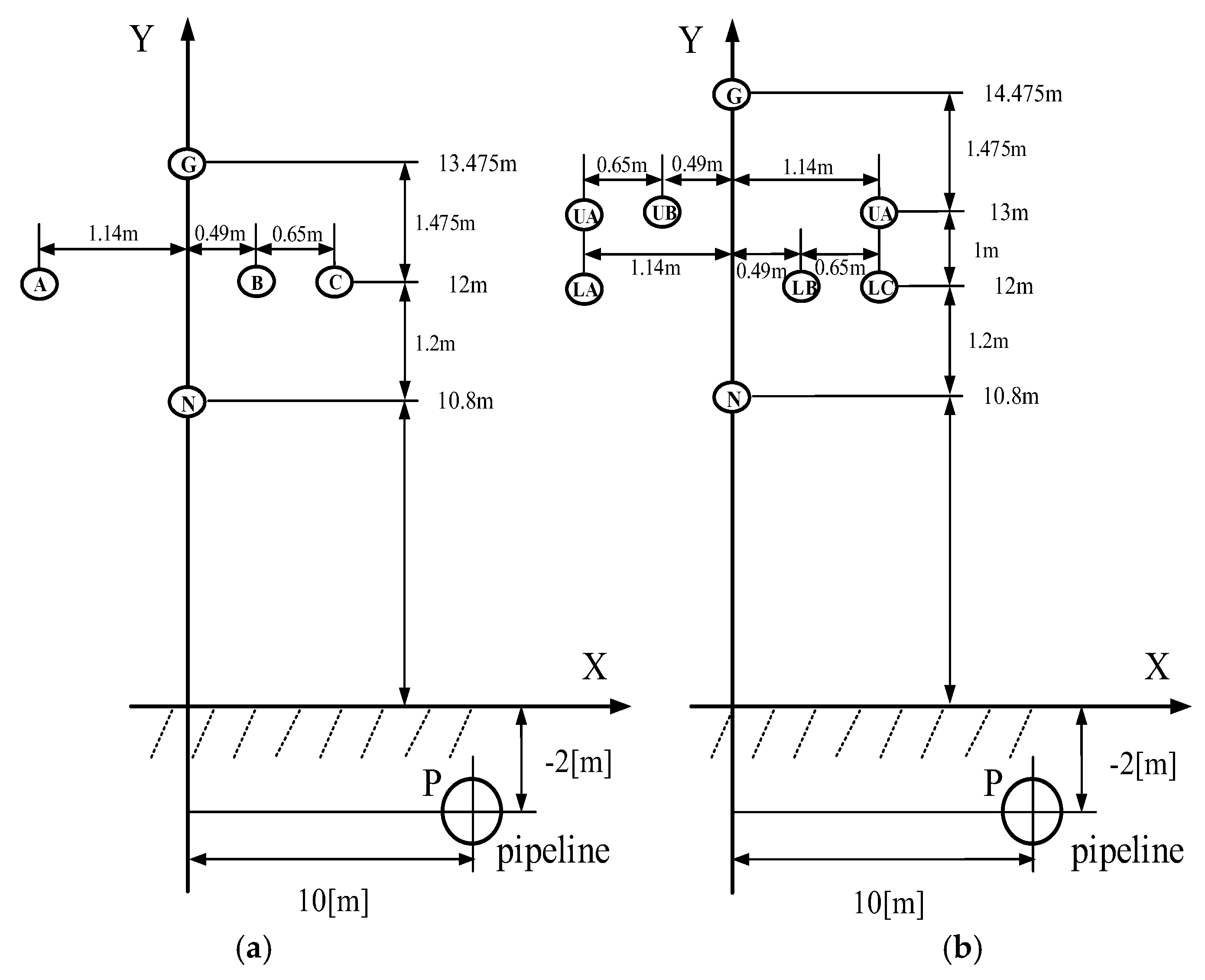
2.3. System Modeling

Figure 3 illustrates the two types of overhead distribution line (ODL) configurations with the pipeline. In this paper, to analyze the induced voltage on a pipeline located close to overhead distribution lines, the ODL is implemented in both SCL and DCL configurations, as shown in Figure 3.

Both SCL and DCL types are classified by existing distribution line types of the Korea Electric Power Corporation (KEPCO) [19]. The data obtained from the pipelines and conductors are applied in this study. The key details are listed in

Table 1. Conductor type and data.

Line Type	Cable Type (mm2)	Radius (cm)	Resistance (Ω/km)
Overhead ground conductor	ACSR 32	0.39	0.898
Distribution lines	ACSR 160	0.91	0.182
Neutral conductor	ACSR 95	0.675	0.301

and shown in Figure 4 [26].

All case studies are analyzed based on a 1 km distance of the parallel distribution lines. The system frequency, soil resistivity, and power factors are 60 (Hz), 100 (Ω m), and 0.9 (pu), respectively.

3. Simulation and Results

The induced voltage on the pipeline is analyzed using EMTP based on various conditions: unbalanced loading conditions, different pole types, and the separation distance between the ODL and the pipeline. In the case studies, V_P is a calculation value from (5), (10), V_EMTP is the EMTP simulation result, and the difference will be calculated based on V_EMTP. The unbalanced loading ratio between phases is kept to be less than 30% in the distribution.

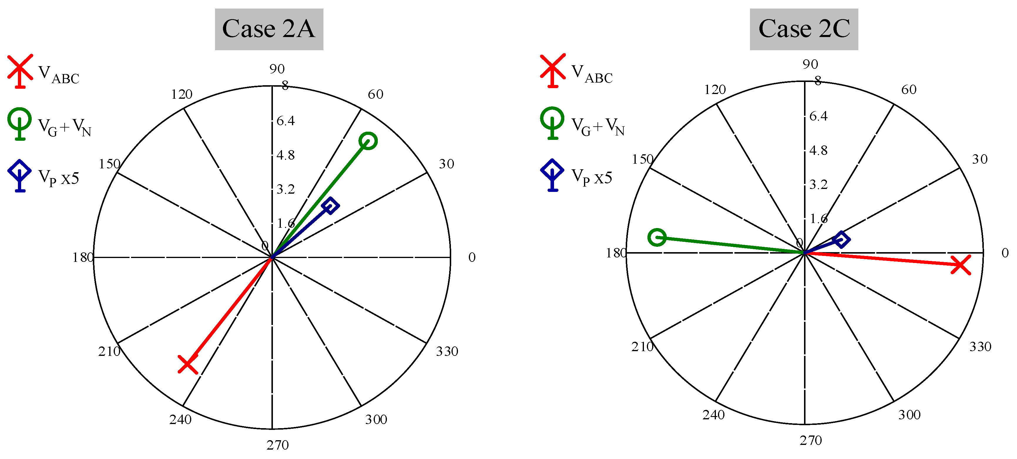
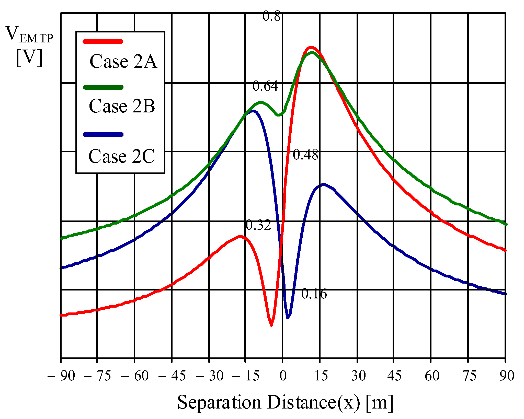
3.1. Simulation Results in SCL

The EMTP simulation result of SCL cases is shown in

Table 2. Load condition results of SCL.

Case Study	Load Condition			VP (V)	VEMTP (V)	VDiff. (%)
	A (MVA)	B (MVA)	C (MVA)
Case 1	1	1	1	0.513	0.515	0.2
Case 2A	1.3	1	1	0.713	0.716	0.3
Case 2B	1	1.3	1	0.700	0.698	0.2
Case 2C	1	1	1.3	0.353	0.356	0.3
Case 3	1	1.1	1.2	0.465	0.467	0.2

. For the SCL case study shown in Table 2, Case 1 has a balanced load, Cases 2A–2C have unbalanced single-phase loads, and Case 3 has an unbalanced three-phase load.

Table 2 shows that the difference between the calculated value and the simulation result is less than 0.3% error. The maximum and minimum induced voltage to the pipeline are found in Case 2A and Case 2C, respectively. The induced voltage in Case 2C is nearly 50% of the induced voltage from Case 2A. The simulation results indicate that the induced voltages are dependent on the load condition, as shown in Figure 3a.

By using Equation (5), the induced voltage of V_G, V_ABC, and V_N are calculated and shown in

Table 3. SCL calculation of induced voltage using (5).

Case Study	VG (V)	VABC (V)	VN (V)
Case 1	0.228 ∠ −21.60°	0.389 ∠ 48.60°	8.6 × 10−15 ∠ 163.42°
Case 2A	0.199 ∠ 14.32°	6.236 ∠ −127.33°	6.783 ∠ 52.70°
Case 2B	0.430 ∠ −21.67°	6.894 ∠ 109.67°	6.783 ∠ −67.30°
Case 2C	0.198 ∠ −57.54°	6.976 ∠ −4.71°	6.783 ∠ 172.7°
Case 3	0.262 ∠ −38.85°	4.255 ∠ 24.80°	3.919 ∠ −157.27°

. Due to the difference in direction between the V_ABC and V_G + V_N phase angles, V_ABC is defined as inducing side voltage caused by a three-phase current, and V_G + V_N is defined as a shielding side voltage caused by the current of an overhead ground conductor and a neutral conductor.

The SCL induced voltages in Table 3 are classified as shielding side, inducing side, and induced voltages, as shown in

Table 4. Inducing and shielding side analysis of SCL.

Case Study	Inducing Side	Shielding Side	Induced Voltage
	VABC (V)	VG + VN (V)	VP (V)
Case 1	0.389 ∠ 48.60°	0.228 ∠ −21.60°	0.513 ∠ 23.83°
Case 2A	6.236 ∠ −127.33°	6.940 ∠ 51.68°	0.713 ∠ 42.99°
Case 2B	6.894 ∠ 109.67°	7.090 ∠ −64.82°	0.700 ∠ 6.17°
Case 2C	6.976 ∠ −4.7°	6.658 ∠ 174.01°	0.353 ∠ 20.23°
Case 3	4.255 ∠ 24.80°	3.801 ∠ −153.79°	0.465 ∠ 13.21°

.

For single-phase unbalanced load cases, the induced voltage of Case 2C is nearly half of the induced voltage in Case 2A and 2B. This difference is due to the phase angle of the neutral current, which is closely arranged to the C-phase line and the pipeline. The shielding effect of the neutral current was verified by both calculation and vector analysis, as shown in Figure 5, where the shielding effect is multiplied by five for illustration purposes. The resultant vector V_P, V_P is much smaller than V_ABC and V_G + V_N in both Case 2A and Case 2C.

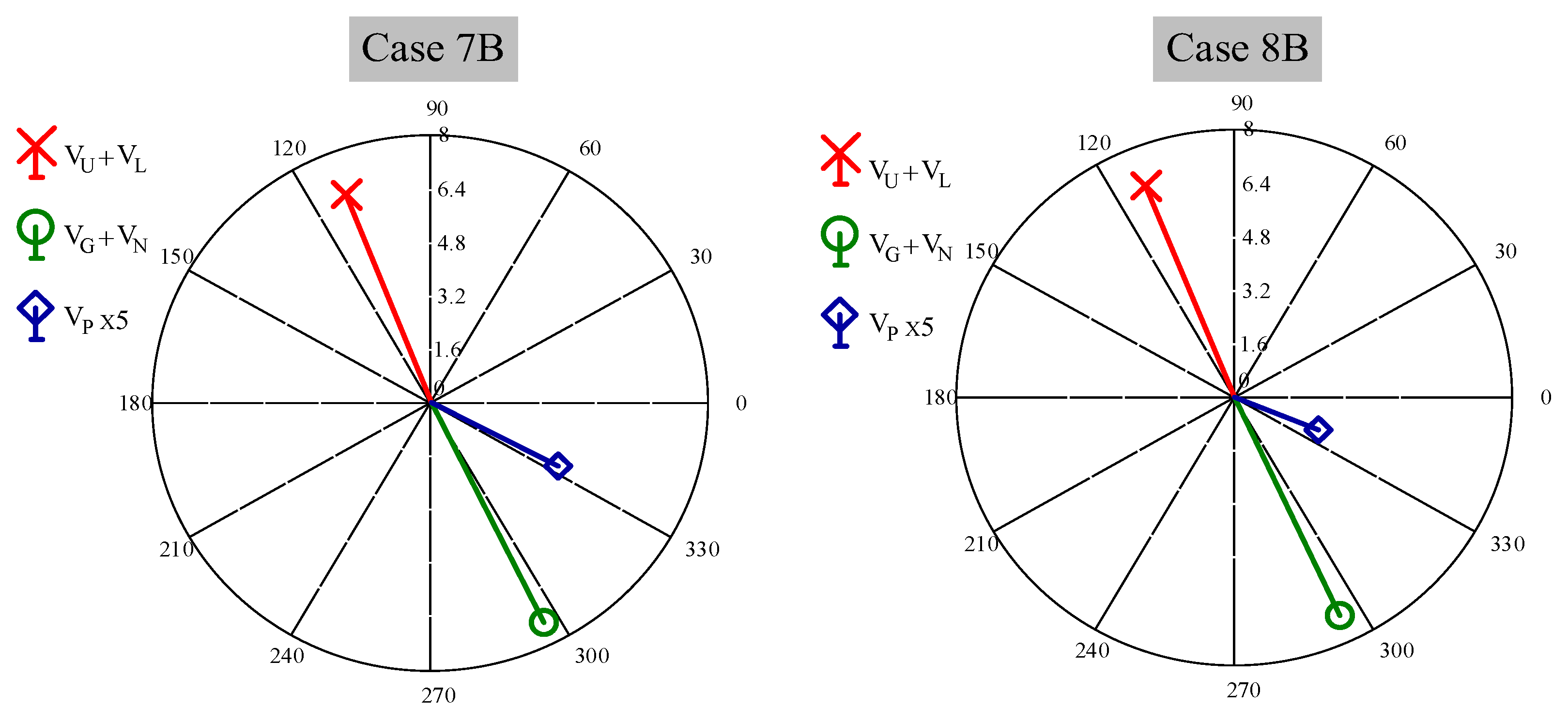
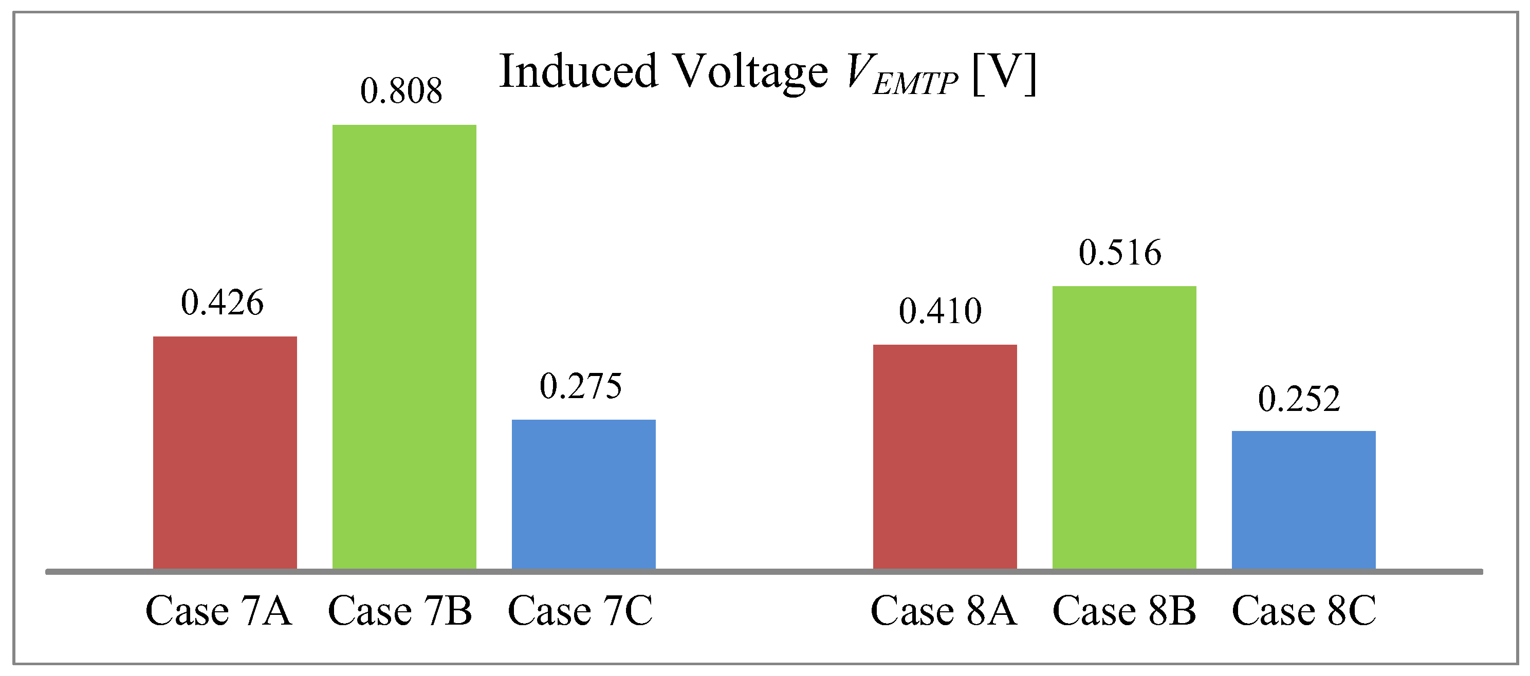
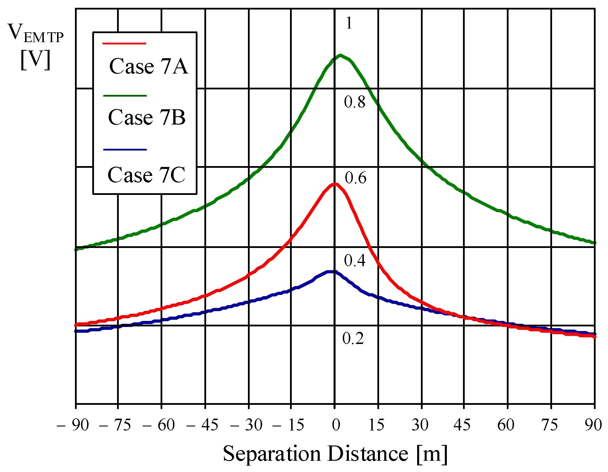
3.2. Simulation Results in DCL

For the case study of DCL, three-phase lines added from the existing SCL to the DCL were divided into the upper and the lower side, as shown in Figure 3b. The load conditions of the upper and lower sides were changed and are defined:

• Case 4: Three-phase balanced load in the upper and lower sides.
• Case 5: Single-phase (Uc, Lc-phase) unbalanced load in the upper and lower sides.
• Case 6: Three-phase unbalanced load in the upper and lower sides.
• Case 7A–7C: Single-phase unbalanced load on the upper side and balanced load on the lower side.
• Case 8A–8C: Balanced load on the upper side and single-phase unbalanced load on the lower side.

The results for V_P, which is the calculated induced voltage using Equation (10) and EMTP simulation, are compared in

Table 5. Load condition results of DCL.

Case Study	Load Condition						VP (V)	VEMTP (V)	VDiff. (%)
	UA (MVA)	UB (MVA)	UC (MVA)	LA (MVA)	LB (MVA)	LC (MVA)
Case 4	1	1	1	1	1	1	0.330	0.329	0.1
Case 5	1	1	1.3	1	1	1.3	0.401	0.388	1.3
Case 6	1	1.1	1.2	1	1.1	1.2	0.406	0.396	1.0
Case 7A	1.3	1	1	1	1	1	0.430	0.426	0.4
Case 7B	1	1.3	1	1	1	1	0.819	0.808	1.1
Case 7C	1	1	1.3	1	1	1	0.284	0.275	0.9
Case 8A	1	1	1	1.3	1	1	0.412	0.410	0.2
Case 8B	1	1	1	1	1.3	1	0.525	0.516	0.9
Case 8C	1	1	1	1	1	1.3	0.253	0.252	0.1

. The simulation results show the minimal differences between the calculated values and simulation results.

In

Table 6. DCL calculation of induced voltage using (10).

Case Study	VG (V)	VU (V)	VL (V)	VN (V)
Case 4	0.322 ∠ −21.9°	0.354 ∠ −132.7°	0.391 ∠ 48.4°	8.6 × 10−15 ∠ 172.4°
Case 5	0.343 ∠ −88.0°	6.421 ∠ −10.6°	7.041 ∠ −5°	13.697 ∠ 172.4°
Case 6	0.411 ∠ −52.6°	3.500 ∠ 19.8°	4.292 ∠ 24.5°	7.909 ∠ −157.5°
Case 7A	0.294 ∠ 26.2°	7.085 ∠ −128.0°	0.391 ∠ 48.4°	6.849 ∠ 52.4°
Case 7B	0.642 ∠ −22.0°	6.507 ∠ 114.9°	0.391 ∠ 48.4°	6.849 ∠ −67.6°
Case 7C	0.292 ∠ −70.0°	6.421 ∠ −10.6°	0.391 ∠ 48.4°	6.849 ∠ 172.4°
Case 8A	0.284 ∠ −2.0°	0.354 ∠ −132.7°	6.298 ∠ −127.6°	6.849 ∠ 52.4°
Case 8B	0.462 ∠ −21.9°	0.354 ∠ −132.7°	6.961 ∠ 109.4°	6.849 ∠ −67.6°
Case 8C	0.283 ∠ −41.7°	0.354 ∠ −132.7°	7.041 ∠ −5.0°	6.849 ∠ 172.4°

, the induced voltage V_G, V_U, V_L, and V_N in DCL cases can be derived using Equation (10). However, the inducing side voltage is further categorized as an upper side voltage (V_U) or a lower side voltage (V_L). V_U is caused by an upper three-phase current, V_L is caused by a lower three-phase current, and V_N is caused by neutral current (sum of the three-phase current on the upper and lower sides) [19].

The induced voltages in DCL configurations in Table 6 are classified as the shielding side, inducing side, and induced voltages, as with SCL cases. Due to the difference in direction between V_U + V_L and V_G + V_N phase angles, the induced voltages in the DCL case are classified as the shielding side and inducing side voltages, as shown in

Table 7. Inducing and shielding side analysis in DCL.

Case Study	Inducing Side VU + VL (V)	Shielding Side VG + VN (V)	Induced Voltage VP (V)
Case 4	0.037 ∠ 58.3°	0.322 ∠ −21.9°	0.330 ∠ −15.5°
Case 5	13.446 ∠ −7.7°	13.644 ∠ 173.8°	0.401 ∠ −126.1°
Case 6	7.785 ∠ 22.4°	7.813 ∠ −154.6°	0.406 ∠ −70.0°
Case 7A	6.695 ∠ −127.8°	7.114 ∠ 51.4°	0.430 ∠ 38.5°
Case 7B	6.672 ∠ 111.8°	7.312 ∠ −64.0°	0.819 ∠ −27.5°
Case 7C	6.631 ∠ −7.7°	6.719 ∠ 174.6°	0.284 ∠ −114.6°
Case 8A	6.651 ∠ −127.9°	7.017 ∠ 50.5°	0.412 ∠ 24.2°
Case 8B	6.802 ∠ 112.1°	7.179 ∠ −64.9°	0.525 ∠ −22.3°
Case 8C	6.831 ∠ −7.3°	6.616 ∠ 173.8°	0.253 ∠ −38.9°

.

The vector analysis of the induced voltage V_P is shown in Figure 6. As the V_P vectors in Case 7B and Case 8B depict, they are very small compared to V_U + V_L and V_G + V_N.

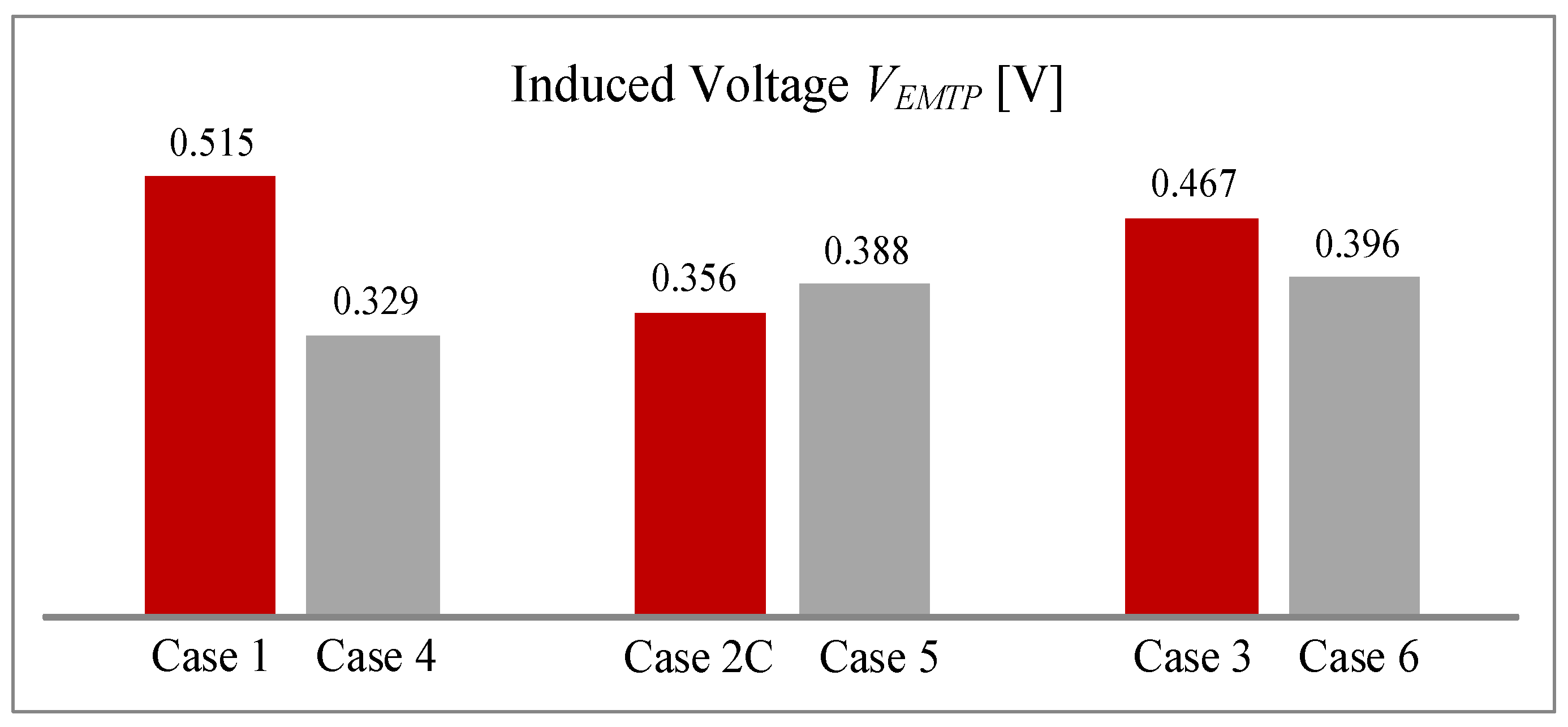
3.3. Comparison of Case SCL and DCL Studies

Figure 7 shows the induced voltages in SCL and DCL configurations with the same load condition. The induced voltage in the SCL case is larger than the induced voltage in the DCL case, except for the C-phase unbalanced load case. The Case 2C and Case 5 results indicate that the induced voltage in the DCL case is larger than the inducing side voltage and V_N (shielding side), as shown in

Table 8. Comparison of Case 2C and Case 5.

Case Study	Inducing Side	Shielding Side VG + VN (V)	Induced Voltage VP (V)
Case 2C	6.976 ∠ −4.71°	0.198 ∠ −57.54° + 6.783 ∠ 172.7°	0.353 ∠ 20.23°
Case 5	13.446 ∠ −7.7°	0.343 ∠ −88.0° + 13.697 ∠ 172.4°	0.401 ∠ −126.1°

.

Figure 8 shows that the induced voltage with the upper and lower sides of the DCL carry the same single-phase unbalanced load. The induced voltage in the DCL configuration is different than in the SCL configuration due to inductive coupling on the pipeline located at different single-phase unbalanced loads.

The induced voltage of the lower side in Case 8A–8C is larger than the induced voltage of the upper side in Case 7A–7C, due to the effect of lower side-induced voltages, which are closely arranged to the pipeline. However, the result indicates that the lower single-phase unbalanced load is smaller than the upper single-phase unbalanced load. Since the inducing and shielding side voltage magnitudes in Case 8 are smaller than the voltage magnitude in Case 7, the simulation results agree with the vector analysis shown in Table 7.

Table 9. Induced voltage according to the separation distance in SCL.

Case Study	Separation Distance (VEMTP (V))
	−90 (m)	−60 (m)	−30 (m)	0 (m)	+30 (m)	+60 (m)	+90 (m)
Case 1	0.111	0.141	0.216	1.540	0.287	0.187	0.142
Case 2A	0.099	0.136	0.236	0.332	0.533	0.336	0.250
Case 2B	0.271	0.326	0.448	0.565	0.552	0.387	0.309
Case 2C	0.207	0.275	0.434	0.177	0.341	0.213	0.156
Case 3	0.209	0.268	0.407	0.243	0.411	0.271	0.207

and

Table 10. Inducing and shielding side analysis in Case 2A of Table 9.

Separation Distance	Inducing Side Voltage (V)	Shielding Side Voltage (V)	Induced Voltage (V)
−90 (m)	4.164 ∠ −135.51°	4.118 ∠ 43.26°	0.099 ∠ −73.53°
−60 (m)	4.862 ∠ −132.86°	4.768 ∠ 45.99°	0.136 ∠ −87.79°
−30 (m)	6.037 ∠ −129.93°	5.827 ∠ 49.09°	0.236 ∠ −104.45°
0 (m)	7.086 ∠ −127.30°	7.411 ∠ 52.05°	0.332 ∠ 38.28°
+30 (m)	5.301 ∠ −129.94°	5.827 ∠ 49.09°	0.533 ∠ 39.34°
+60 (m)	4.438 ∠ −133.13°	4.768 ∠ 45.99°	0.336 ∠ 34.56°
+90 (m)	3.874 ∠ −135.94°	4.118 ∠ 43.26°	0.250 ∠ 30.81°

show EMTP simulation results by separation distance in the SCL case. The separation distance is ±90 m between 1 km lengths of the parallel overhead distribution lines.

The induced voltage due to the inductive coupling on the pipeline located at a different unbalanced load of single-phase simulation cases, Case 2A–2C, is shown in Figure 9. The simulation results indicate that the induced voltage is negligible at the center of the ODL and the peak, where the pipeline is located at a separation distance near ±15 m, as shown in Figure 9 and Table 10.

Table 11. Induced voltage according to the separation distance in DCL.

Case Study	Separation Distance (VEMTP (V))
	−90 (m)	−60 (m)	−30 (m)	0 (m)	+30 (m)	+60 (m)	+90 (m)
Case 4	0.197	0.228	0.275	0.311	0.280	0.228	0.197
Case 5	0.202	0.237	0.303	0.542	0.289	0.235	0.202
Case 6	0.247	0.286	0.351	0.439	0.347	0.286	0.247
Case 7A	0.199	0.239	0.323	0.550	0.255	0.197	0.170
Case 7B	0.383	0.447	0.562	0.864	0.605	0.470	0.399
Case 7C	0.179	0.209	0.254	0.323	0.234	0.197	0.171
Case 8A	0.171	0.196	0.234	0.381	0.290	0.219	0.184
Case 8B	0.289	0.339	0.431	0.577	0.396	0.317	0.273
Case 8C	0.158	0.178	0.201	0.181	0.265	0.216	0.184

shows EMTP simulation results by separation distance in the DCL case. Induced voltage due to the inductive coupling on the pipeline located at a different unbalanced load of single-phase (Case 7A–7C) is shown in Figure 10.

The induced voltage has a peak value at the center of the ODL with DCL and gradually decreases as the transverse position of the pipeline increases. Therefore, when comparing SCL and DCL cases by the separation distance, SCL shows asymmetric characteristics about the y-axis, whereas DCL shows asymmetric characteristics.

4. Conclusions

This paper analyzed the induced voltage from a parallel distribution system using Carson’s formula and vector analysis. The calculation method for the induced voltage is not suitable due to the excessive errors caused by the screening factors of the neutral current.

For a more practical analysis of the induced voltage, a new analysis is needed to use the actual neutral current and to consider the overhead ground conductor and the neutral conductor in the distribution system. The shielding effect of the neutral current was verified by both calculation and vector analysis. Thus, the proposing method is demonstrated without using the screening factor.

The calculation results are verified by the EMTP simulation and vector composition method. Moreover, various case studies are analyzed according to the load conditions, separation distance, and pole types of the distribution system. In addition, the induced voltage of the DCLs has fewer EM effects than the induced voltage of the SCLs in the same load condition. From the results that did not generate very much of an error, it is expected that the proposed method can be useful to calculate the induced voltage on pipelines located close to the parallel distribution system.

References

1. Adedeji, K.; Ponnle, A.; Abe, B.; Jimoh, A.; Abu-Mahfouz, A.; Hamam, Y. A review of the effect of ac/dc interference on corrosion and cathodic protection potentials of pipelines. Int. Rev. Electr. Eng. 2018, 13, 495–508. [Google Scholar] [CrossRef] [Green Version]
2. Christoforidis, G.C.; Labridis, D.P.; Dokopoulos, P.S. A hybrid method for calculating the inductive interference caused by faulted power lines to nearby buried pipelines. IEEE Trans. Power Deliv. 2005, 20, 1465–1473. [Google Scholar] [CrossRef]
3. Gummow, R.A.; Segall, S.M.; Fieltsch, W. Pipeline AC mitigation misconceptions. In Proceedings of the Northern Area Western Conference, Calgary, AB, Canada, 15–18 February 2010. [Google Scholar]
4. Abdel-Gawad, N.M.K.; El Dein, A.Z.; Magdy, M. Mitigation of induced voltages and AC corrosion effects on buried gas pipeline near to OHTL under normal and fault conditions. Electr. Power Syst. Res. 2015, 127, 297–306. [Google Scholar] [CrossRef]
5. Kaboli, A.; Hr, S.; Al Hinai, A.; Al-Badi, A.; Charabi, Y.; Al Saifi, A. Prediction of Metallic Conductor Voltage Owing to Electromagnetic Coupling Via a Hybrid ANFIS and Backtracking Search Algorithm. Energies 2019, 12, 3651. [Google Scholar] [CrossRef] [Green Version]
6. NACE SP0177-2014. Mitigation of Alternating Current and Lightning Effects on Metallic Structures and Corrosion Control Systems; Nace International: Houston, TX, USA, 2014. [Google Scholar]
7. International Organization for Standardization. Corrosion of Metals and Alloys-Determination of AC Corrosion-Protection Criteria; Standard EN ISO 18086:2017; International Organization for Standardization: Geneva, Switzerland, 2017. [Google Scholar]
8. Ouadah, M.; Touhami, O.; Ibtiouen, R.; Benlamnouar, M.F.; Zergoug, M. Corrosive effects of the electromagnetic induction caused by the high voltage power lines on buried X70 steel pipelines. Int. J. Electr. Power Energy Syst. 2017, 91, 34–41. [Google Scholar] [CrossRef]
9. Lucca, G. AC interference from faulty power cables on buried pipelines: A two-step approach. IET Sci. Meas. Technol. 2021, 15, 25–34. [Google Scholar] [CrossRef]
10. Martins-Britto, A.G.; Rondineau, S.R.M.J.; Lopes, F.V. Power Line Transient Interferences on a Nearby Pipeline Due to a Lightning Discharge. In Proceedings of the International Conference on Power Systems Transients (IPST 2019), Perpignan, France, 16–20 June 2019. [Google Scholar]
11. Martins-Britto, A.; Moraes, C.M.; Lopes, F.V.; Rondineau, S. Low-frequency Electromagnetic Coupling Between a Traction Line and an Underground Pipeline in a Multilayered Soil. In Proceedings of the 5th Workshop on Communication Networks and Power Systems (WCNPS 2020), IEEE Xplore, Brasília, Brazil, 12–13 November 2020; pp. 1–6. [Google Scholar]
12. Peppas, G.D.; Papagiannis, M.-P.; Koulouridis, S.; Pyrgioti, E.C. Induced Voltage on an Aboveground Natural Gas/Oil Pipeline Due to Lightning Strike on a Transmission Line. In Proceedings of the 2014 International Conference on Lightning Protection (ICLP), Shanghai, China, 11–18 October 2014; pp. 461–467. [Google Scholar]
13. Popoli, A.; Cristofolini, A.; Sandrolini, L. A numerical model for the calculation of electromagnetic interference from power lines on nonparallel underground pipelines. Math. Comput. Simul. 2021, 183, 221–233. [Google Scholar] [CrossRef]
14. Moraes, C.M.; Martins-Britto, A.G.; Felipe, V. Electromagnetic Interferences Between Power Lines and Pipelines Using EMTP Techniques. In Proceedings of the 2020 Workshop on Communication Networks and Power Systems (WCNPS) Communication Networks and Power Systems (WCNPS), 2020 Workshop, Brasilia, Brazil, 1–6 November 2020. [Google Scholar]
15. Heo, J.Y.; Seo, H.C.; Lee, S.J.; Kim, Y.S.; Kim, C.H. A Simulator for Calculating Normal Induced Voltage on Communication Line. J. Electr. Eng. Technol. 2014, 9, 1394–1400. [Google Scholar] [CrossRef] [Green Version]
16. Hiroshi, I.; Akihiro, A.; Yuji, H. An investigation of induced voltages to an underground gas pipeline from an overhead transmission line. Electr. Eng. 2008, 164, 43–50. [Google Scholar]
17. Leuven EMTP Center. Alternative Transients Program ATP Rule Book; EEUG, Canadian/American EMTP User Group: Portland, OR, USA, 1992. [Google Scholar]
18. Popoli, A.; Sandrolini, L.; Cristofolini, A. Reduction in the Electromagnetic Interference Generated by AC Overhead Power Lines on Buried Metallic Pipelines with Screening Conductors. Electricity 2021, 2, 316–329. [Google Scholar] [CrossRef]
19. Park, K.W.; Seo, H.C.; Kim, C.H.; Kim, C.H.; Jung, C.S.; Yoo, Y.P.; Lim, Y.H. Analysis of the Neutral Current for Two-Step-Type Poles in Distribution Lines. IEEE Tran. Power Deliv. 2009, 24, 1483–1489. [Google Scholar] [CrossRef]
20. Oka, K.; Koizumi, S.; Oishi, K.; Yokota, T.; Uemura, S. Analysis of a neutral grounding method for a three phase four-wire 11.4 kV distribution system. In Proceedings of the Transmission and Distribution Conference and Exhibition 2002: Asia Pacific. IEEE/PES, Yokohama, Japan, 6–10 October 2002; Volume 2, pp. 998–1003. [Google Scholar]
21. Kim, H.S.; Rhee, S.B.; Yeo, S.M.; Kim, C.H.; Lyn, S.H.; Kim, S.A.; Weon, B.J. Calculation of an Induced Voltage on Telecommunication Lines in Parallel Distribution Lines. Trans. KIEE 2008, 57, 1688–1695. [Google Scholar]
22. National Radio Research Agency. The Technical Regulation on Detailed Calculation Methods of Power Induction Voltages; RRA Notice No. 2014-11; National Radio Research Agency: Naju, Korea, 2014. [Google Scholar]
23. Kersting, W.H. The Modeling and Analysis of Parallel Distribution Lines. IEEE Trans. Ind. Appl. 2006, 42, 1126–1132. [Google Scholar] [CrossRef]
24. Electric Power Research Institute. EPRI AC Transmission Line Reference Book—200 kV and Above; Electric Power Research Institute: Washington, DC, USA, 2014. [Google Scholar]
25. Papadopoulos, T.A.; Apostolidis, A.K.; Chrysochos, A.I.; Christoforidis, G.C. Frequency-Dependent Earth Impedance Formulas Between Overhead Conductors and Underground Pipelines. In Proceedings of the IEEE International Conference on Environment and Electrical Engineering and 2019 IEEE Industrial and Commercial Power Systems Europe (EEEIC/I&CPS Europe), Genova, Italy, 11–14 June 2019; pp. 11–14. [Google Scholar]
26. Amtani, A.; Hosakawa, Y. EMTP Simulations and Theoretical Formulation of Induced Voltages to Pipelines from Power Lines; IPST: Lyon, France, 2007. [Google Scholar]
Figure 1. Induced voltage calculation of SCL.
Energies 14 08536 g001
Figure 2. Induced voltage calculation of DCL.
Energies 14 08536 g002
Figure 3. Configurations of distribution lines and pipelines. (a) SCL. (b) DCL.
Energies 14 08536 g003
Figure 4. Configuration of the pipelines; rg1 = 191.3 (mm), rg2 = 203.2 (mm), rg3 = 206.4 (mm); ρg = 1.59 × 10⁻⁷ (Ω m), μg = 280, εg = 2.30.
Energies 14 08536 g004
Figure 5. Vector diagram of SCL (Case 2A, Case 2C), where VP is multiplied by five for clarity, as shown in the legend.
Energies 14 08536 g005
Figure 6. Vector diagram of DCL (Case 7B, Case 8B), where VP is multiplied by five for clarity and illustrative purposes.
Energies 14 08536 g006
Figure 7. Comparison of SCL and DCL.
Energies 14 08536 g007
Figure 8. Comparison of single-phase unbalanced load in DCL.
Energies 14 08536 g008
Figure 9. Induced voltage according to the separation distance in SCL.
Energies 14 08536 g009
Figure 10. Induced voltage according to the separation distance in DCL.
Energies 14 08536 g010