LQR and Fuzzy Logic Control for the Three-Area Power System

Abstract

The three-area power system is widely considered a suitable example to test load frequency control of the distributed generation system. In this article, for such a system, for the power stabilization task, we introduce two controllers: Linear Quadratic Regulator (LQR), which is model-based, and Fuzzy Logic Controller (FLC), which is data-based. The purpose is to compare the two approaches from the point of view of (i) ease of implementation and tuning, and (ii) robustness to changes in the model. The model, together with controls strategies, has been implemented in the MATLAB software. Then, it has been tested for different simulation scenarios, taking into account the disturbances and faulty tie-lines between areas. Various quality measures allow to compare the performance of each control strategy. The comparison in terms of parameter change and load disturbances prompt us to propose suitable metrics and advice notes on the application of each controller.

1. Introduction

Increased flexibility and intelligence in the optimization and control of modern power systems seem to be necessary to maintain a generation–load balance in presence of various disturbances. This issue has become more serious today due to the use of a large number of microgrids (MGs). The MGs often utilize different means to generate electricity, the parameters of which naturally fluctuate. The presence of these uncertainties and fluctuations means that the conventional controllers are not efficient enough to ensure the stability and to provide a proper performance for the different operating conditions in power systems [1]. Off-the-shelf advanced control toolboxes need further improvements and tuning to demonstrate significant benefits for this type of applications.

Multi-area power network system usually consists of interconnected subsystems or control areas linked by tie-lines or High-Voltage Direct Current (HDVC) links. The individual areas consist of generator or generators responsible for their load and scheduled interchanges with nearby areas [2]. Load frequency control (LFC) is used in power systems for the maintenance of the load–generation balance. The angular speed of the rotor of the generator is a function of the mismatch between the input mechanical power and the output electrical power [3]. The LFC allows for the controlled exchange of power to assist in the overall robustness of operation while simultaneously allowing economic power generation [4]. A load frequency controller is required to ensure some level of control over the net power flow on the tie-lines.

In interconnected power system operation and design, Automatic Generation Control (AGC) is one of the significant control issues these days because of the growing size, emerging renewable energy sources, and complexity of power systems [5]. AGC performs a significant contribution towards maintaining a generation–load balance with respect to various disturbances. In fact, AGC is utilized to balance the changes in the generation and load to restore frequency at the initial value and to meet tie-line flows. AGC is mainly responsible for power interchange, frequency control, and economic dispatch. In many practical applications, some conventional control approaches have been used for AGC such as PID, PI, and optimal control methods, but these controllers have some limitations including difficulty in dealing with system uncertainties, external disturbances, and the speed of response [6]. Although some control methods such as robust control [7], MPC [8,9], and PI control [10] successfully overcome many AGC issues, a key problem is that the uncertainties are not explicitly used in the control design. This issue has been investigated in [11] by proposing a new optimal controller for AGC in the presence of non-Gaussian wind power uncertainty.

Load Frequency Control (LFC), as an integral part of the power system operation and control, has been proposed to cater for parametric changes or uncertainties in the system and performance improvement of the multi-area power systems [5]. The LFC is an integral part of the multi-area power systems as it is responsible for the load–generation balance and simultaneously regulating the output power of each generator at preset levels. The LFC is becoming more challenging and significant due to increasing penetration level of renewable energy in power production in modern power systems. This issue and effects of renewable distributed generations, such as photovoltaic stations and wind turbine generator, on LFC has been rarely investigated [12,13,14,15,16]. Additionally, many contributions in the literature aimed towards the optimization of LFC for power systems are mostly based on conventional control methods. Usually such controllers does not provide a proper performance with uncertainties and fluctuations caused by renewable distributed generations [1]. Multiple control schemes have been proposed for the design of an LFC, mainly the proportional and integral (PI) control [17], proportional integral derivative (PID) control [18,19,20,21], model predictive control (MPC) [8,22,23], robust MPC [24] robust control scheme [25], neural network control method [26], and sliding mode control scheme [27,28,29]. A decentralized adaptive back-stepping excitation controller has been designed in [30] for stability enhancement of multi-machine power systems. The adaptive control has been used in [2] to develop a robust LFC scheme for a multi-area power system with parametric uncertainties. The sliding mode control has been used in [31] to design a discrete LFC for multi-area power systems with matched and unmatched uncertainties, and a sliding mode load frequency controller (SMLFC) has been designed for a power system with mismatched uncertainty in [32]. The common problem with sliding mode control is chattering phenomenon due to discontinuous terms, and different approaches have been proposed for its reduction [33]. The proportional integral derivative (PID) LFC has been designed together with the robust technique in [34] for multi-machine power systems. However, the generation rate constraint, unmatched uncertainty, and resource variation were not studied in those researches. Furthermore, most of the research only considered a single area power system.

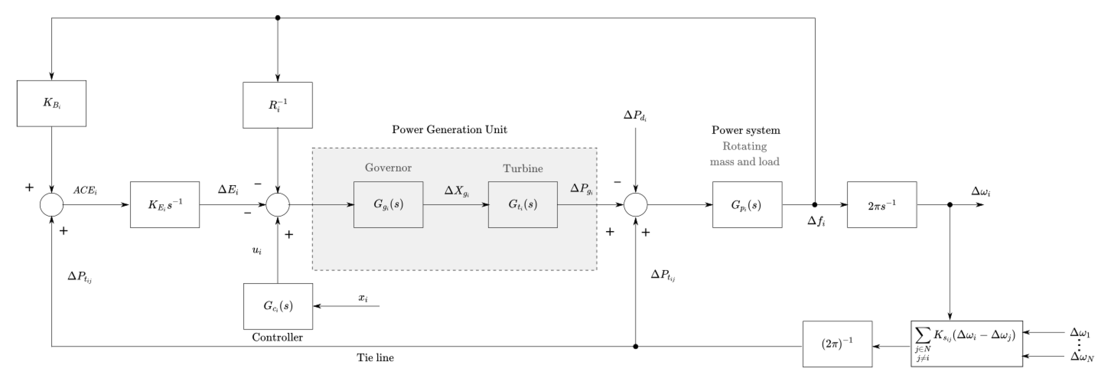
Tie-line Bias control has been utilized as the desired control scheme in North America for the past 75 years. The term Area Control Error (ACE) was introduced in the early 1950s for the specific implementation of coordinated Tie Line Bias control which is now widely used throughout the world. The Balancing Area’s ACE is calculated by AGC from interchange and frequency data. The ACE informs if that the system is in balance or requires some adjustments to generation. The ACE represented in MW comprises the difference between the Balancing Authority Area’s Actual Net Interchange and its Scheduled Net Interchange, plus its Frequency Bias Setting obligation, plus correction for any known meter error. In the Western Interconnection, reporting ACE consists of Automatic Time Error Correction [35]. Much effort has been made to use the concept of ACE for the LFC in the literature. The concept of ACE based on frequency and tie-power deviation, inadvertent interchange, and time error has been utilized in [36] to control the battery energy storage system. In [37], in order for bounding the system frequency within a target range, a concept of ACE has been utilized.

Linear Quadratic Regulator (LQR) is an effective optimal control method based on the selection of feedback gain in a manner to minimize the cost function [38,39]. The LQR is an optimal control approach based on a cost function which contains weighting matrices to achieve a desired behaviour [40]. The LQR is applicable for optimizing multiple input multiple output systems and its properties depend on the appropriate selection of matrix that reflects the weighting on the non-zero penalties on the states and the matrix which corresponds to the weightings on the penalties on process inputs [41]. The LQR enables stability in systems and it allows for voltage regulation and load sharing simultaneously [42,43]. However, the robustness of the LQR control scheme is poor. In [44], an LQR has been proposed for the inner voltage control loop in an islanded microgrid. A robust control scheme based on LQR-fuzzy logic was designed in [45,46] for a single area power system.

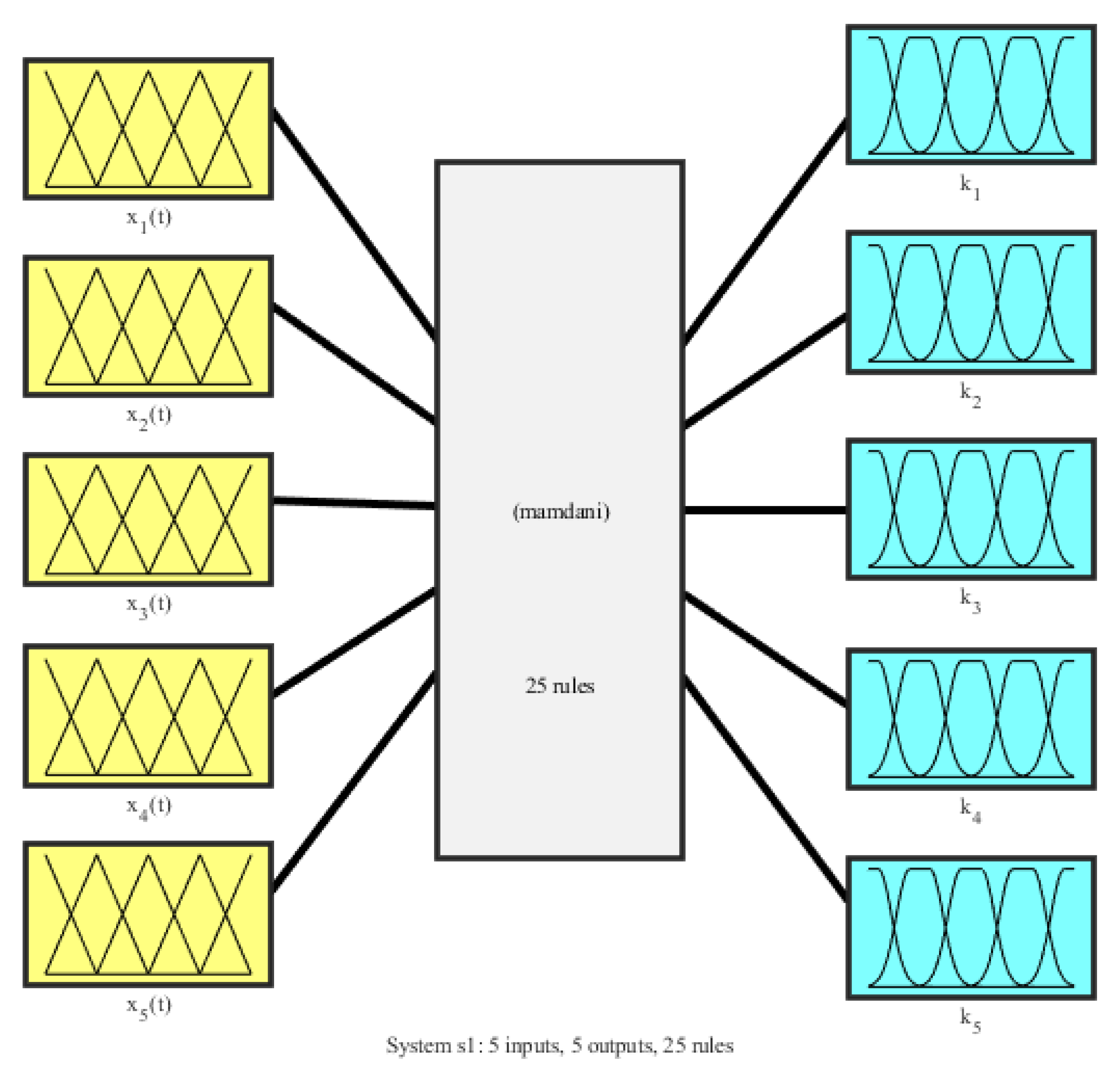
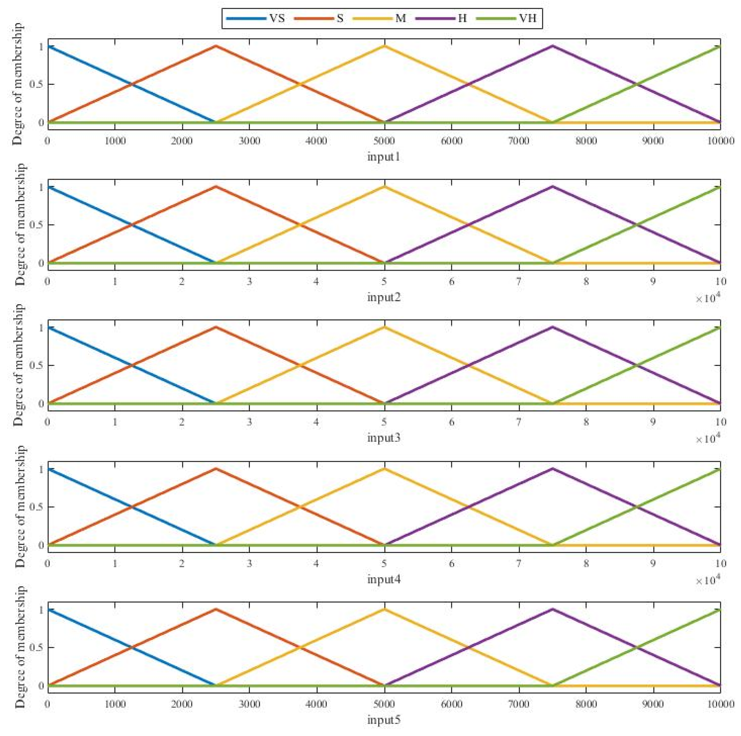
Fuzzy logic, proposed by Lotfi A. Zadeh in 1965 is a model-free approach utilizing linguistic variables to imitate the human operator’s way of thinking [47]. As the fuzzy logic is a model-free approach, it has no requirement on the model structure or the knowledge of the rules controlling the relationship between the process inputs and outputs of the system [48]. This makes it suitable for complicated systems whose mathematical models are difficult to establish. Fuzzy logic, however, has the disadvantage of the requirement of a vast information to compensate for system parameter changes or when there is an increase in the number of inputs [49,50]. Fuzzy logic integrated with sliding mode control [51] or back-stepping provides an effective way to increase the robustness of the controller with respect to parametric uncertainties and external disturbances [52].

Aim of the Paper

The paper aims to analyze and compare the quality of LQR and Fuzzy Logic Controller in three area power distribution systems. While LQR controller for power generation is a relatively well established technique, it relies on knowledge of the model of the system in order to build a state-space representation. On the other hand, the fuzzy control is gaining more interest recently, because it does not require a precise state-space model of the controlled system. Therefore, the idea to compare the two approaches taking into consideration: (i) ease of implementation and tuning of the controller and (ii) robustness of the control to changes in the parameters of the system. To this end, three simulation scenarios have been selected to progressively test both controllers against increasingly difficult control tasks. The first two scenarios test the dynamic responses of the system whereas the third scenario assumes changes in the system model, caused by decoupling of the areas, which are not visible to the controller. The model and the controls strategies have been implemented in the MATLAB software. The implementation is available at the MATLAB file exchange platform [53]. The performance control strategies is compared using various quality measures.

Fuzzy logic has been integrated with the adaptive control technique to design a LFC for a multi-area power system [54]. In [55], fuzzy control has been used to design and implement the energy management system (EMS) for a DC microgrid. In [56], a generalized droop control (GDC) has been firstly designed to minimize the reactive power and active effects on the frequency and voltage. Then, a fuzzy logic has been employed for tuning the secondary control parameters (PI) and the GDC. The results reveal that the proposed fuzzy logic controllers outperform non-fuzzy control method.

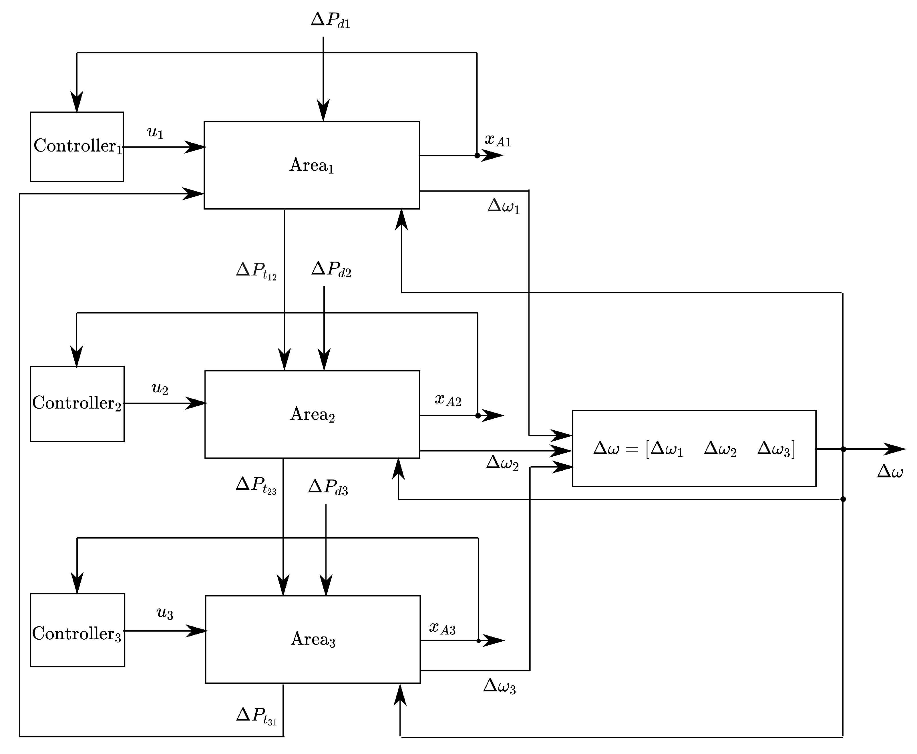
The paper is organized as follows. The first part of the paper describes a general mathematical model of the multi-area generation network and then narrows it down to the model of three coupled areas. Furthermore, it describes the theoretical background of the LQR and the proposed fuzzy controller and explains their implementation for the model of the 3-area network. The Simulation and Results chapter describes simulation scenarios and controller parameters. This is followed by the simulation results presented in graphical and tabular forms. This chapter also contains a comparison of control quality for the algorithms and the scenarios. The Discussion section shows the advantages and disadvantages of methods in terms of stability, accuracy, and robustness. The overall conclusions and discussion of possible directions of future work are provided in the Conclusions section.

2. Materials and Methods

2.1. Mathematical Model of the Multi-Area Power Generation Network

Figure 1 shows a model for the i-th area of an N-area power system. In the case considered in this paper, each area consists of governor-turbine energy generator with the non-reheat steam turbine. It is connected in the closed loop with the power system. Although a power system is nonlinear, the use of the linearized model is permissible in the LFC problem because only small changes in load are expected during its normal operation. Therefore, each element is described with the corresponding transfer function as follows:

Governor transfer function

$$G_{gi}={\displaystyle \frac{1}{1+s{T}_{Gi}}}$$

(1)

where $T_{Gi}$—governor time constant.

Turbine transfer function

$$G_{ti}={\displaystyle \frac{1}{1+s{T}_{Ti}}}$$

(2)

where $T_{Ti}$—turbine time constant.

Generator transfer function

$$G_{Pi}={\displaystyle \frac{K_{Pi}}{1+s{T}_{Pi}}}$$

(3)

where $K_{Pi}$—power system gain and $T_{Pi}$—power system time constant.

The N-area power system is described with the following equations:

$$\begin{array}{cc}\hfill \Delta {\dot{f}}_i\left(t\right)=& -\frac{1}{T_{p_i}}\Delta f_i\left(t\right)+\frac{K_{p_i}}{T_{p_i}}\Delta P_{g_i}\left(t\right)-\frac{K_{p_i}}{T_{p_i}}\Delta P_{d_i}\left(t\right)\hfill \\ \hfill & -\frac{K_{p_i}}{2\pi T_{p_i}}\sum _{j=1,j\ne i}^N{K}_{sij}\left\{\Delta {\delta }_i\left(t\right)-\Delta {\delta }_j\left(t\right)\right\}\hfill \end{array}$$

(4)

$$\Delta {\dot{P}}_{g_i}\left(t\right)=-\frac{1}{T_{t_i}}\Delta P_{g_i}\left(t\right)+\frac{1}{T_{t_i}}\Delta X_{g_i}\left(t\right)$$

(5)

$$\begin{array}{cc}\hfill \Delta {\dot{X}}_{g_i}\left(t\right)=& \frac{-1}{R_i{T}_{G_i}}\Delta f_i\left(t\right)-\frac{1}{T_{G_i}}\Delta X_{g_i}\left(t\right)-\hfill \\ & \frac{1}{T_{G_i}}\Delta E_i\left(t\right)+\frac{1}{T_{G_i}}{u}_i\left(t\right)\hfill \end{array}$$

(6)

$$\begin{array}{cc}\hfill \Delta {\dot{E}}_i\left(t\right)=& K_{E_i}\left[K_{B_i}\Delta f_i\left(t\right)+\right.\hfill \\ & +\left.\frac{1}{2\pi }\sum _{j=1,j\ne i}^N{K}_{sij}\left\{\Delta {\delta }_i\left(t\right)-\Delta {\delta }_j\left(t\right)\right\}\right]\hfill \end{array}$$

(7)

$$\Delta {\dot{\delta }}_i\left(t\right)=2\pi \Delta f_i\left(t\right)$$

(8)

where $i=1,\dots ,N$ is the area number and N—number of the areas.

Equations (4)–(8) can be represented in state space form as

$${\dot{x}}_i\left(t\right)=A_i{x}_i\left(t\right)+B_i{u}_i\left(t\right)+\sum _{\genfrac{}{}{0pt}{}{j=1}{j\ne i}}^N{E}_{ij}{x}_j\left(t\right)+F_i\Delta P_{d_i}\left(t\right)$$

(9)

where

$$A_i=\left[\begin{array}{ccccc}-\frac{1}{T_{p_1}}& \frac{K_{p_i}}{T_{p_i}}& 0& 0& -\frac{K_{p_i}}{2\pi T_{p_i}}\sum _{\genfrac{}{}{0pt}{}{j=1}{j\ne i}}^N{K}_{sij}\\ 0& -\frac{1}{T_{T_i}}& \frac{1}{T_{T_i}}& 0& 0\\ -\frac{1}{R_i{T}_{G_i}}& 0& -\frac{1}{T_{G_i}}& -\frac{1}{T_{G_i}}& 0\\ K_{E_i}{K}_{B_i}& 0& 0& 0& \frac{K_{E_i}}{2\pi }\sum _{\genfrac{}{}{0pt}{}{j=1}{j\ne i}}^N{K}_{sij}\\ 2\pi & 0& 0& 0& 0\end{array}\right]$$

(10)

$$E_{ij}=\left[\begin{array}{ccccc}0& 0& 0& 0& \frac{K_{p_i}}{2\pi T_{p_i}}{K}_{sij}\\ 0& 0& 0& 0& 0\\ 0& 0& 0& 0& 0\\ 0& 0& 0& 0& -\frac{K_{E_i}}{2\pi }{K}_{sij}\\ 0& 0& 0& 0& 0\end{array}\right]$$

(11)

$$B_i={\left[\begin{array}{ccccc}0\hfill & 0\hfill & \frac{1}{T_{G_i}}\hfill & 0\hfill & 0\hfill \end{array}\right]}^T$$

(12)

$$F_i={\left[\begin{array}{ccccc}-\frac{K_{p_i}}{T_{p_i}}& 0& 0& 0& 0\end{array}\right]}^T$$

(13)

$$x_i\left(t\right)={\left[\begin{array}{ccccc}\Delta f_i\left(t\right)\hfill & \Delta P_{g_i}\left(t\right)\hfill & \Delta X_{g_i}\left(t\right)\hfill & \Delta E_i\left(t\right)\hfill & \Delta {\delta }_i\left(t\right)\hfill \end{array}\right]}^T$$

(14)

where $x_i\left(t\right)\in {\Re }^{n_i}$—the state vector; $x_j\left(t\right)\in {\Re }^{n_j}$—the adjacent area state vector of $x_i\left(t\right)$; $u_i\left(t\right)\in {\Re }^{m_i}$—the control vector; $\Delta P_{d_i}\left(t\right)\in {\Re }^{k_i}$—the vector of load disturbance; $\Delta f_i\left(t\right)$, $\Delta P_{g_i}\left(t\right)$, $\Delta X_{g_i}\left(t\right)$, $\Delta {\mathrm{E}}_i\left(t\right)$ and $\Delta {\delta }_i\left(t\right)$—state variables, i.e., the incremental deviation in frequency (Hz), generator output (p.u. MW), governor valve position (p.u. MW), integral control and rotor angle, respectively; $K_{p_i}$, $R_i$, $K_{E_i}$, and $K_{B_i}$ are the power system and machines gain, speed regulation coefficient (p.u. MW ${}^{-1}$), integral control gain, and frequency bias factor, respectively; $T_{p_i}$, $T_{t_i}$, and $T_{G_i}$ are the time constants in (sec) of power system and machines, turbine and governor, respectively; $K_{s_{ij}}$ is the interconnection tie line gain between area i and $j(j\ne i)$. The dimensions of the i-th area matrices in (9) are $A_i\in {\Re }^{n_i\times n_i}$, $E_{ij}\in {\Re }^{n_i\times n_j}$, $B_i\in {\Re }^{n_i\times m_i}$, $F_i\in {\Re }^{n_i\in k_i}$.

2.2. Three-Area Model

The three-area model considered in this paper is described with parameters given in

Table 1. Parameters of the 3-area model.

Parameter	$\mathit{i}=1$	$\mathit{i}=2$	$\mathit{i}=3$
$K_{B_i}$	0.41	0.37	0.40
$K_{E_i}$	0.15	0.15	0.12
$R_i$	2.4	2.7	2.5
$K_{p_i}$	120	112.5	115
$T_{p_i}$	20	25	20
$T_{G_i}$	0.08	0.072	0.07
$T_{t_i}$	0.3	0.33	0.35
$K_{s_{ij}}$	$j=1$	$j=2$	$j=3$
$i=1$	0.55	0.55	0.55
$i=2$	0.65	0.65	0.65
$i=3$	0.545	0.545	0.545

.

The block diagram of the considered in the paper control system for three-area power generation system is given in Figure 2. In this paper, we consider a case of individual control system for each area. The control in each area is based on measurements in this area only, plus agglomerated information about the frequency deviations.

2.3. Description of Control Algorithms

2.3.1. Linear-Quadratic Regulator—LQR

In the case of the Linar-Quadratic Regulator, the optimal control is used minimizing the following cost function:

$$J_{\mathrm{LQR}}={\int }_0^{\infty }\left({\parallel x\left(t\right)\parallel }_Q^2+{\parallel u\left(t\right)\parallel }_R^2\right)$$

(15)

where $Q\in {\Re }^{n_x\times n_x}$—symmetric non-negative definite state weight matrix and $R\in {\Re }^{n_u\times n_u}$—symmetric positive definite control signal weight matrix. In most cases, matrices Q and R are diagonal.

The optimal state-feedback LQR controller has a form of the matrix gain as follows:

$$u\left(t\right)=-K_{LQR}x\left(t\right),K_{LQR}\in {\Re }^{n_u\times n_x}$$

(16)

For the set of the time-invariant matrices A, B, Q, and R, the control matrix gain $K_{LQR}$ in (16) minimizing the cost function (15), can be calculated as

$$K_{LQR}={(R+B^{T}PB)}^{-1}{B}^{T}PA$$

(17)

where P is a solution of the following algebraic Ricatti equation:

$$P=Q+A^T(P-PB{(R+B^{T}PB)}^{-1}{B}^{T}P)A$$

(18)

Therefore, the solution of the LQR problem is the state-feedback control matrix (17).

In the LQR controller design the coefficients of diagonal weight matrices Q, and R should be chosen. The initial values can be selected using the following Bryson’s rule  [57]

$$Q_{ii}={\displaystyle \frac{1}{x_{i\mathrm{acc}}^2}},i=1,\dots ,n_x,R_{jj}={\displaystyle \frac{1}{u_{j\mathrm{acc}}^2}},j=1,\dots ,n_u$$

(19)

where $x_{i\mathrm{acc}}$, $u_{j\mathrm{acc}}$ are the maximum acceptable values of the i-th internal state and j-th control signal, respectively.

Maximum acceptable values in (19) depend on the additional requirements of the proposed control system. In case of no limitations, the corresponding weights based on Bryson’s rule should be equal to 0.

2.3.2. Fuzzy Controller

The problems with the model uncertainty and disturbances can be addressed using the fuzzy logic controller. This method is based on describing the behavior of a Multi-Input Multi-Output (MIMO) dynamical system using fuzzy inference rules. It allows to build controller with the use of fuzzy rules, obtained either from domain experts domain experts or observed control actions or both. The advantage is a lack of the requirement of a mathematical model of the physical phenomena describing multi-area power system.

In this section, the fuzzy logic controller (FLC) is applied to the three area power generation system. As mentioned, FLC is not model-based, thus it cannot take advantage of the knowledge of the model parameters. However, it is easy to implement. By comparing the output of the system and the desired values, based on observations, it can provide us with desired results. Here, for each area, FLC has been considered individually. The absolute values of 5 states of the system have been used as inputs for FLC’s for each area. Then, the fuzzy inference is performed by defining a membership function and fuzzy rules. Fuzzy rules are based on cause-effect relationships in the system which is defined here based on the observation of the system behaviour.

The fuzzy controller provides us with 5 different outputs, $k_{i,j}$; $i=(1,2,3,4,5)$. These outputs, $k_i$, are gains of the controller, i.e.,

$$u_j=-K_{FLC,j}{x}_j;K_{FLC,j}={[k_1\cdots k_5]}_j$$

(20)

where j is the area number.

Note that the concept of state controller has been considered to design FLC where the gain of controller $k_i$ is obtained using fuzzy logic rules. The conditions for all fuzzy simulation are considered as follows: Fuzzy system: Mamdani; And method: min; Or method: Max; Implication: min; Aggregation: sum; Defuzzification: entroid. The considered fuzzy rules are provided in

Table 2. Fuzzy rules for each area.

If	Is	Then	Is
$x_i\left(t\right)$	Very Small (VS)	$k_i$	Small (S)
$x_i\left(t\right)$	Small (S)	$k_i$	Medium (M)
$x_i\left(t\right)$	Medium (M)	$k_i$	High (H)
$x_i\left(t\right)$	High (H)	$k_i$	Very High (VH)
$x_i\left(t\right)$	Very High (VH)	$k_i$	Very High (VH)

, for $i=(1,2,3,4,5)$. The structure of fuzzy system is shown in Figure 3.

3. Simulations and Results

3.1. Simulation Model: Three-Area AGC Systems

Three-area AGC was simulated using MATLAB software and ode45 solver. The control signal of the LQR controller was calculated based on LQR function from Control System Toolbox. The control signal of the FLC controller was calculated using Fuzzy Logic Toolbox.

3.2. Simulation Scenarios

Three different scenarios are proposed for the comparison of LQR and fuzzy controllers. Different initial conditions, disturbances, and parameters changes of the controlled three-area power system are considered. It shall allow to draw conclusions on the robustness of the proposed solutions.

• The simulation scenario 1 is the analysis of the control system response to non zero initial conditions, i.e., $\Delta f_1=0.15$, $\Delta f_2=0$ and $\Delta f_3=-0.1$.

• The simulation scenario 2 is the analysis of the control system response to non zero initial conditions, i.e., $\Delta f_1=0.15$, $\Delta f_2=0$ and $\Delta f_3=-0.1$ and the step change in the disturbance load, i.e., $\Delta P_{d1}=0.02$, $\Delta P_{d2}=0.015$, and $\Delta P_{d3}=0.01$.

• The simulation scenario 3 is the analysis of the decoupled control system response to non zero initial conditions, i.e., $\Delta f_1=0.15$, $\Delta f_2=0$ and $\Delta f_3=-0.1$ and the step change in the disturbance load, i.e., $\Delta P_{d1}=0.02$, $\Delta P_{d2}=0.015$, $\Delta P_{d3}=0.01$. The system decoupling is achieved by substituting the zero values for $K_{sij}$ parameters.

All scenarios were repeated for both controllers: (1) LQR controller with the exact model parameters and (2) Fuzzy Logic Controller.

Controller Gains

As it is presented in the results of different scenarios, the controller gains differ, depending on the algorithms. However, the gains vectors for each controller have the same size, i.e., $dim\left(K_{LQR}\right)=dim\left(K_{FLC}\right)=5$, and are the weights of the elements of the same state vector $x\in R^{5\times 1}$. Therefore, the algorithms are compared here as it will allow to better understanding of the performance of the control system.

The input membership function of the FLC for different scenarios is given in Figure 4. The output membership functions of the FLC for scenario 1 are given in Figure 5 and for scenarios 2 and 3 are given in Figure 6. Note that the output membership functions of the FLC for scenario 1 compared to the one for scenarios 2 and 3 are different which is considered based on the observation of the results to enhance the accuracy.

• Initial value for area 1: $x_1\left(0\right)=0.15,x_2\left(0\right)=0.1,x_3\left(0\right)=0.2,x_4\left(0\right)=0.5,x_5\left(0\right)=0$
• Initial value for area 2: $x_1\left(0\right)=-0.1,x_2\left(0\right)=0.1,x_3\left(0\right)=0.15,x_4\left(0\right)=0,x_5\left(0\right)=0.1$
• Initial value for area 3: $x_1\left(0\right)=0.2,x_2\left(0\right)=0.1,x_3\left(0\right)=0.1,x_4\left(0\right)=0.1,x_5\left(0\right)=0.1$

Table 3. Controller gains, Area 1.

LQR
Scenario	$k_1$	$k_2$	$k_3$	$k_4$	$k_5$
S1, S2, S3	2.1747	2.6671	0.8500	0.4142	0.2574
FLC
Scenario	$k_1$	$k_2$	$k_3$	$k_4$	$k_5$
S1	70.0000	110.4000	7.4400	4.5000	8.2700
S2	177.8000	78.0000	4.1600	0.2500	32.1000
S3	80.0000	110.2000	7.4000	4.5000	8.3000
Scenario	$k_1{}_{min}$	$k_2{}_{min}$	$k_3{}_{min}$	$k_4{}_{min}$	$k_5{}_{min}$
S1	43.8000	66.8000	2.2500	2.2500	8.2600
S2	170.7000	78.0000	3.2000	0.2500	32.1000
S3	40.0000	68.0000	2.2500	2.2500	8.3000
Scenario	$k_1{}_{max}$	$k_2{}_{max}$	$k_3{}_{max}$	$k_4{}_{max}$	$k_5{}_{max}$
S1	110.6000	111.2000	8.2700	4.5000	8.2700
S2	186.5000	78.0000	4.5200	0.2500	32.1000
S3	110.8000	111.6000	8.3000	4.5000	8.3000

,

Table 4. Controller gains, Area 2.

LQR
Scenario	$k_1$	$k_2$	$k_3$	$k_4$	$k_5$
S1, S2, S3	2.3917	2.4389	0.7505	0.4142	0.2043
FLC
Scenario	$k_1$	$k_2$	$k_3$	$k_4$	$k_5$
S1	70.8000	110.4000	7.4400	8.3600	8.2800
S2	177.7000	77.9000	4.1000	0.9000	30.4000
S3	71.0000	110.2000	7.5000	8.3200	4.5000
Scenario	$k_1{}_{min}$	$k_2{}_{min}$	$k_3{}_{min}$	$k_4{}_{min}$	$k_5{}_{min}$
S1	42.8000	66.8000	2.2500	8.3600	8.2600
S2	170.7000	77.6000	4.5000	0.9000	30.4000
S3	39.5000	68.0000	2.2500	8.3200	2.2500
Scenario	$k_1{}_{max}$	$k_2{}_{max}$	$k_3{}_{max}$	$k_4{}_{max}$	$k_5{}_{max}$
S1	110.6000	111.6000	8.3000	8.3700	8.2800
S2	186.5000	79.0000	3.2000	0.9000	32.1000
S3	110.8000	111.5000	8.3000	8.3700	8.26000

and

Table 5. Controller gains, Area 3.

LQR
Scenario	$k_1$	$k_2$	$k_3$	$k_4$	$k_5$
S1, S2, S3	2.2507	2.8882	0.7763	0.4142	0.2381
FLC
Scenario	$k_1$	$k_2$	$k_3$	$k_4$	$k_5$
S1	70.9000	110.1000	7.5000	2.2500	8.3300
S2	177.8000	78.0000	4.1600	0.2600	32.3000
S3	71.0000	110.2000	7.4700	2.2500	8.2600
Scenario	$k_1{}_{min}$	$k_2{}_{min}$	$k_3{}_{min}$	$k_4{}_{min}$	$k_5{}_{min}$
S1	30.000	110.1000	6.7600	2.2500	8.2600
S2	145.5000	74.5000	2.9000	0.2500	32.3000
S3	30.000	110.1000	6.7600	2.2500	7.5000
Scenario	$k_1{}_{max}$	$k_2{}_{max}$	$k_3{}_{max}$	$k_4{}_{max}$	$k_5{}_{max}$
S1	72.8000	111.6000	7.5000	2.2500	8.3800
S2	183.1000	79.0000	4.6000	0.2600	32.5000
S3	73.5000	111.6000	7.7000	2.2500	8.3700

give the values of the calculated of the LQR controller, and the range $[k_{FLC,i}{}_{min},k_{FLC,i}{}_{max}],i=1,\dots ,5$ of the adaptive changes of FLC controller parameters, and final values of FLC controller parameters $\left[k_{FLC,i}\right],i=1,\dots ,5$. Furthermore, the controller gains of FLC for different scenarios are given in Figure 7, Figure 8 and Figure 9.

3.3. Simulation Results

The simulation results for LQR and FLC strategies, as the $\delta f$ responses and corresponding control signals, are presented (a) for scenario 1 in Figure 10 and Figure 11, (b) for scenario 2 in Figure 12 and Figure 13, (c) for scenario 3 in Figure 14 and Figure 15.

3.4. Quality Comparison

Quality Measures

For the test scenarios the quality of control has been evaluated. For this purpose, the following quality measures in time domain were utilized [58].

• Steady-state error $e_{\mathrm{st}}$—error calculated for the steady state after as an effect of the the set-point $y_{\mathrm{sp}}\left(t\right)$ step change or the disturbance $d\left(t\right)$ step change.
• Maximum absolute error

  $$e_{max}=\underset{T}{max}\left|e\left(t\right)\right|$$

  (21)

  where $T\in [T_{sp},T_R]$ is a time-span, $T_{sp}$—first moment of reaching the set-point value, and $T_R$—settling time until the moment when error $e_{\mathrm{sp}}\left(k\right)$ reaches a fixed value inside a span $\pm 0.1\%$. If $T_{sp}>T_R$, $e_{max}=0$.
• Overshoot

  $$\gamma =\left|{\displaystyle \frac{e_2}{e_1}}\right|100\%$$

  (22)

  where $e_1$ and $e_2$ are the two consecutive maximum errors with opposite signs, where the baseline is the steady state value of $y\left(t\right)$ response to excitation.
• IAE—the Integral of the Absolute Error, calculated as

  $$IAE={\int }_0^{t_f}\left|e_i\right|dt$$

  (23)

  where $t_f$—total running time.
• ITAE—the Integral of the Time multiplied by the Absolute Error, calculated as

  $$ITAE={\int }_0^{t_f}t\left|e_i\right|dt$$

  (24)
• ISV—the Integral of the Square Value, calculated as

  $$ISV={\int }_0^{t_f}{u}^{2}dt$$

  (25)

Steady-state error $e_{\mathrm{st}}$ provides information of the quality in the steady-state after the transient response. Maximum error $e_{max}$ describes the quality of the dynamical response during the transition period described by settling time. Finally, overshoot $\gamma$ provides the information on the possible oscillations during the transient response and robustness of the system. The ITAE and IAE are the measures of tracking performance for a whole error curve, and the ISV measure describes the energy consumption [59].

The quality measures obtained for all scenarios with described controllers, are gathered in

Table 6. Quality indexes of the LQR and FLC—Area 1.

Scen.	${\mathit{e}}_{max}$ [%]	${\mathit{e}}_{\mathbf{st}}$	$\mathit{\gamma }$ [%]	IAE	ITAE	ISV
	LQR
S1	0.15	$1\times {10}^{-5}$	54.70	0.08	0.05	0.006
S2	0.15	$1\times {10}^{-4}$	72.20	0.10	0.09	0.007
S3	0.15	$2\times {10}^{-5}$	40.60	0.12	0.15	0.007
	FLC
S1	0.15	$2\times {10}^{-6}$	84.25	0.09	0.11	14.254
S2	0.03	$6\times {10}^{-7}$	0.00	0.03	0.006	54.989
S3	0.10	$6\times {10}^{-7}$	0.00	0.03	0.006	54.746

,

Table 7. Quality indexes of the LQR and FLC—Area 2.

Scen.	${\mathit{e}}_{max}$ [%]	${\mathit{e}}_{\mathbf{st}}$	$\mathit{\gamma }$ [%]	IAE	ITAE	ISV
	LQR
S1	0.01	$2\times {10}^{-7}$	55.60	0.01	0.01	$1.4\times {10}^{-5}$
S2	0.02	$4\times {10}^{-5}$	0.20	0.04	0.07	0.001
S3	0.02	$1\times {10}^{-4}$	0.00	0.05	0.09	0.001
	FLC
S1	0.15	$2\times {10}^{-6}$	78.45	0.06	0.10	1.83
S2	0.05	$6\times {10}^{-7}$	0.00	0.02	0.01	1.782
S3	0.10	$6\times {10}^{-7}$	0.00	0.02	0.02	1.856

and

Table 8. Quality indexes of the LQR and FLC—Area 3.

Scen.	${\mathit{e}}_{max}$ [%]	${\mathit{e}}_{\mathbf{st}}$	$\mathit{\gamma }$ [%]	IAE	ITAE	ISV
	LQR
S1	0.10	$2\times {10}^{-6}$	64.60	0.061	0.042	0.003
S2	0.10	$2\times {10}^{-5}$	43.10	0.07	0.08	0.004
S3	0.10	$4\times {10}^{-6}$	6.70	0.04	0.01	0.003
	FLC
S1	0.15	$2\times {10}^{-6}$	46.66	0.06	0.10	0.63
S2	0.04	$6\times {10}^{-7}$	0.00	0.02	0.01	0.141
S3	0.10	$6\times {10}^{-7}$	12.33	0.02	0.01	0.138

.

4. Discussion

First, we would like to briefly describe the differences, in terms of quality indexes, between control strategies used in this research, for proposed scenarios. Both control algorithms exhibited very good performance in terms of steady-state error, however the dynamics were significantly different.

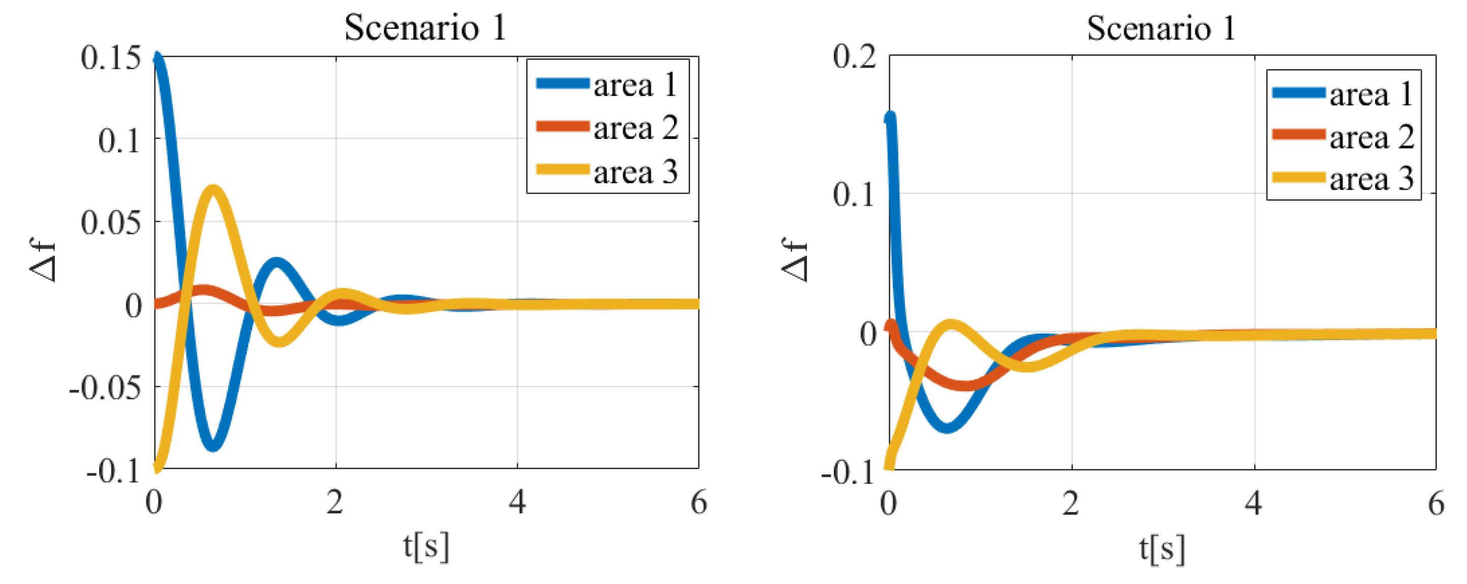
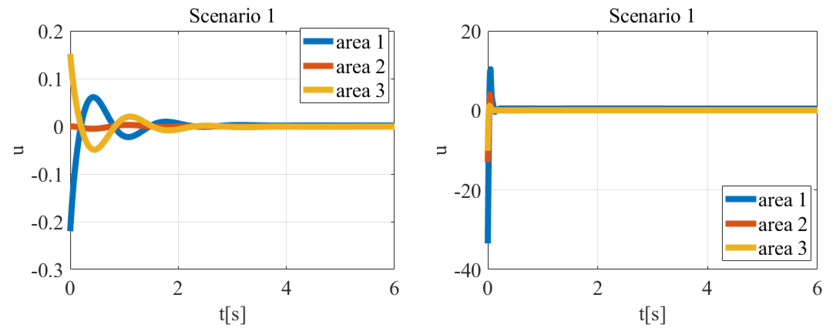
In the first simulation scenario, the system responded to the non-zero initial conditions. In the case of the LQR control strategy, areas 1 and 3 had similar quality indices, while area 2 had the smallest maximum errors, and area 3 had the biggest overshoot. The energy generated by the controller was biggest in area 1 and smallest in area 2 (ISV index). In the case of the FLC control strategy, the quality indexes, and energy generated by the controller, were similar for all areas. In terms of integral indexes (IAE, ITAE, ISV), the LFC control strategy was worse than the LQR strategy—the biggest difference was in case of area 1. Furthermore, in all areas there was visible large overshoot.

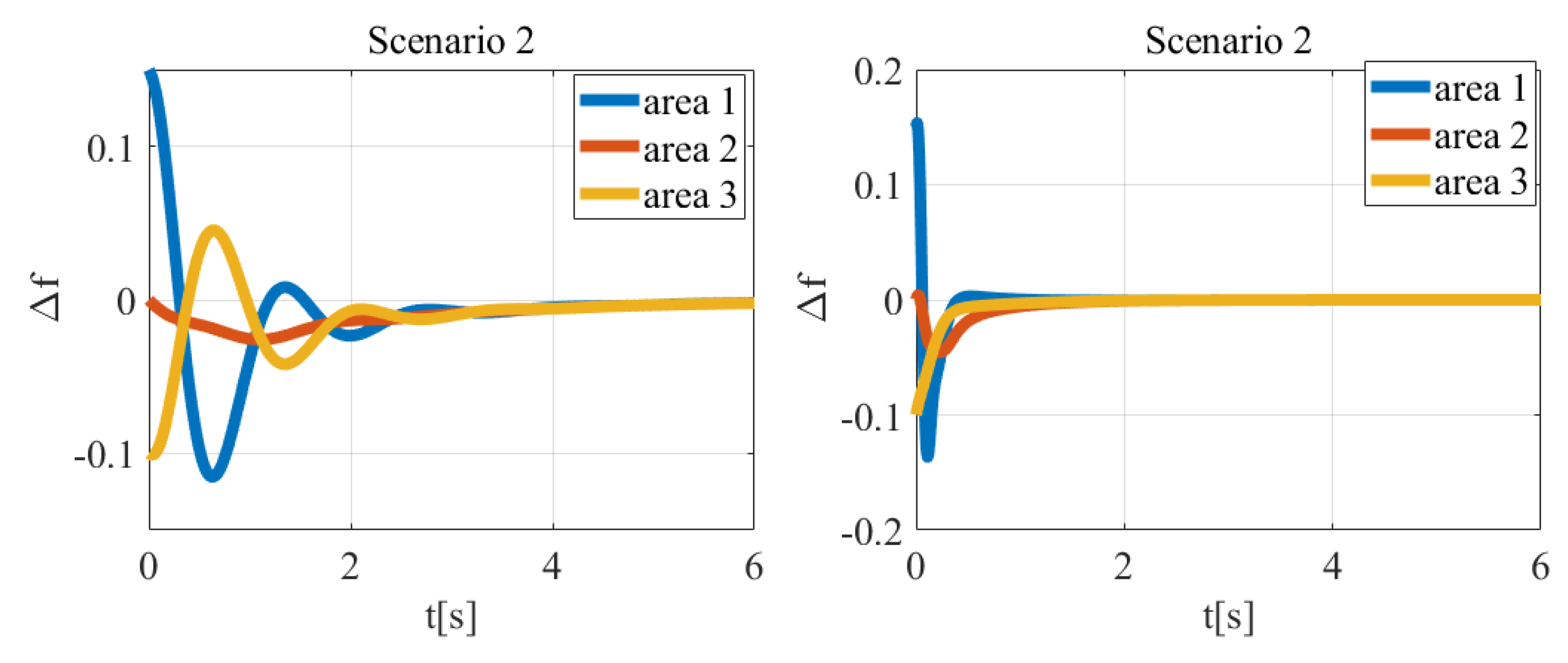
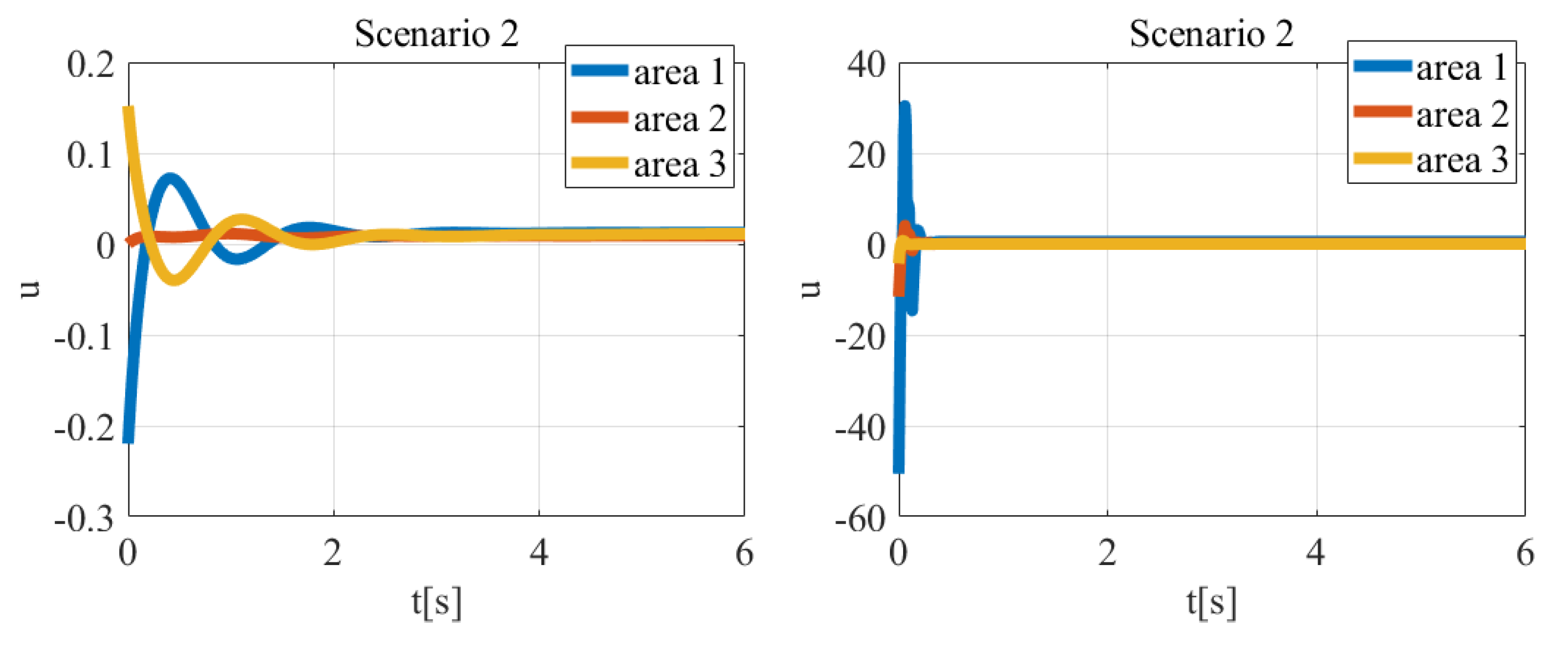
In the second simulation scenario, the system responded to the step-change in the disturbance load. It measures the robustness of the control system to external interferences. In the case of the LQR control strategy, it’s visible that area 2 have a small overshoot, comparing to area 1 and area 3. The energy generated by the controller was biggest in area 3 and smallest in area 1 (ISV index). In the case of the FLC control strategy the quality indexes, and energy generated by the controller, were similar for all areas. In terms of integral indexes (IAE, ITAE), the LFC control strategy was slightly better than the LQR strategy, with significantly worse energy consumption. Furthermore, in all areas there was visible large overshoot.

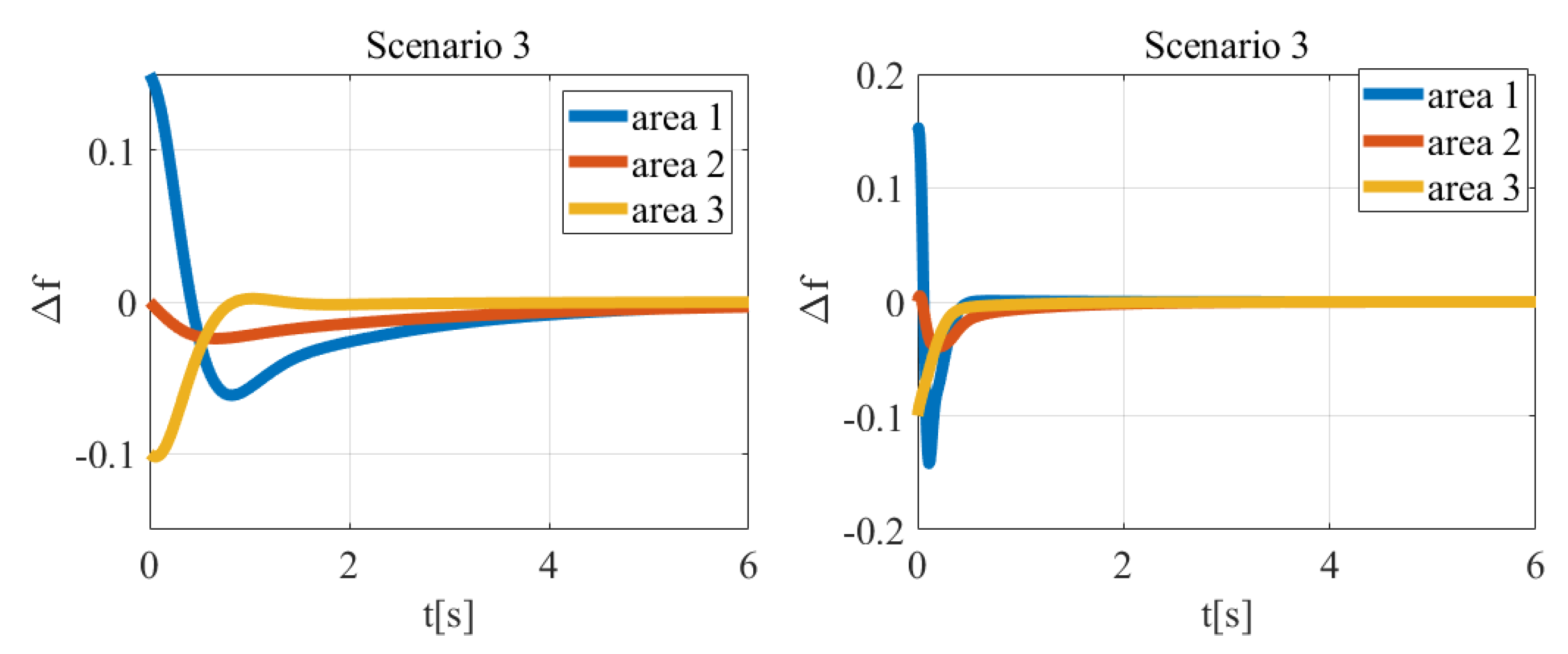
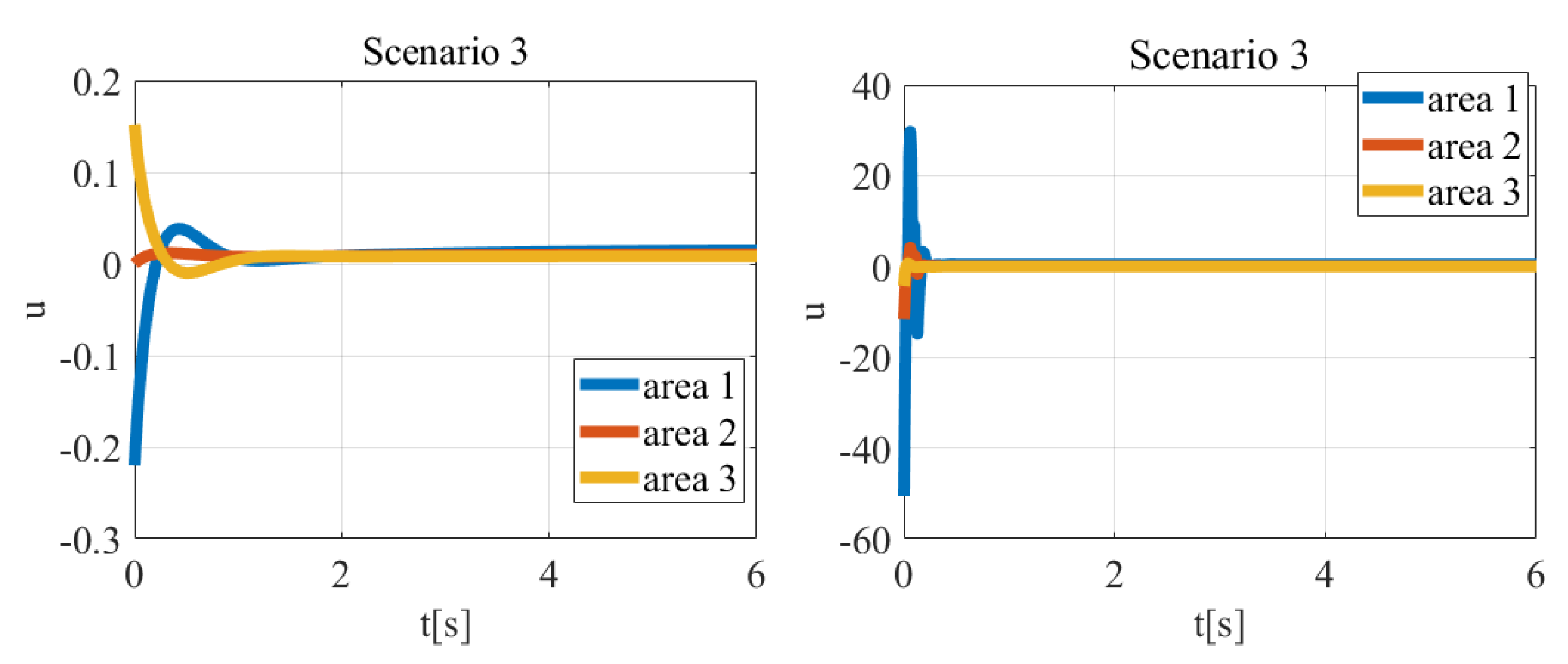
In the final third simulation scenario, the areas in the system were fully decouples, with all areas working independently. This, comparing with scenario 1 and 2, allowed us to add progressively the faults in the system, and thus check the robustness. In the case of the LQR control strategy, area 1 had the worst performance and energy consumption, while area 2 had the best performance and energy consumption. The performance in area 3 is rather in between other areas. In the case of the FLC control strategy, the performance measures were similar for all areas. However, in terms of integral indexes (IAE, ITAE), the LFC control strategy was better than the LQR strategy, but it was worse in terms of the energy consumption.

The obtained results show the significant differences in the performance of the presented control methods of the three-area power generation system. The performance of the LQR control strategy is better than the performance of the FLC strategy, in terms of most calculated quality indexes and energy consumption. Note that the LQR control is a model-based strategy, and it is strongly dependent on the quality of the provided model and requires the model in the linear form. The advantage is rather simple method to calculate the controller gains. On the contrary, the FLC control system is much easier to implement and develop, as it is a data-driven expert-based methodology.

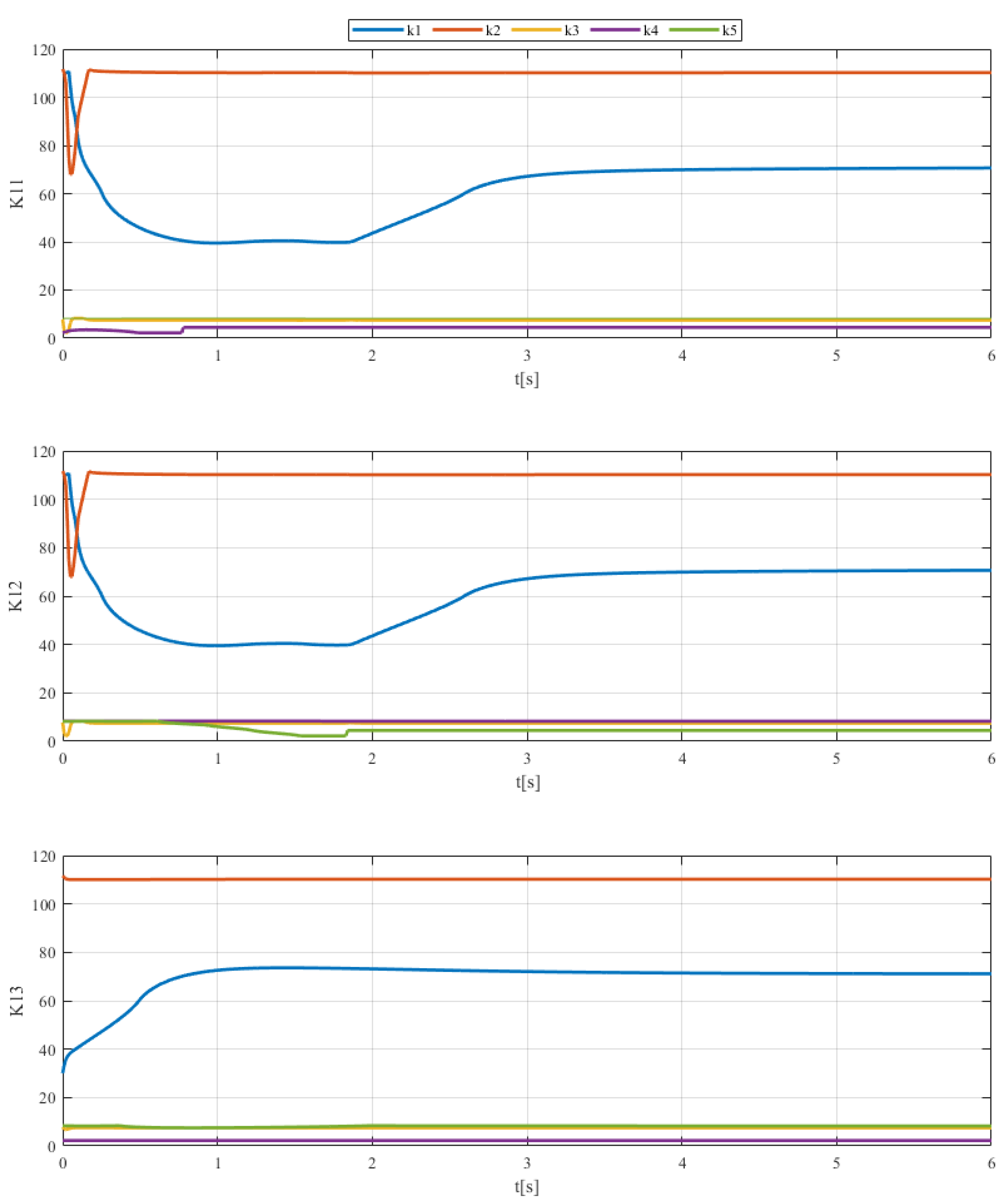
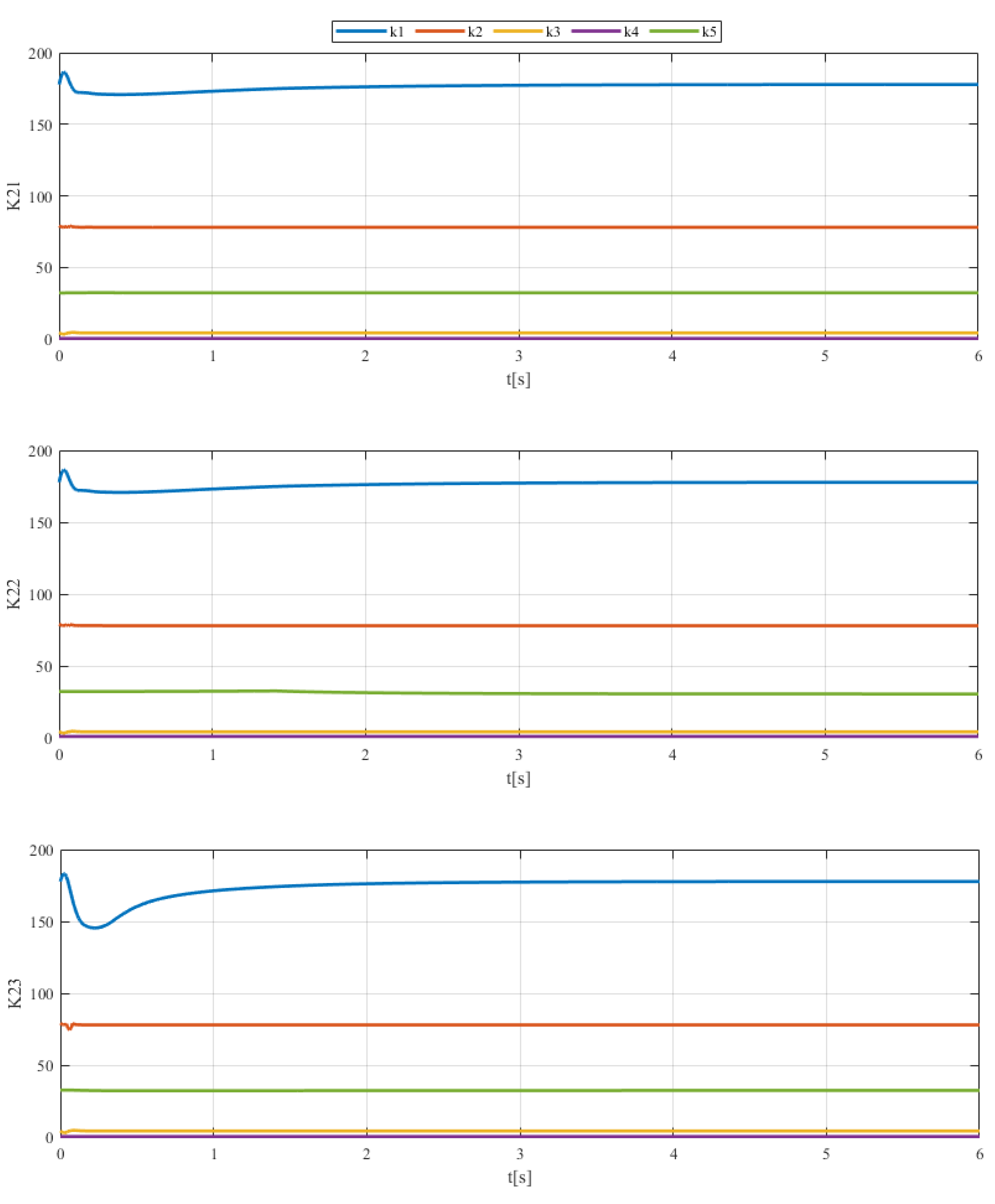
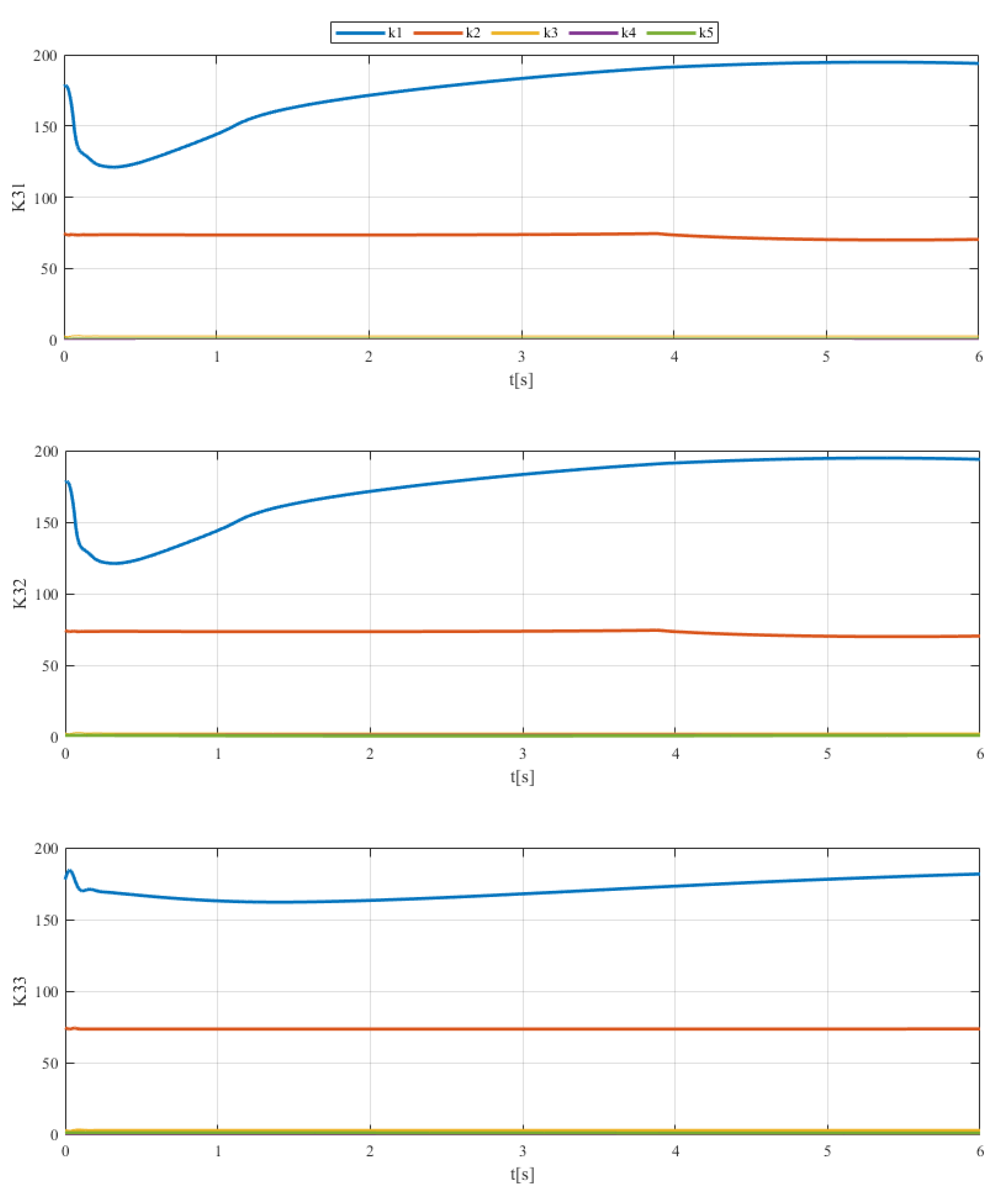
The differences in the performance and energy consumption can be explained by the significant differences in the controller gains between LQR and FLC algorithms (see Table 3, Table 4 and Table 5, and Figure 7, Figure 8 and Figure 9). The gains values and their range of changes during adaptation of FLC controller are much higher than the optimal values of the LQR controller. Thus, we get a very strong control signal.

However, the LQR controller have significant drawbacks. It is model-based optimal controller, and it requires the exact model in the state-space linear form. It does not preserve robustness from parameter changes and external disturbances characterizing real-life systems [60]. In contrary, the FLC controller is fully data-driven, and the model is in form of cause–effect relationship functions, derived on the basis of the expert knowledge. Fuzzy control system can be used especially for the complex nonlinear process that includes uncertainty, and therefore there is no precise mathematical model available [61] that, to some extent, can overcome the above-mentioned problems of LQR control system.

The biggest challenge, in case of FLC, is the definition of the rule base, and the controller parameters tuning. Most of the FLC controller tuning methods are based on genetic algorithms [62], particle swarm optimization [63] and therefore are time-consuming and very hard for practical implementation.

Therefore, the very simple method to minimize the gains is the introduction of the constraints of the gains.

5. Conclusions

This paper presents the comparison of two different strategies of the three-area power generation system (micro-grid) control. The first one is a model-based Linear Quadratic Regulator (LQR) strategy, where one optimal controller generates the control signal for all three areas. The second one is a data-driven Fuzzy Logic Controller (FLC), distributed to three areas, i.e., there is one FLC controller for each area.

The comparison was made, based on three scenarios describing different working conditions of the system, with the changing load, and decoupling of the areas. Both controllers worked properly in all scenarios; however, as the provided values of the calculated quality indexes show, the FLC control strategy is worse than the LQR strategy. It is mostly due to the difficult methodology of the FLC controller tuning. We can conclude that even if the data-driven methods do not require the model of the system and stabilize the system as expected, there are still problems with the proper choice of their parameters to obtain the desired performance.

The results obtained during the presented research, with the three area power generation system, showed that to apply the proposed control algorithms it is crucial to develop methods for tuning the controllers, especially the data-driven ones, to minimize the influence of disturbances and changes of the parameters. The proposed future work includes research on tuning methods of FLC controllers, and the comparison of the performance of the distributed control strategy in case of failures in areas (e.g., as the result of the cyber-attack).

References

1. Bevrani, H.; Habibi, F.; Babahajyani, P.; Watanabe, M.; Mitani, Y. Intelligent frequency control in an AC microgrid: Online PSO-based fuzzy tuning approach. IEEE Trans. Smart Grid 2012, 3, 1935–1944. [Google Scholar] [CrossRef]
2. Zribi, M.; Al-Rashed, M.; Alrifai, M. Adaptive decentralized load frequency control of multi-area power systems. Int. J. Electr. Power Energy Syst. 2005, 27, 575–583. [Google Scholar] [CrossRef]
3. AlRifai, M.; Zribi, M. A robust decentralized controller for power system load frequency control. In Proceedings of the 39th International Universities Power Engineering Conference—UPEC 2004, Bristol, UK, 6–8 September 2004; Volume 2, pp. 794–799. [Google Scholar]
4. Malik, O.; Kumar, A.; Hope, G. A load frequency control algorithm based on a generalized approach. IEEE Trans. Power Syst. 1988, 3, 375–382. [Google Scholar] [CrossRef]
5. Bevrani, H.; Hiyama, T. Intelligent Automatic Generation Control; CRC Press: Boca Raton, FL, USA, 2011. [Google Scholar] [CrossRef]
6. De Silva, C.W. Intelligent Control: Fuzzy Logic Applications; CRC Press: Boca Raton, FL, USA, 1995. [Google Scholar] [CrossRef]
7. Yao, E.; Wong, V.W.; Schober, R. Robust frequency regulation capacity scheduling algorithm for electric vehicles. IEEE Trans. Smart Grid 2016, 8, 984–997. [Google Scholar] [CrossRef]
8. Ma, M.; Zhang, C.; Liu, X.; Chen, H. Distributed model predictive load frequency control of the multi-area power system after deregulation. IEEE Trans. Ind. Electron. 2016, 64, 5129–5139. [Google Scholar] [CrossRef]
9. Cominesi, S.R.; Farina, M.; Giulioni, L.; Picasso, B.; Scattolini, R. A two-layer stochastic model predictive control scheme for microgrids. IEEE Trans. Control Syst. Technol. 2017, 26, 1–13. [Google Scholar] [CrossRef]
10. Xu, Y.; Li, F.; Jin, Z.; Variani, M.H. Dynamic gain-tuning control (DGTC) approach for AGC with effects of wind power. IEEE Trans. Power Syst. 2015, 31, 3339–3348. [Google Scholar] [CrossRef]
11. Chen, X.; Lin, J.; Liu, F.; Song, Y. Optimal control of AGC systems considering non-gaussian wind power uncertainty. IEEE Trans. Power Syst. 2019, 34, 2730–2743. [Google Scholar] [CrossRef] [Green Version]
12. Liu, X.; Zhang, Y.; Lee, K.Y. Coordinated distributed MPC for load frequency control of power system with wind farms. IEEE Trans. Ind. Electron. 2016, 64, 5140–5150. [Google Scholar] [CrossRef]
13. Kumar, L.S.; Kumar, G.N.; Madichetty, S. Pattern search algorithm based automatic online parameter estimation for AGC with effects of wind power. Int. J. Electr. Power Energy Syst. 2017, 84, 135–142. [Google Scholar] [CrossRef]
14. Abd-Elazim, S.; Ali, E. Load frequency controller design of a two-area system composing of PV grid and thermal generator via firefly algorithm. Neural Comput. Appl. 2018, 30, 607–616. [Google Scholar] [CrossRef]
15. Zeng, G.-Q.; Xie, X.-Q.; Chen, M.-R. An adaptive model predictive load frequency control method for multi-area interconnected power systems with photovoltaic generations. Energies 2017, 10, 1840. [Google Scholar] [CrossRef] [Green Version]
16. Bevrani, H.; Daneshmand, P.R. Fuzzy logic-based load-frequency control concerning high penetration of wind turbines. IEEE Syst. J. 2011, 6, 173–180. [Google Scholar] [CrossRef]
17. Sahu, R.K.; Panda, S.; Rout, U.K. DE optimized parallel 2-DOF PID controller for load frequency control of power system with governor dead-band nonlinearity. Int. J. Electr. Power Energy Syst. 2013, 49, 19–33. [Google Scholar] [CrossRef]
18. Fathy, A.; Kassem, A.M.; Abdelaziz, A.Y. Optimal design of fuzzy PID controller for deregulated LFC of multi-area power system via mine blast algorithm. Neural Comput. Appl. 2020, 32, 4531–4551. [Google Scholar] [CrossRef]
19. Nosratabadi, S.M.; Bornapour, M.; Gharaei, M.A. Grasshopper optimization algorithm for optimal load frequency control considering predictive functional modified PID controller in restructured multi-resource multi-area power system with redox flow battery units. Control Eng. Pract. 2019, 89, 204–227. [Google Scholar] [CrossRef]
20. Saxena, S.; Hote, Y.V. Decentralized PID load frequency control for perturbed multi-area power systems. Int. J. Electr. Power Energy Syst. 2016, 81, 405–415. [Google Scholar] [CrossRef]
21. Tan, W. Unified tuning of PID load frequency controller for power systems via IMC. IEEE Trans. Power Syst. 2009, 25, 341–350. [Google Scholar] [CrossRef]
22. Yang, D.; Wang, B.; Cai, G.; Ma, J.; Tian, J.; Chen, Z.; Wang, L. Inertia-adaptive model predictive control-based load frequency control for interconnected power systems with wind power. IET Gener. Transm. Distrib. 2020, 14, 5029–5036. [Google Scholar] [CrossRef]
23. Yang, J.; Sun, X.; Liao, K.; He, Z.; Cai, L. Model predictive control-based load frequency control for power systems with wind-turbine generators. IET Renew. Power Gener. 2019, 13, 2871–2879. [Google Scholar] [CrossRef]
24. Oshnoei, A.; Kheradmandi, M.; Khezri, R.; Mahmoudi, A. Robust Model Predictive Control of Gate-Controlled Series Capacitor for LFC of Power Systems. IEEE Trans. Ind. Inform. 2021, 17, 4766–4776. [Google Scholar] [CrossRef]
25. Chuang, N. Robust H load-frequency control in interconnected power systems. IET Control Theory Appl. 2016, 10, 67–75. [Google Scholar] [CrossRef]
26. Sabahi, K.; Teshnehlab, M. Recurrent fuzzy neural network by using feedback error learning approaches for LFC in interconnected power system. Energy Convers. Manag. 2009, 50, 938–946. [Google Scholar] [CrossRef]
27. Lv, X.; Sun, Y.; Cao, S.; Dinavahi, V. Event-triggered load frequency control for multi-area power systems based on Markov model: A global sliding mode control approach. IET Gener. Transm. Distrib. 2020, 14, 4878–4887. [Google Scholar] [CrossRef]
28. Lv, X.; Sun, Y.; Wang, Y.; Dinavahi, V. Adaptive event-triggered load frequency control of multi-area power systems under networked environment via sliding mode control. IEEE Access 2020, 8, 86585–86594. [Google Scholar] [CrossRef]
29. Prasad, S.; Purwar, S.; Kishor, N. Non-linear sliding mode load frequency control in multi-area power system. Control Eng. Pract. 2017, 61, 81–92. [Google Scholar] [CrossRef]
30. Karimi, A.; Feliachi, A. Decentralized adaptive backstepping control of electric power systems. Electr. Power Syst. Res. 2008, 78, 484–493. [Google Scholar] [CrossRef]
31. Gao, W.; Wang, Y.; Homaifa, A. Discrete-time variable structure control systems. IEEE Trans. Ind. Electron. 1995, 42, 117–122. [Google Scholar] [CrossRef]
32. Mi, Y.; Fu, Y.; Li, D.; Wang, C.; Loh, P.C.; Wang, P. The sliding mode load frequency control for hybrid power system based on disturbance observer. Int. J. Electr. Power Energy Syst. 2016, 74, 446–452. [Google Scholar] [CrossRef]
33. Hosseinabadi, P.A.; Abadi, A.S.S.; Mekhilef, S.; Pota, H.R. Fixed-time adaptive robust synchronization with a state observer of chaotic support structures for offshore wind turbines. J. Control Autom. Electr. Syst. 2021, 32, 942–955. [Google Scholar] [CrossRef]
34. Khodabakhshian, A.; Edrisi, M. A new robust PID load frequency controller. Control Eng. Pract. 2008, 16, 1069–1080. [Google Scholar] [CrossRef]
35. Prepared by NERC RS Committee. Balancing and Frequency Control: A Technical Document Prepared by the NERC Resources Subcommittee. NERC Technical Report. 2011. Available online: https://www.coursehero.com/file/6329489/NERC-Balancing-and-Frequency-Control-July-5-2009/ (accessed on 26 January 2011).
36. Aditya, S.; Das, D. Load-frequency control of an interconnected hydro-thermal power system with new area control error considering battery energy storage facility. Int. J. Energy Res. 2000, 24, 525–538. [Google Scholar] [CrossRef]
37. Polajžer, B.; Petrun, M.; Ritonja, J. Adaptation of load-frequency-control target values based on the covariances between area-control errors. IEEE Trans. Power Syst. 2018, 33, 5865–5874. [Google Scholar] [CrossRef]
38. Das, D.; Gurrala, G.; Shenoy, U.J. Linear quadratic regulator-based bumpless transfer in microgrids. IEEE Trans. Smart Grid 2016, 9, 416–425. [Google Scholar] [CrossRef]
39. Pradeep, K.; Mouli, C.C.; Reddy, K.S.P.; Raju, K.N. Design and development of optimal controller for photovoltaic system. Int. J. Adv. Sci. Technol. Res. 2015, 1, 377–383. [Google Scholar]
40. Yu, B.; Zhang, Y.; Minchala, I.; Qu, Y. Fault-tolerant control with linear quadratic and model predictive control techniques against actuator faults in a quadrotor UAV. In Proceedings of the 2013 Conference on Control and Fault-Tolerant Systems (SysTol), Nice, France, 9–11 October 2013; pp. 661–666. [Google Scholar] [CrossRef]
41. Jorge Miguel Brito Domingues, Quadrotor Prototype, Instituto Superior Técnico, Portugal. 5 October 2009. Available online: https://www.docsity.com/pt/quadrotor-prototype-msc-jorge-m-b-domingues/4767460/ (accessed on 29 November 2021).
42. Bouzid, A.M.; Guerrero, J.M.; Cheriti, A.; Bouhamida, M.; Sicard, P.; Benghanem, M. A survey on control of electric power distributed generation systems for microgrid applications. Renew. Sustain. Energy Rev. 2015, 44, 751–766. [Google Scholar] [CrossRef] [Green Version]
43. Karanjkar, D.; Chatterji, S.; Kumar, A. Design and implementation of a linear quadratic regulator based maximum power point tracker for solar photo-voltaic system. Int. J. Hybrid Inf. Technol. 2014, 7, 167–182. [Google Scholar] [CrossRef]
44. Vandoorn, T.L.; Renders, B.; Degroote, L.; Meersman, B.; Vandevelde, L. Voltage control in islanded microgrids by means of a linear-quadratic regulator. In Proceedings of the IEEE Benelux Young Researchers Symposium in Electrical Power Engineering (YRS’10), Leuven, Belgium, 29 March 2010. [Google Scholar]
45. Pourmousavi, S.A.; Nehrir, M.H. Introducing dynamic demand response in the LFC model. IEEE Trans. Power Syst. 2014, 29, 1562–1572. [Google Scholar] [CrossRef]
46. Devi, P.S.; Santhi, R.V.; Pushpalatha, D. Introducing LQR-fuzzy technique with dynamic demand response control loop to load frequency control model. IFAC-PapersOnLine 2016, 49, 567–572. [Google Scholar] [CrossRef]
47. Camci, E.; Kripalani, D.R.; Ma, L.; Kayacan, E.; Khanesar, M.A. An aerial robot for rice farm quality inspection with type-2 fuzzy neural networks tuned by particle swarm optimization-sliding mode control hybrid algorithm. Swarm Evol. Comput. 2017, 41, 1–8. [Google Scholar] [CrossRef] [Green Version]
48. Yin, S.; Shi, P.; Yang, H. Adaptive fuzzy control of strict-feedback nonlinear time-delay systems with unmodeled dynamics. IEEE Trans. Cybern. 2016, 46, 1926–1938. [Google Scholar] [CrossRef]
49. Cheong, F. A hierarchical fuzzy system with high input dimensions for forecasting foreign exchange rates. In Proceedings of the 2007 IEEE Congress on Evolutionary Computation, Singapore, 25–28 September 2007. [Google Scholar] [CrossRef] [Green Version]
50. Khadija, E.H.; Abdeljalil, E.K.; Mostafa, M.; Hassan, A. Adapting parameters for flight control of a quadcopter using reference model and fuzzy logic. In Proceedings of the 2015 Third World Conference on Complex Systems (WCCS), Marrakech, Morocco, 23–25 November 2015; pp. 1–6. [Google Scholar] [CrossRef]
51. Abadi, A.S.S.; Hosseinabadi, P.A.; Mekhilef, S. Fuzzy adaptive fixed-time sliding mode control with state observer for a class of high-order mismatched uncertain systems. Int. J. Control Autom. Syst. 2020, 18, 2492–2508. [Google Scholar] [CrossRef]
52. Yang, Y.; Yan, Y. Attitude regulation for unmanned quadrotors using adaptive fuzzy gain-scheduling sliding mode control. Aerosp. Sci. Technol. 2016, 54, 208–217. [Google Scholar] [CrossRef]
53. Sibilska-Mroziewicz, A. Model of Multi-Area Power System. MATLAB Central File Exchange. 2021. Available online: https://www.mathworks.com/matlabcentral/fileexchange/102714-model-of-multi-area-power-system (accessed on 29 November 2021).
54. Yousef, H.A.; Khalfan, A.-K.; Albadi, M.H.; Hosseinzadeh, N. Load frequency control of a multi-area power system: An adaptive fuzzy logic approach. IEEE Trans. Power Syst. 2014, 29, 1822–1830. [Google Scholar] [CrossRef]
55. Chen, Y.-K.; Wu, Y.-C.; Song, C.-C.; Chen, Y.-S. Design and implementation of energy management system with fuzzy control for DC microgrid systems. IEEE Trans. Power Electron. 2013, 28, 1563–1570. [Google Scholar] [CrossRef]
56. Ahmadi, S.; Shokoohi, S.; Bevrani, H. A fuzzy logic-based droop control for simultaneous voltage and frequency regulation in an AC microgrid. Int. J. Electr. Power Energy Syst. 2015, 64, 148–155. [Google Scholar] [CrossRef]
57. Bryson, A.E.; Ho, Y.-C. Applied Optimal Control Optimization, Estimation and Control; CRC Press: Boca Raton, FL, USA, 1975. [Google Scholar] [CrossRef]
58. Mozaryn, J.; Malinowski, K. Tuning rules selection and iterative modification of PID control system parameters. In Mechatronics 2013; Brezina, T., Jablonski, R., Eds.; Springer: Cham, Switzerland, 2013. [Google Scholar] [CrossRef]
59. Alinaghi Hosseinabadi, P.; Ordys, A.; Soltani Sharif Abadi, A.; Mekhilef, S.; Pota, H.R. State and disturbance observers-based chattering-free fixed-time sliding mode control for a class of high-order nonlinear systems. Adv. Control Appl. Eng. Ind. Syst. 2021, 3, e81. [Google Scholar] [CrossRef]
60. Liu, X.; Wu, Y.; Zhang, Y.; Xiao, S. Control Method to Make LQR Robust: A Planes Cluster Approaching Mode. Int. J. Control Autom. Syst. 2014, 12, 302–308. [Google Scholar] [CrossRef]
61. Kluska, J. Analytical Methods in Fuzzy Modeling and Control; Studies in Fuzziness and Soft Computing; Springer: Berlin/Heidelberg, Germeny, 2019; Volume 241. [Google Scholar] [CrossRef]
62. Herrera, F.; Lozano, M.; Verdegay, J.L. Tuning fuzzy logic controllers by genetic algorithms. Int. J. Approx. Reason. 1995, 12, 299–315. [Google Scholar] [CrossRef] [Green Version]
63. Faisal, M.; Hannan, M.A.; Ker, P.J.; Rahman, M.A.; Begum, R.A.; Mahlia, T.M.I. Particle swarm optimised fuzzy controller for charging–discharging and scheduling of battery energy storage system in MG applications. Energy Rep. 2020, 6, 215–228. [Google Scholar] [CrossRef]
Figure 1. i-tharea model of the N-area power system.
Energies 14 08522 g001
Figure 2. The block diagram of the control of three-area power generation system.
Energies 14 08522 g002
Figure 3. The structure of fuzzy system.
Energies 14 08522 g003
Figure 4. Input membership function Scenarios 1, 2, and 3.
Energies 14 08522 g004
Figure 5. Output membership function for Scenario 1.
Energies 14 08522 g005
Figure 6. Output membership function for Scenarios 2 and 3.
Energies 14 08522 g006
Figure 7. Controller gains of FLC for K11 (scenario 1, area 1), K12 (scenario 1, area 2), and K13 (scenario 1, area 3).
Energies 14 08522 g007
Figure 8. Controller gains of FLC for K21 (scenario 2, area 1), K22 (scenario 2, area 2), and K23 (scenario 2, area 3).
Energies 14 08522 g008
Figure 9. Controller gains of FLC for K31 (scenario 3, area 1), K32 (scenario 3, area 2), and K33 (scenario 3, area 3).
Energies 14 08522 g009
Figure 10. The time responses of Δ f with LQR (left figure) and fuzzy controller (right figure) for different areas—scenario 1.
Energies 14 08522 g010
Figure 11. Control signals u ( t ) with LQR (left figure) and fuzzy controller (right figure) for different areas—scenario 1.
Energies 14 08522 g011
Figure 12. The time responses of Δ f with LQR (left figure) and fuzzy controller (right figure) for different areas—scenario 2.
Energies 14 08522 g012
Figure 13. Control signals u ( t ) with LQR (left figure) and fuzzy controller (right figure) for different areas—scenario 2.
Energies 14 08522 g013
Figure 14. The time responses of Δ f with LQR (left figure) and fuzzy controller (right figure) controller for different areas—scenario 3.
Energies 14 08522 g014
Figure 15. Control signals u ( t ) with LQR (left figure) and fuzzy controller (right figure) for different areas—scenario 3.
Energies 14 08522 g015