Article

Scenarios Analysis on Electric Power Planning Based on Multi-Scale Forecast: A Case Study of Taoussa, Mali from 2020 to 2035

1
Key Laboratory of Efficient Utilization of Low and Medium Grade Energy, Tianjin University, MOE, Tianjin 300350, China
2
Department of Electrical Engineering, Vocational School of Soumangourou KANTÉ, University of Bamako, Bamako 63, Mali
*
Author to whom correspondence should be addressed.
Energies 2021, 14(24), 8515; https://doi.org/10.3390/en14248515
Submission received: 8 October 2021 / Revised: 7 November 2021 / Accepted: 9 December 2021 / Published: 17 December 2021
(This article belongs to the Topic Electricity Demand-Side Management)

Abstract

:
The increase in electricity demand is caused by population density, gross domestic product growth and technological conditions. A long-term forecast study on the electricity demand could be a promising alternative to the investment planning of power systems and distribution. In this study, the main aim is to forecast and understand the long-term electricity demand of the Taoussa area for the sustainable development of the regions of northern Mali, by using the Model for Analysis of Energy Demand (MAED) from the International Atomic Energy Agency. To fill such a knowledge gap, the long-term evolution of electricity demand is calculated separately for four consumption sectors: industry, transportation, service and household from 2020 to 2035. The demand for each end-use category of electricity is driven by one or several socioeconomic and technological parameters development of the country, which are given as part of the reference scenario (RS) and two alternative scenarios (Low and High). These scenarios were developed based on four groups of coherent hypotheses concerning demographic evolution, economic development, lifestyle change and technological change. The results showed that the annual growth rate of electricity demand in Taoussa area in all scenarios is expected to increase by only 8.13% (LS), 10.31% (RS) and 12.56% (HS). According to the seasonal variations of electricity demand, dry season electricity demand was higher than the demand in cool season during the study period. Such a conclusion demonstrates that the proposed long-term method and related results could provide powerful sustainable solutions to the electricity development challenges of Africa.

Graphical Abstract

1. Introduction

Energy is essential for economic and social development and improved quality of life. However, much of the world’s energy is currently produced and used in ways that may not be sustainable in the long term. In order to assess progress towards a sustainable energy future (solar energy, wind energy, tidal energy and geothermal energy), energy indicators that can measure and monitor important changes are needed [1].
Energy demand is a derived demand that arises to satisfy some needs which are met through the use of appliances. Hence, demand for energy then depends on the demand for energy services and the choice of energy using processes or devices. End-use service demand is affected by the cost of energy but also by other factors such as climatic conditions, affordability (or income of the decision-maker), preference for the end-use service, etc. Similarly, demand for end-use appliances depends on the relative prices of the appliances, relative cost of operation, availability of appliances, etc. [2]. The expected future trends for these determining factors, which constitute ‘scenarios’, are exogenously introduced. The scenario is a potential image whose future could be revealed; a set of scenarios helps to understand the possible future evolutions of complex systems. For example, a scenario can consider in the long term a series of future socio-economic and technical data (population growth rate, GDP growth rate, structural changes in the economy, improvement of household size, improvement of efficiency) to examine energy demand [3].
A model for peak-load demand should take into account the following factors or part of them, depending on the country in which this model is going to be implemented. There is no unique model that can be applied to utility companies.
These factors are
The gross domestic product (GDP)
The population (POP)
The GDP per capita (GDP/CAP)
The multiplication of electricity consumption by population (EP)
The power system losses (LOSS)
The load factor (LF)
The cost of one kilowatt hour (the average rate per unit sale; R/S) (mill/kWh).
The first four factors depend on the behavior of the public; thus, they may vary from country to country, whereas the last three factors depend on the electric power system and the load itself, as well as the consumption of power generated [4].
Electricity load forecasting is a multifaceted task that encompasses various sides of the economical and safety operations of power supply systems. The forecasting provides assistance for security analysis of supply systems, system control, maintenance, etc. It also provides feedback for planning. By considering these important facets of the forecasting, many methods have been applied to predict electricity load forecasting over years to get more accurate results for efficient planning, however, the prediction has still remained a challenging issue that contains many uncertain factors affecting electricity load utilization [5].
There are mostly three categories of energy consumption studies in the literature according to the forecasting horizon. Long-term forecasting (5 to 20 years) is mostly applied for resource management and development investments. Mid-term forecasting (a month to five years) is mostly applied for planning the power production resources and tariffs, and short-term forecasting (an hour to a week) is mostly used for scheduling and analyses of the distribution network [6].
Each one of these planning horizons is important; however, long-term forecasting can be considered the most critical horizon due to the consequences of the strategic and costly decisions, such as the expansion of utility plants. An overestimation of electricity demand, especially in long-term forecasting, will result in a significant increase in the construction of unnecessary electricity generation plants. In contrast, an underestimation of electricity demand forecasting will result in a shortage of electricity production and customer dissatisfaction [7].
It is not surprising that factors affecting prediction horizon types may vary. In the short-term and mid-term load forecasting, the most important factor for load prediction is the complexity of an economy and a weather factor of the whole area, however, in long-term load forecasting, GDP, expected economic situations, changes in the demography, etc. are the most common factors which affect load usage [8,9].
The forecasting methods are classified into traditional (e.g., fuzzy logic, grey model, metaheuristic algorithms, regression models, simulation model, time series model) and intelligent (e.g., machine learning and neural network) models. Furthermore, the advantages and disadvantages of both traditional and intelligent forecasting methods as well as research limitations and future research have been determined [10]. The historic time series data are used in many studies to predict energy consumption, the effect of variables such as GDP, consumer price index (CPI), humidity, temperature, population, energy price, daylight time, number of rainy days, etc. on energy consumption is analyzed in many others. Proposed models can be applied by the producers, suppliers and regulatory authorities who want to securely supply the electricity at a reasonable cost [11].
Researchers use different models and methodologies to forecast electricity demand. For example, the work in [12] used a hybrid load-forecasting method that combines classical time series formulations with cubic splines to model electricity load; only the hourly temperature is used in the proposed model and predictive power gains are achieved through the modeling of the 24-h load profiles across weekends and weekdays while also taking into consideration seasonal variations of such profiles. Long-term trends are accounted for by using population and economic variables. The authors of [13] proposed a deep residual neural network model for day-ahead household electrical energy consumption forecasting and integrated multiple sources of information (weather, calendar and historical load). In [14], the authors employed a fuzzy logic model for long-term load forecasting for one year based on the weather parameters (temperature and humidity) and historical load data. The work in [7] presented long-term forecasting of electrical loads in Kuwait using Prophet and Holt-Winters models for ten years based on the real data of historical electric load peaks. The authors of [15] also designed enhanced machine learning techniques for electricity load and price forecasting, and hourly data of one year are used for the forecasting process. In [16], the author developed a scenario-based model for the African power system using the Schwartz methodology. The work in [17] showed the superiority of triple seasonal methods of Holt-Winters and autoregressive moving average (ARMA) models for short-term electricity demand forecasting.
Many future electricity demand projection studies in the literature research have employed a bottom-up approach using the Model for Analysis of Energy Demand—Energy Demand module (MAED_D), which adopts socio-economic and technological development indicators to make long-term projections in the case of Syria, Turkey, Nigeria, Nepal, Tanzania, Bangladesh and Lesotho.
The final energy demand and the final electricity demand of Syria will grow annually. Both final energy and electricity demand growth rates are lower than the corresponding GDP growth rates, which indicate positive development trends in the elasticity evolution. However, the growth of electricity is continuously higher than that of final energy with increasing tendency over the whole study period. This is a direct result of more automation in industry and more electrical equipment in households and services [18]. The MAED model was executed for the above three scenarios and Turkey’s annual electric energy demand values were predicted from the study period. The result shows that the future electricity demand will be growing rapidly in Turkey [19]. The forecast of the energy demand of Tanzania for all economic sectors was analyzed by using the Model for Analysis of Energy Demand (MAED) for the study period. In the study, three scenarios were formulated to simulate possible future long-term energy demand based on socio-economic and technological development with the base year. The study results show that the highest growth rate of electricity demand is in the industry sector, followed closely by the service and household sectors [20].
The second module of MAED, MAED_EL (EL = electricity) was used to determine the annual peak load of future Syrian electric power demand. The results indicate that the current residential behavior of the Syrian power system will shift in the reference scenario more and more to the typical industry behavior characterized by higher load factors. The future peak load will grow annually [21].
The major contribution of the work in this paper is to improve estimates of future electrical energy needs of Taoussa using the Model for Analysis of Energy Demand (MAED) on the long-term evolution of electricity demand for the sustainable development of the regions of northern Mali. National economic and energy statistics provide the input to the calibration of the model to accurately reflect the current electricity system as well as its interaction with the principal drivers of electricity demand, such as demographics, economic development, technological change, environmental policy, etc. Energy planners can then compare these scenarios (different futures) with their ability to support national development objectives and goals. Critical policy and investment aspects of different energy strategies can be defined, undesirable consequences can be identified, and the most cost-effective approach to meeting future electricity needs can be determined.
The rest of this article is organized as follows. 
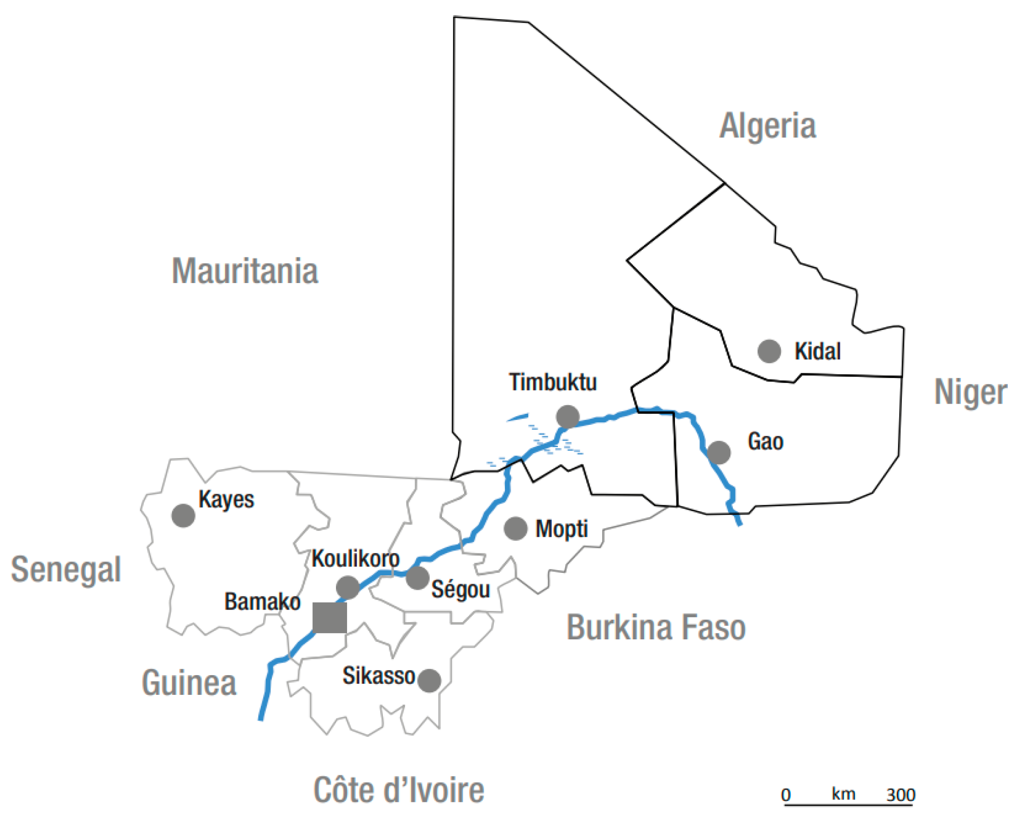
Section 2 presents general information on the case study. Section 3 talks about the IAEA’s tools and models. Section 4 describes scenarios and background information employed in the MAED model. Section 5 predicts the electricity demand under three scenarios and indicates future research directions, and finally, conclusions are elaborated in Section 6.

2. Information on the Taoussa Area

Mali is one of the landlocked countries of the Sahelian and half of the national territory is located in the Saharan zone of West Africa, as shown in Figure 1.
Its surface area is 1,241,248 km2; 60% of it is desert land (north). It is located between 10° and 25° north in latitude, 3° east and 12° west in longitude. Two of the most important rivers in West Africa cross it; these are the Niger River and Senegal River.
The Taoussa area in Mali is located in the northern regions (Timbuktu and Gao), it has a Sahelian to sub-Saharan climate, and is characterized by low rainfall and limited water resources which generates a strong dependence on water and energy. In response to the worrying situation in the northern regions, the government of Mali is considering the sustainable development of the Niger Loop between Timbuktu and Gao by building a threshold multifunctional dam on the right of Taoussa; the village of Taoussa which houses the dam site is part of the commune of Bourem in the region of Gao. Situated on the Niger River, it is 280 km downstream from Timbuktu and 120 km upstream from Gao [23].
For a multifunctional dam such as the Taoussa dam, electricity is only one of the components of the project. Its supply alone will not solve the other problems related to irrigation (development of irrigated areas) and access (the road) [23].

2.1. Energy Potentials in the Taoussa Area

For energy potentials, options include biomass, solar power, hydroelectric power, wind power, uranium, gas and petroleum, as summarized in Table 1.

2.2. Economy

After the 2012 crisis, Mali regained its economic dynamism from 2014 when the GDP growth rate was 7.1%. The GDP growth reached 5.3% in 2017 and 4.7% in 2018 and it is estimated to reach 5.6% in 2019. In 2019, Mali had a GDP per capita of 934 dollars or a gross domestic product of USD 17.83 billion for 20 million inhabitants. The northern regions represented 5% of national GDP. The total GDP of Mali was about USD 27.1 billion in 2014 (USD 1.3 billion in northern regions) [22].
The economy of Mali is dominated to a large extent by agriculture and the mining sector.

2.3. National Energy Policy

The National Energy Policy attempts to determine a purpose, among other things, to contribute to the sustainable development of the country through the provision of energy services accessible to the greatest number of the population at the lowest cost and favoring the promotion of socio-economic activities; satisfy the country’s energy needs in terms of quality, quantity and at the lowest cost; elaborates and updates coherent and efficient planning tools and systems for the dynamic monitoring of the adequacy of supply and demand for the various energy sub-sectors [25].

3. Energy System Models of IAEA

3.1. International Atomic Energy Agency’s Tools and Models

With specific progress, the IAEA has developed a set of energy and environmental impact modeling tools appropriate for the execution of this program, as well as several mechanisms for transferring the tools and the necessary expertise to developing countries.
The IAEA transfers these models to the interested member states, along with training and technical help, to make them available for national applications. The models provide a convenient framework for conducting energy studies covering: the analysis and assessment of energy demand; energy technology assessment including technical, economic and environmental aspects; the evaluation of alternative supply strategies for energy and electricity; financial analysis; and the assessment of environmental impacts and other external costs.
Presently, over 150 countries and 21 international organizations are using the IAEA’s energy models. The IAEA’s energy planning tools (models) include:
EBS (Energy Balance Studio)—to facilitate collection and organization of energy data;
ESST (Energy Scenarios Simulation Tool)—to explore energy system development, offering scenarios in terms of capacity expansion, investment and GHG emissions;
MESSAGE (Model for Energy Supply System Alternatives and their General Environmental Impacts)—to analyse energy supply strategies;
MAED—to study future energy demand;
WASP (Wien Automatic System Planning Package)—to plan power sector expansion;
FINPLAN (Financial Analysis of Electric Sector Expansion Plans)—to assess financial implications of a power project;
SIMPACTS (Simplified Approach for Estimating Impacts of Electricity Generation)—to analyse impacts to human health and agriculture of a power project;
ISED (Indicators for Sustainable Energy Development)—to analyse and monitor sustainable energy development strategies;
CLEW (Climate, Land use, Energy, and Water)—to analyse interactions among key resource systems [26].
The MAED software is used for simulating the annual electricity demand and peak load forecast for the electrification in Taoussa of Mali under different scenarios from 2020 to 2035.

3.2. Description of MAED

The MAED model software is the simulation model (not optimization) and it evaluates future energy demand for the medium and long term (not short term) [27].
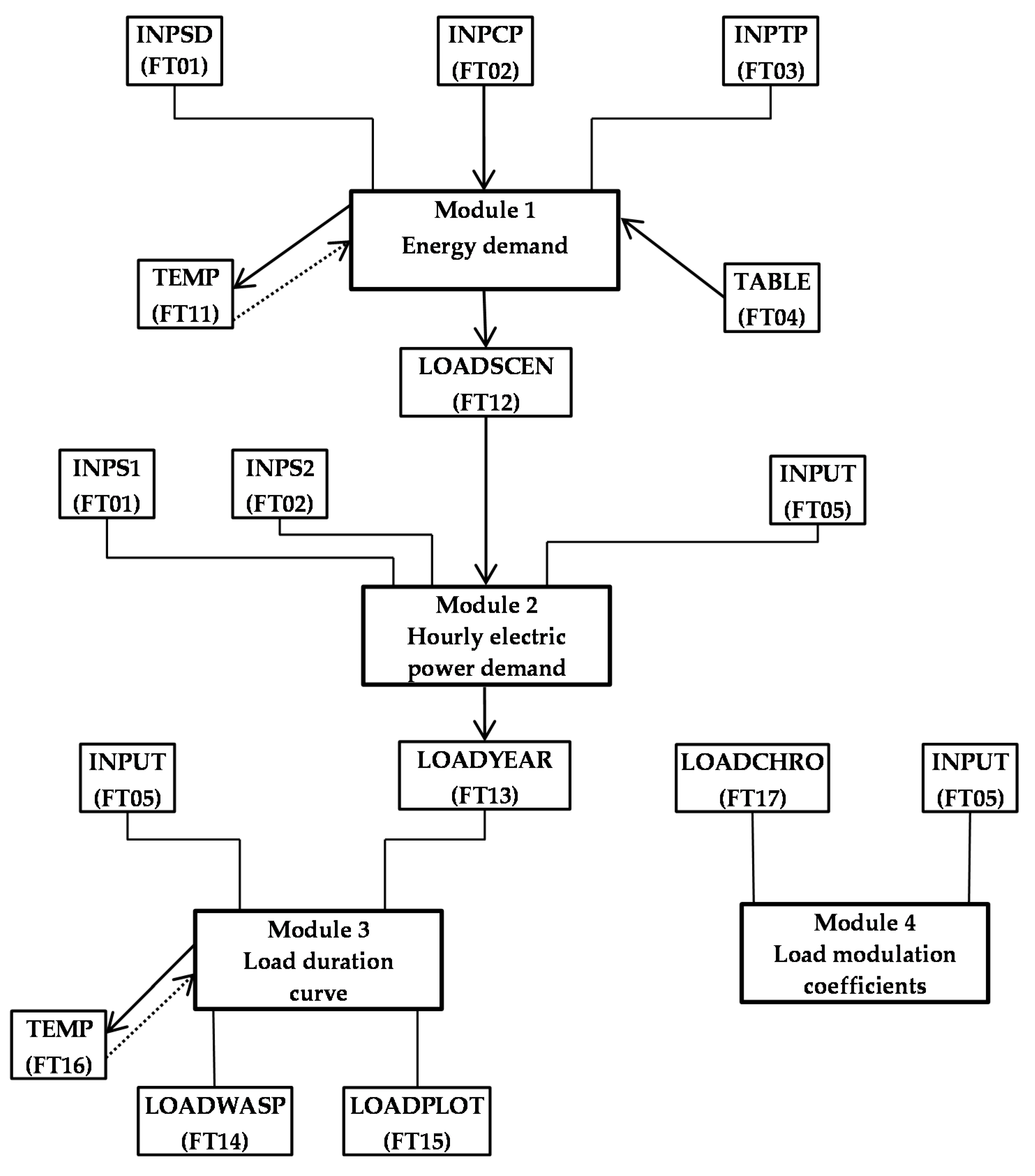
The general structure of MAED is shown in Figure 2, which also illustrates the flow of information from the various modules and associated data files [28].
The number assigned to each module indicates the proper sequence of their execution [28]:
Module 1 (Energy Demand Calculations) processes information describing the social, economic and technological scenario of development and calculates the total energy demand for the desired years. The breakdown of this demand by energy form and by economic sector considered is also provided as part of the results of the analysis. This module creates a file (FT12: “LOADSCEN”) to be used later by Module 2. A scratch file (FTll: “TEMP”) is also used as a temporary working file by Module 1.
Module 2 (Hourly Electric Power Demand) uses the total annual demand of electricity for each sector (contained in file “LOADSCEN”) to determine the total electric power demand for each hour of the year or, in other words, the hourly electric load which is imposed on the power system under consideration. During its execution, this module creates a file (FT13: “LOADYEAR”) to be used by Module 3.
Module 3 (Electric Load Duration Curve) uses the hourly loads (contained in file “LOADYEAR”) to produce the load duration curve of the power system as required for the execution of a WASP study. Two output files are created by this module during execution. The first one, file (FT14: “LOADWASP”), contains the WASP input data, and the second (FT15: “LOADPLOT”) contains the same information but is presented in a different format as required for plotting the load duration curve. (At IAEA, plotting of curves is done by means of a software product, i.e., TELL-A-GRAF, marketed by Integrated Software Systems Corporation, U.S.A.)
Module 4 (Load Modulation Coefficients) is an auxiliary module of MAED-1 which may be used to analyze the past evolution of the coefficients, describing the variation of the hourly electric loads based on load curves determined from statistical data. An additional input file, i.e., “LOADCHRO”, with the chronological electric power demand hour-by-hour for past years of statistics is required for executing this module.

4. Scenarios and Background Information for MAED

It is necessary to analyze the evolution of energy demand by building scenarios for future development. Scenarios are not predictions or forecasts but are descriptions of images of the future, created from models that reflect different perspectives on the past, present and future.
For the case of Mali, three scenarios were adopted, including one reference scenario and two alternative scenarios (Low and High):
Reference scenario: Reflects the historical trend (from 2014 to 2019) taking into account the variations in GDP.
Low scenario: Under this scenario, climate change, socio-political and economic crises, and threats to territorial integrity will continue to plague Mali.
High scenario: Reflects a more optimistic view of the future, according to state forecasts.
The three scenarios were developed based on four groups of coherent hypotheses concerning:
Demographic evolution;
Economic development;
Lifestyle change;
Technological change.

4.1. Input Data from the National Energy Authority of Mali for MAED_D

4.1.1. Assumptions on Demographic Development

The demographic change assumption is identical for all scenarios. The population of the Taoussa area was 0.754 million people in 2020, and more than 50% of them live in rural areas. The socio-demographic characteristics of the population are summarized in Table 2 below.

4.1.2. Assumptions on Economic Development Assumptions

These three scenarios share certain government economic policy objectives, namely: poverty eradication, infrastructure development, food security, economic stabilization (inflation, internal and external debt), etc.
The GDP growth rates of the three scenarios are:
Reference scenario: 3.6% until the year 2025, 4.4% during 2026–2030 and 4.6% during 2031–2035 (historical trend);
Low scenario: 2% until the year 2025, 2.5% during 2026–2030 and 2.5% during 2031–2035 (crisis situation);
High scenario: 6.1% until the year 2025, 6.5% during 2026–2030 and 6.4% during 2031–2035 (government objectives).
Table 3 summarized the general information on the economic sectors for the reference scenario.

4.1.3. Assumptions on Lifestyle Change

A common assumption for all scenarios regarding the number of persons per household:
Urban areas: 5.9 until 2025, 5.7 from 2026 to 2030 and 5.0 after 2030;
Rural areas: 10 until 2025, 9 from 2026 to 2030 and 8 after 2030.
The Taoussa area electricity penetration by scenario is shown in Table 4. In 2020, it was about 41%, with 62% in urban areas and 20% in rural areas.
The electricity consumption per dwelling for electrical appliances and lighting by scenario is given in Table 5.

4.1.4. Assumptions on Technological Development

Growth in the energy intensities of fuels and specific uses of electricity in all sectors is based on the following aspects:
Introduction of agricultural machinery in Agriculture;
Mechanization of construction and mining activities;
Introduction of engines and other supplementary equipment in the manufacturing industry;
Introduction of IT equipment and other technologies in services.
Thermal process efficiencies will increase in all scenarios, but at different rates:
Low Scenario: more pessimistic than the historical pace;
Reference scenario: keep the historical pace;
High Scenario: more optimistic than the historical pace.
Traditional fuels will be replaced by commercial fossil fuels, but at different rates:
Low scenario: at a slow pace;
Reference scenario: at a moderate pace;
High Scenario: at an accelerated pace.

4.1.5. Technological Parameters

The energy demand is calculated separately for four major aggregated sectors: industry, transportation, service and household. The calculation of the energy demand of each sector is performed in a similar procedure, in which the demand for each end-use category of energy is driven by one or several socioeconomic and technological parameters whose values are given as part of the scenarios.
The technological parameters are:
Industry (ACM (agriculture, construction, mining) and manufacturing)
Energy intensities ACM and manufacturing, efficiencies and penetrations in ACM and efficiencies, penetrations and factors in manufacturing.
Transport
Generation of freight kilometers, modal split of freight transportation, energy intensities, modal split of cars intercity transportation, load factors (person per mode type), and energy consumption of international transportation.
Household
Shares by dwelling type, dwelling sizes by dwelling type, dwelling factors for water heating, dwelling factors for cooking, dwelling factors for air conditioning, dwelling factors for appliances, dwelling factors for lighting and energy intensities.
Service sector
Labor force, floor area per employee, factor for air conditioning, energy intensities, penetration and efficiencies.

4.2. Input Data for MAED_EL

Related input parameters are shown in Table 6, Table 7 and Table 8.

4.3. Coefficients Definition of the Base Year (2019)

We used relevant historical consumption from annual activity report in reference [29] to elaborate the Figure 3 and Figure 4 and Table 9. The Figure 3 shows the hourly load curve of the Taoussa area for the base year 2019. It allows for a more detailed analysis (hour by hour) of consumption. It can be seen that the minimum load, the electricity consumption, is 0.91 MW. After all, the peak load should only be 5.90 MW.
Figure 4 and Table 9 show the weekly, daily and hourly load coefficients calculated over the hourly load curve during the base year.

5. Results and Discussions

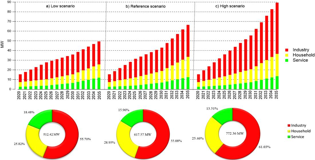
The main objective of the project was to contribute to the sustainable development of the regions of northern Mali, as well as poverty reduction, environmental management and specifically for the long term, to produce 332.57 GWh/year, 472.61 GWh/year and 647.02 GWh/year electricity in the low, reference and high scenarios by 2035.

5.1. Final Electricity Demand by Sector

In Table 10, Table 11 and Table 12, electricity demand in 2020 was 15.41 MW (106.84 GWh) for all scenarios; the average annual growth rate of electricity demand is slightly higher during the 2021–2035 period, 8.13% in average from 17.88 MW (117.28 GWh) to 49.40 MW (332.57 GWh) for low LS, 10.31% in average from 18.62 MW (129.97 GWh) to 66.46 MW (472.61 GWh) for RS and 12.56% in average from 19.53 MW (136.65 GWh) to 89.47.01 MW (647.02 GWh) for HS. The share by sector is 56.77% in industry, 25.60% in household and 17.63% in service for LS, 56.13% in industry, 28.55% in household and 15.31% in service for RS and 61.16% in industry, 25.67% in household and 13.17% in service for RS, respectively. We construe that electricity demand for the industry sector will be equal to household and service demand.

5.2. Demography and Comparative Evolution of GDP by Scenario

The projection for the total population and GDP of the Taoussa area are presented in Table 11. It has been found that the demography will grow annually at an average rate of 3.97% from 0.754 million people in 2020 to 1.351 million people in 2035. GDP in 2020 was USD 1.30 billio for all scenarios and the annual average GDP growth rates will be 2.33% from USD 1.33 billion in 2021 to USD 1.84 billion in 2035, 4.20% from USD 1.35 billion in 2021 to USD 2.41 billion in 2035 and 6.33% from USD 1.39 billion in 2021 to USD 3.27 billion in 2035 for LS, RS and HS, respectively.
The forecast annual average growth rate of GDP/Cap and electricity demand/Cap is shown in Table 11. During 2020–2035, the GDP/Cap will be 4% from 0.08 kWh/USD to 0.19 kWh/USD for the LS, 6.3% from 0.08 kWh/USD to 0.20 kWh/USD for the RS and 8.5% from 0.08 kWh/USD to 0.19 kWh/USD for the HS, whereas the electricity demand/Cap is projected to account for 5.6% from 0.14 MWh/cap to 0.25 MWh/cap, 6.1% from 0.14 MWh/cap to 0.35 MWh/cap and 6% from 0.14 MWh/cap to 0.47 MWh/cap in the LS, RS and HS, respectively.

5.3. Total Annual Electric Energy Demand and Peak Load

Simulation of total hourly electricity demand forecast for the period from 2020–2035 must meet the peak load time, a short period of critical time during which electricity consumption is highest within a year and could have a strong influence on the reliability of electricity supply.
In Table 12, the times ahead of system peak load illustrate that the average annual growth rate of the system peak between 2020 and 2035 represents 7.92% in the Low scenario; in this case, the system peak demand will increase from 20.8 MW in 2020 to 64.88 MW in 2035. The system peak electricity demand time of day in the Reference scenario is forecasted to increase to 10.53% per year from beginning to end of the study period and from 25.35 MW in 2021 to 92.2 MW in 2035. On the other hand, the system peak demand in the High scenario is forecasted to increase at approximately 12.91% annually, from 26.65 MW in 2021 to 126.22 MW in 2035.
The information on total electric energy by month in Gwh for all the scenarios is presented in (Appendix A). This allows for visualizing the proportion of months in which consumption is higher than a certain level of power; the lowest consumption is in the cool season in January from 4.89 GWh in 2020 for all scenarios to 15.18 GWh for LS, 21.57 GWh for RS and 29.53 GWh for HS in 2035, respectively, while the month of high consumption is in the hot season in May from 12.40 GWh in 2020 for all scenario to 38.37 GWh for LS, 54.52 GWh for RS and 74.64 GWh in 2035, respectively.

5.4. Comparative Evolution between Annual Electricity Demand and Peak Load by Scenario

The difference between the annual electricity demand and peak load forecasts was relatively big for all scenarios. This difference will increase at an average annual growth rate of about 7.49%, 10.31% and 13.87% in the Low scenario from 5.39 MW in 2020 to 15.48 MW by 2035, in the Reference scenario from 6.73 MW in 2021 to 25.74 MW by 2035, and in the High scenario from 7.12 MW in 2020 to 36.75 MW by 2035, respectively.
The ways to reduce the electricity demand during peak load include replacing energy-intensive appliances with more energy-efficient ones, shifting the operation of electricity-consuming equipment during a peak period to periods of inactivity (off-peak hours), organizing the implementation of equipment according to a plan, raising awareness of the population towards energy saving and relieving certain groups of necessary equipment.

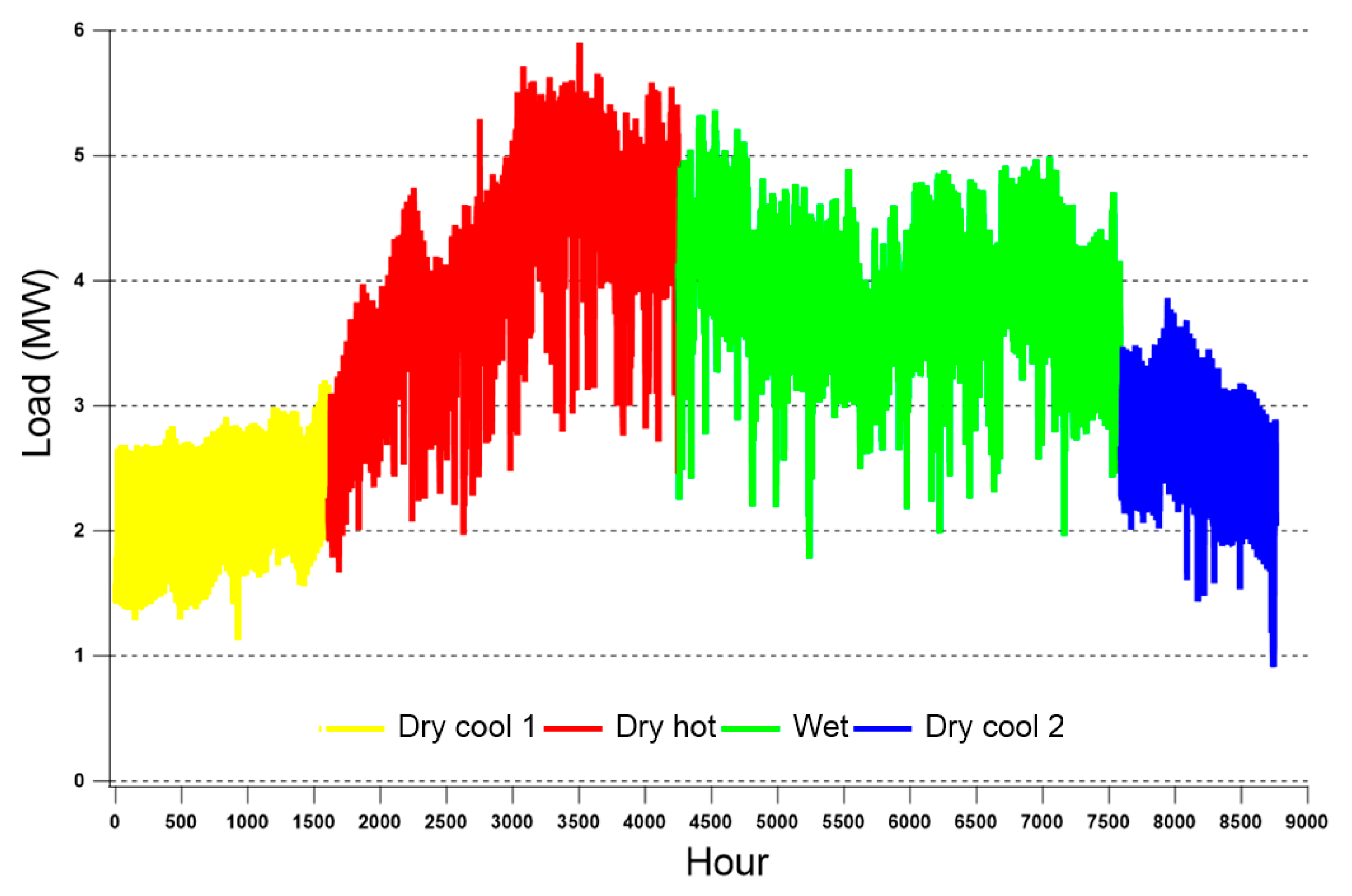
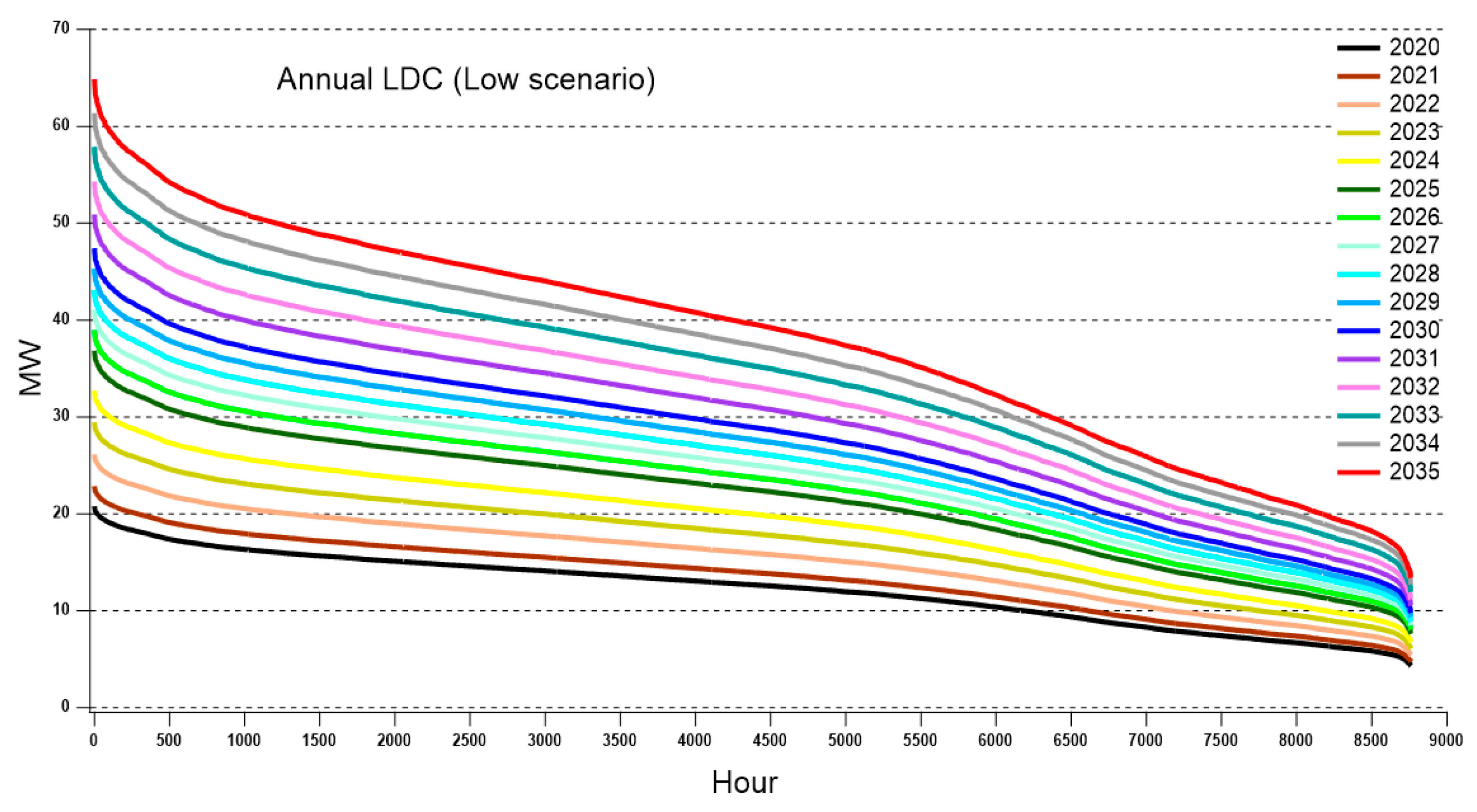
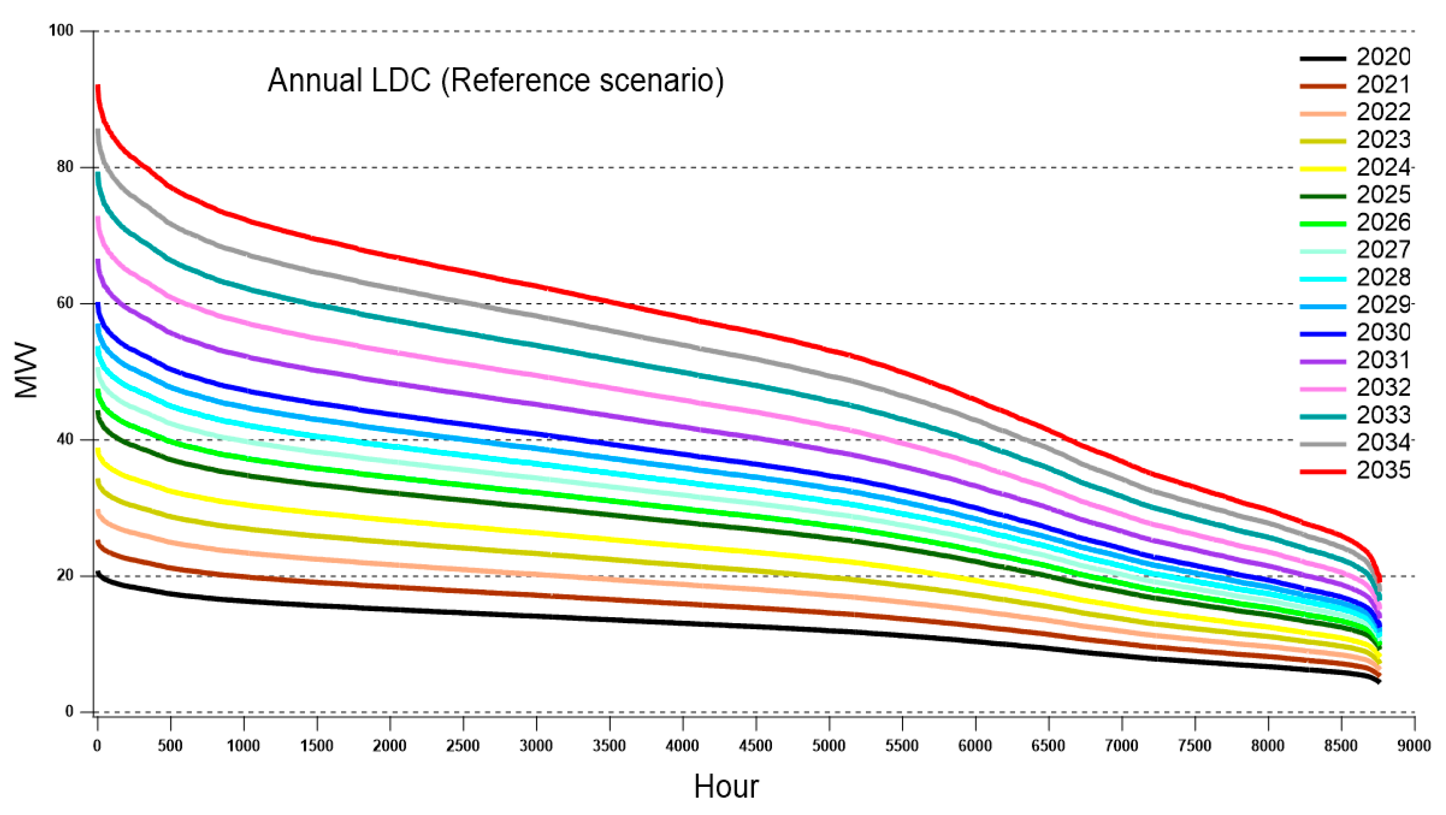
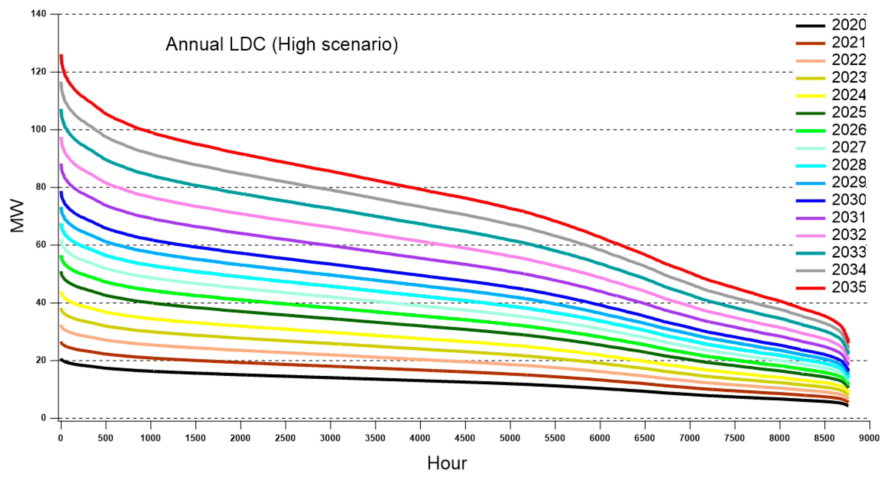
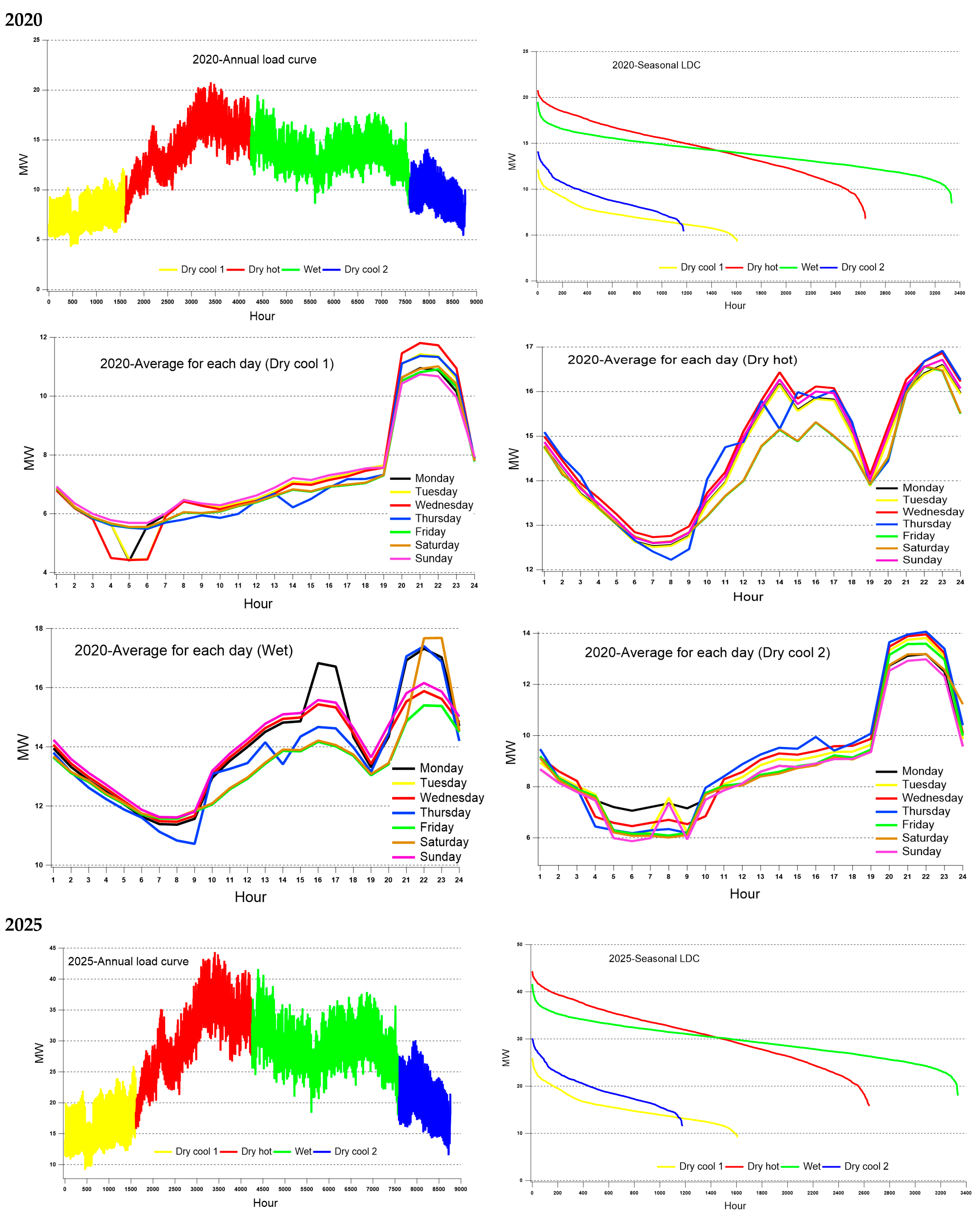
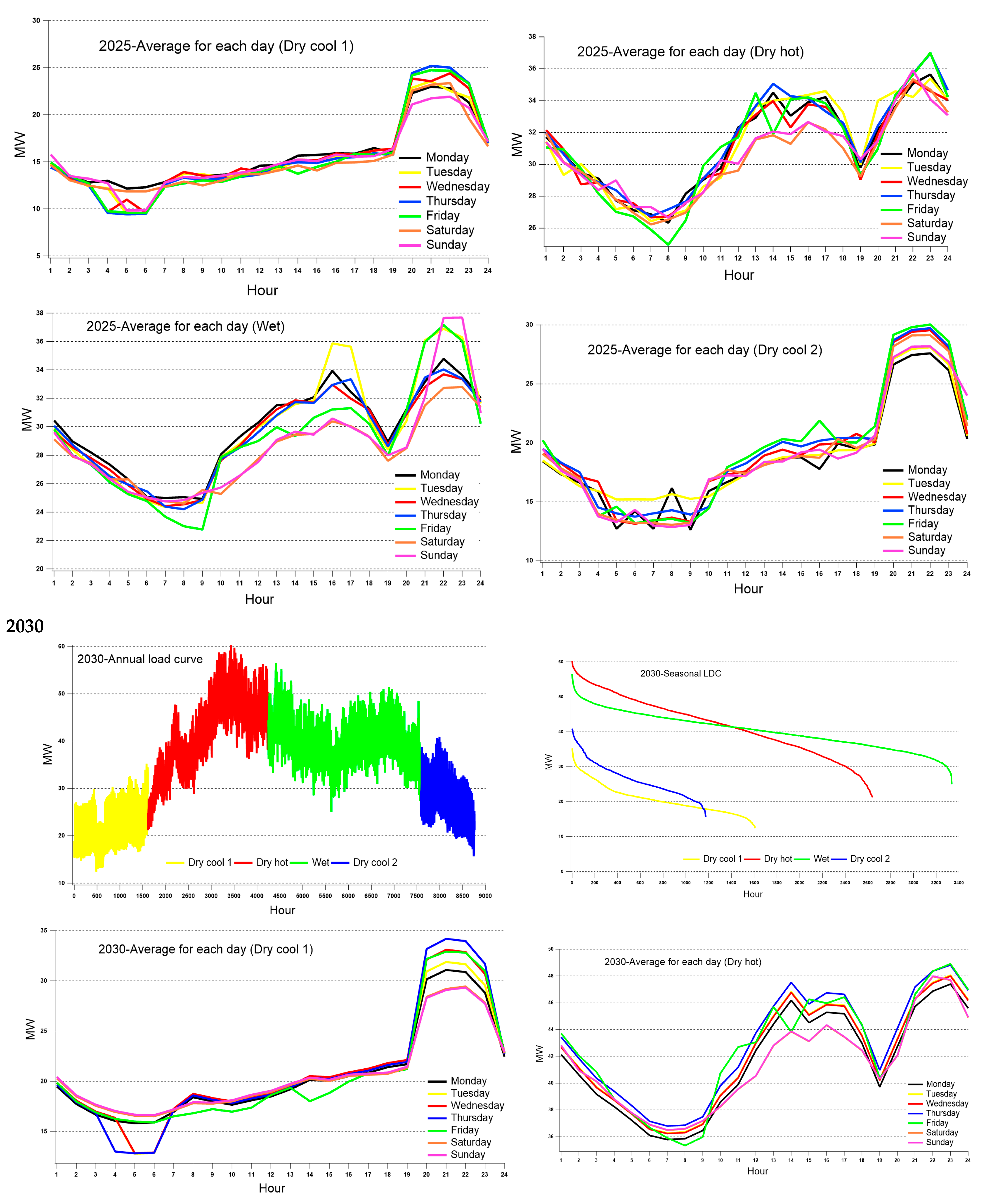
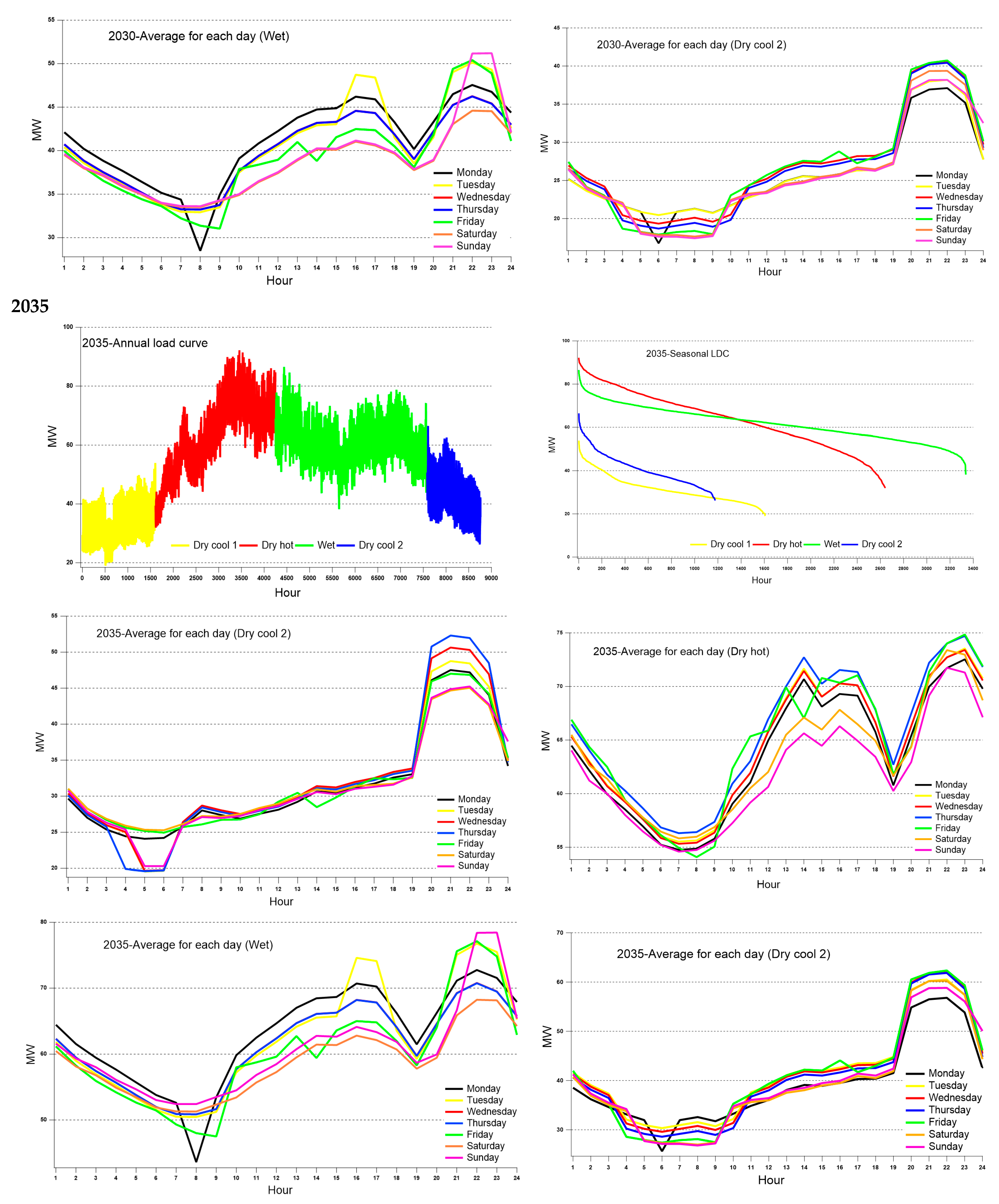
5.5. Annual Load Duration Curves by Scenario

From Figure 5, Figure 6 and Figure 7 show the annual load duration curves (LDC) permit to view the proportion of the time during which the consumption is peak load or minimum load. It is shown that the peak loads during 2020 to 2035 are in the hot dry season between 17–23 May at 9:00 p.m., and the minimum load is between 15–21 January at 7:00 a.m.
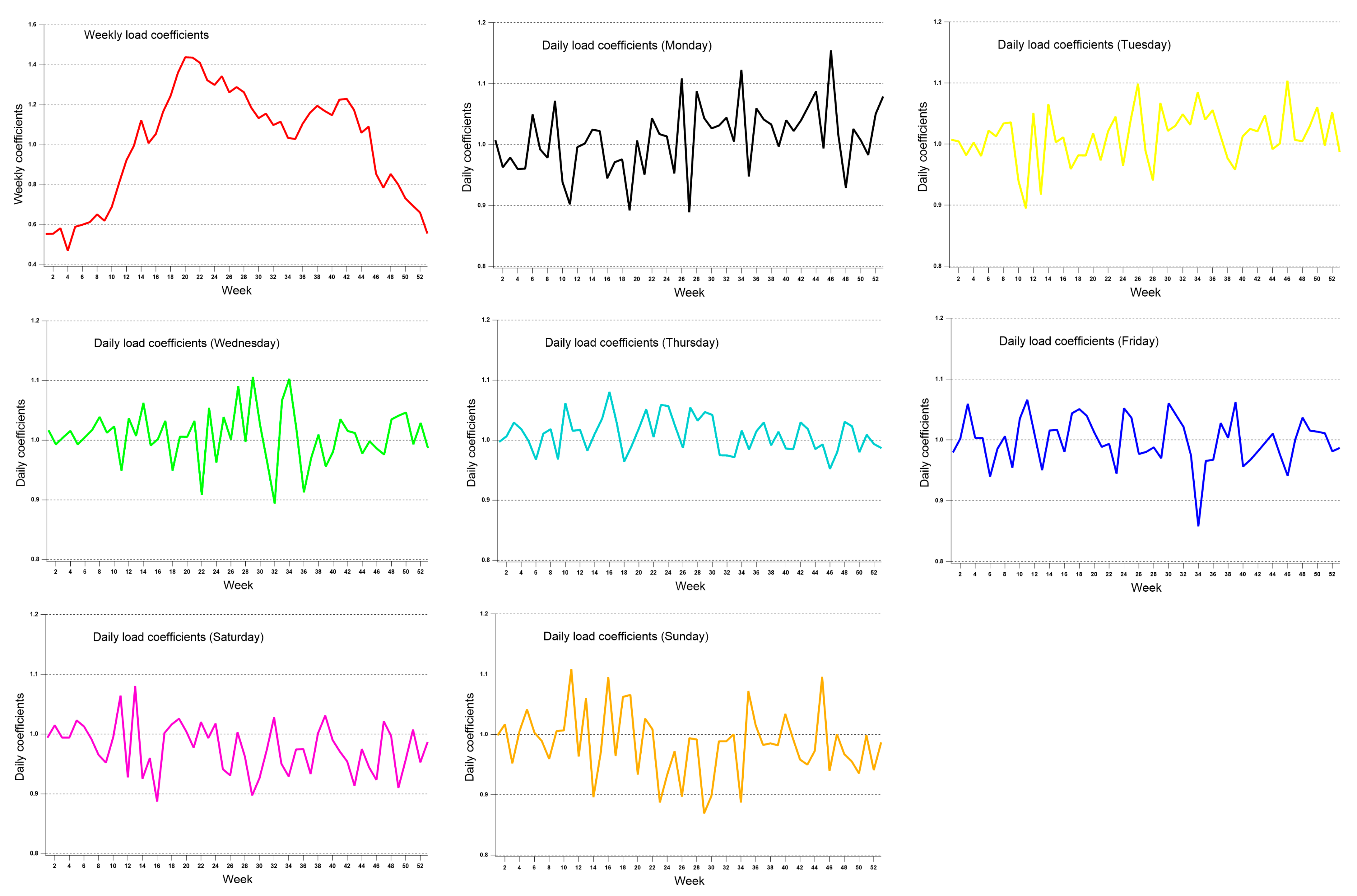
The electricity demand system load is divided usually into four seasons; Figure A1 shows the average electricity demand for each day by season at the same time. In the Taoussa area, there are three types of days (workdays, Fridays and weekends); the workdays include four days (Monday to Thursday) and the weekend includes two days (Saturday and Sunday). Taoussa’s electricity demand is virtually the same for all-day types in the dry cool 1 season and dry cool 2 season. Generally, for all-day types, peak hours are from 8:00 p.m. to 11:00 p.m., and off-peak hours are from 3:00 a.m. to 9:00 a.m.
Future work will be based on the hybrid renewable energies (solar power, hydroelectric power, wind power) optimization technique using the MESSAGE model to satisfy this electricity demand.

6. Conclusions

During the study period 2020–2035, MAED analysis has shown that the GDP, electric capacity and electricity demand will increase to USD 1.84 billion and 49.40 MW (332.57 GWh) for the Low scenario (LS), USD 2.41 billion and 66.46 MW (472.61 GWh) for the Reference scenario (RS), and USD 3.27 billion, 89.47 MW (635 GWh) for the High scenario (HS), respectively. The total electricity demand in the Taoussa area increased at an average rate of 8.13% in the LS, 10.31% in the RS and 12.56% in the HS in all sectors. The demographic was identical for all scenarios and will increase to 1.351 million people.
The industry sector (including manufacturing, construction, mining and agriculture) will be the biggest electricity consumer of the Taoussa area. Under the calculated growth, the system peak load in the planning horizon and the electricity peak demand is expected to grow at about 7.92%, 10.53% and 12.91% corresponding respectively to the three scenarios (LS, RS and HS). The days of peak load are in the hot dry season between 17–23 in May. The growth rate has gradually increased year by year. Based on the calculation results, the following conclusions can be drawn. There is a need for energy conservation and energy efficiency measures in all electricity sectors, which can reduce the future electricity demand, decrease the greenhouse gas emissions and consequently fight against climate change and bring down the public investment in the electricity production in the Taoussa area.

Author Contributions

Conceptualization, M.K.; supervision, Y.L. and S.D.; All authors have read and agreed to the published version of the manuscript.

Funding

This research received no external funding.

Institutional Review Board Statement

Not applicable.

Informed Consent Statement

Not applicable.

Data Availability Statement

Not applicable.

Acknowledgments

The first author extends his thanks to Mario Tot from the IAEA for his help and support in the application of the energy demand assessment tool MAED. Thanks also go to Adama Mody DIAKITE, chief, division of studies and planning, national energy authority of Mali and Isaac Goita from Taoussa planning authority for their cooperation during the data collection.

Conflicts of Interest

The authors declare no conflict of interest.

Appendix A. Summary Annual Electricity Demand

Table A1. Peak load, electric energy and load factor.
YearSeasonMaximum Load
(MW)
Relation to Annual PeakEnergy (GWh)Load Factor (%)
ScenarioScenarioScenarioScenario
LowReferenceHighLowReferenceHighLowReferenceHighLowReferenceHigh
2020Dry cool 112.1712.1712.170.580.580.5811.7311.7311.7359.0659.0659.06
Dry hot20.820.820.811138.3538.3538.3569.8369.8369.83
Wet19.5219.5219.520.940.940.9446.1546.1546.1570.8770.8770.87
Dry cool 214.1214.1214.120.680.680.6810.610.610.663.8463.8463.84
2021Dry cool 113.3814.8215.590.580.580.5812.7714.1514.8859.3759.3759.37
Dry hot22.8725.3526.6511142.3146.8949.370.0770.0770.07
Wet21.4623.7825.010.940.940.9450.6356.158.9970.7170.7170.71
Dry cool 215.5317.2118.090.680.680.6811.5812.8313.4963.4163.4163.41
2022Dry cool 115.317.4618.980.580.580.5814.6716.7418.2159.6459.6459.64
Dry hot26.1629.8632.4611148.5455.3960.2370.2870.2870.28
Wet24.5528.0230.460.940.940.9457.7965.9471.770.5570.5570.55
Dry cool 217.7620.2722.040.680.680.6813.1715.0316.3463.0563.0563.05
2023Dry cool 118.0721.0923.490.610.610.6116.6119.3821.5857.1557.1557.15
Dry hot29.4534.3638.2711154.8163.9471.2170.4870.4870.48
Wet27.6432.2535.910.940.940.9464.9175.7384.3570.470.470.4
Dry cool 219.9923.3325.980.680.680.6814.7417.1919.1562.6762.6762.67
2024Dry cool 119.1322.7125.760.580.580.5818.3221.7524.6758.6858.6858.68
Dry hot32.7238.8444.0511159.817180.5269.2569.2569.25
Wet30.736.4441.330.940.940.9472.9686.6198.2271.2471.2471.24
Dry cool 222.2126.3629.90.680.680.6816.8620.0122.764.5664.5664.56
2025Dry cool 121.5625.9529.810.580.580.5820.4224.5828.2458.9158.9158.91
Dry hot36.8644.3750.9811167.6881.4793.5969.5569.5569.55
Wet34.5941.6447.830.940.940.948298.7113.3971.0671.0671.06
Dry cool 225.0230.1234.60.680.680.6818.8922.7426.1264.1964.1964.19
2026Dry cool 122.7927.833.060.580.580.5821.6626.4231.4259.1159.1159.11
Dry hot38.9747.5456.5311171.8487.64104.2269.8369.8369.83
Wet36.5744.6153.050.940.940.9486.46105.47125.4270.8770.8770.87
Dry cool 226.4532.2738.380.680.680.6819.8624.2228.8163.8463.8463.84
2027Dry cool 124.0229.6636.310.580.580.5822.9328.3134.6759.3759.3759.37
Dry hot41.0850.7162.0911175.9893.8114.8670.0770.0770.07
Wet38.5547.5858.270.940.940.9490.92112.24137.4470.7170.7170.71
Dry cool 227.8834.4242.150.680.680.6820.7925.6731.4363.4163.4163.41
2028Dry cool 126.4633.0141.440.610.610.6124.6430.7538.6157.0857.0857.08
Dry hot43.1153.7967.5411180.22100.08125.6770.4870.4870.48
Wet40.4650.4763.380.940.940.9495.02118.54148.8570.470.470.4
Dry cool 229.2736.5145.850.680.680.6821.5726.9133.7962.6762.6762.67
2029Dry cool 126.533.3842.830.580.580.5824.9331.440.2958.558.558.5
Dry hot45.3157.0773.2411182.49103.9133.3468.9668.9668.96
Wet42.5253.5568.730.940.940.94101.25127.53163.6671.3871.3871.38
Dry cool 232.6541.1352.780.720.720.7223.629.7338.1561.4661.4661.46
2030Dry cool 127.7335.2346.090.580.580.5826.1933.2743.5258.7258.7258.72
Dry hot47.4260.2578.8111186.7110.15144.0869.2569.2569.25
Wet44.556.5373.950.940.940.94105.76134.36175.7571.2471.2471.24
Dry cool 232.1940.953.50.680.680.6824.4431.0540.6264.5664.5664.56
2031Dry cool 129.7738.9651.630.580.580.5828.236.9148.958.9158.9158.91
Dry hot50.9166.6388.2811193.46122.32162.0869.5569.5569.55
Wet47.7762.5282.830.940.940.94113.23148.2196.3671.0671.0671.06
Dry cool 234.5645.2359.920.680.680.6826.0934.1445.2364.1964.1964.19
2032Dry cool 131.7642.6357.080.580.580.5830.7441.2655.2459.3159.3159.31
Dry hot54.3172.8997.6111100.45134.83180.5370.0770.0770.07
Wet50.9668.491.580.940.940.94120.2161.34216.0270.7170.7170.71
Dry cool 236.8649.4866.250.680.680.6827.4936.949.463.4163.4163.41
2033Dry cool 133.8446.4262.70.580.580.5832.4644.5260.1359.6459.6459.64
Dry hot57.8779.38107.21111107.37147.29198.9270.2870.2870.28
Wet54.374.49100.60.940.940.94127.81175.32236.7870.5570.5570.55
Dry cool 239.2853.8972.780.680.680.6829.1339.9653.9663.0563.0563.05
2034Dry cool 137.6552.6371.60.610.610.6134.648.3665.857.1557.1557.15
Dry hot61.3585.76116.68111114.16159.57217.170.4870.4870.48
Wet57.5780.48109.480.940.940.94135.22189257.1470.470.470.4
Dry cool 241.6558.2279.20.680.680.6830.742.9158.3862.6762.6762.67
2035Dry cool 137.9453.9273.820.580.580.5835.6950.7269.4458.558.558.5
Dry hot64.8892.2126.22111118.11167.85229.7968.9668.9668.96
Wet60.8886.51118.440.940.940.94144.97206.02282.0471.3871.3871.38
Dry cool 246.7666.4490.960.720.720.7233.7948.0265.7461.4661.4661.46
Table A2. Total electric energy by month (Gwh): Low scenario.
YearMonth
Jan.Feb.Mar.Apr.MayJuneJulyAug.Sep.Oct.Nov.Dec.
20204.895.047.029.5212.4011.1910.859.699.9910.568.187.50
20215.355.477.5810.3513.5312.0711.8510.6610.9111.599.298.63
20226.126.268.6311.8415.4813.6413.5212.1912.4813.2610.799.95
20236.897.059.6513.3417.4315.1615.2013.7314.0514.9312.2811.37
20247.687.9311.0314.9719.4917.5917.0615.2415.7116.6012.8711.79
20258.628.8112.2116.6821.8019.4519.0917.1717.5818.6814.9813.91
20269.129.3212.8517.6423.0520.3120.1418.1618.5919.7516.0714.82
20279.619.8213.4618.5924.3021.1421.1919.1419.5920.8217.1215.85
202810.1310.4614.5519.7425.7023.1922.5020.0920.7121.8816.9615.54
202910.6010.8315.0120.5026.7923.9023.4621.1121.6022.9618.4117.09
203011.0911.3415.6321.4628.0424.7124.5022.0922.6124.0319.5518.03
203111.9112.1716.6723.0430.1126.1926.2523.7224.2825.8021.2119.64
203212.7513.1718.3224.8632.3729.2028.3325.3026.0827.5621.3619.58
203313.5413.8419.1826.2034.2430.5429.9826.9727.6029.3423.5221.84
203414.3614.6720.2327.7836.3031.9831.7228.5929.2731.1125.3123.34
203515.1815.5121.2529.3638.3733.3733.4530.2230.9332.8827.0325.02
Table A3. Total electric energy by month (Gwh): Reference scenario.
YearMonth
Jan.Feb.Mar.Apr.MayJuneJul.Aug.Sep.Oct.Nov.Dec.
20204.895.047.029.5212.4011.1910.859.699.9910.568.187.50
20215.936.068.4011.4714.9913.3713.1311.8112.0912.8510.309.57
20226.997.149.8513.5217.6615.5615.4313.9114.2415.1412.3211.36
20238.048.2211.2615.5620.3317.6817.7316.0116.3917.4214.3313.26
20249.129.4113.1017.7723.1420.8820.2518.0918.6519.7015.2714.00
202510.3810.6114.7020.0826.2423.4122.9820.6721.1622.4918.0316.74
202611.1211.3715.6721.5228.1224.7824.5722.1522.6724.1019.6118.08
202711.8712.1316.6122.9530.0026.0926.1623.6324.1925.7021.1419.56
202812.6313.0518.1524.6332.0628.9328.0725.0625.8427.3021.1619.39
202913.3513.6418.9025.8233.7530.1029.5526.5827.2128.9223.1821.53
203014.0914.4019.8627.2635.6331.3931.1328.0628.7230.5324.8422.91
203115.5915.9321.8230.1539.4134.2734.3631.0431.7733.7727.7725.70
203217.1217.6724.5933.3743.4439.1938.0333.9635.0136.9928.6826.28
203318.5818.9826.3135.9446.9641.8941.1236.9937.8640.2432.2629.96
203420.0720.5128.2838.8350.7444.7144.3439.9740.9143.4835.3832.63
203521.5722.0430.1941.7254.5247.4247.5442.9543.9646.7238.4235.56
Table A4. Total electric energy by month (Gwh): High scenario.
YearMonth
Jan.Feb.Mar.Apr.MayJuneJul.Aug.Sep.Oct.Nov.Dec.
20204.895.047.029.5212.4011.1910.859.699.9910.568.187.50
20216.246.378.8312.0615.7614.0613.8012.4212.7113.5110.8310.06
20227.607.7610.7014.7019.2016.9216.7815.1315.4816.4613.3912.35
20238.969.1512.5417.3322.6419.7019.7417.8418.2619.4015.9614.77
202410.3410.6814.8520.1626.2423.6722.9720.5121.1522.3517.3215.87
202511.9312.1916.8923.0730.1526.8926.4023.7524.3125.8320.7119.23
202613.2313.5218.6425.5933.4429.4629.2226.3426.9628.6523.3221.50
202714.5314.8520.3428.1136.7331.9532.0328.9329.6231.4825.8823.96
202815.8616.3822.7930.9240.2636.3235.2431.4732.4534.2826.5824.35
202917.1317.5124.2633.1443.3138.6337.9234.1134.9237.1129.7527.63
203018.4318.8425.9835.6646.6041.0640.7236.7137.5739.9332.4929.97
203120.6521.1128.9239.9552.2145.4145.5241.1342.1044.7436.7934.05
203222.9223.6632.9344.6858.1752.4850.9245.4746.8849.5338.3935.18
203325.0925.6435.5348.5363.4256.5755.5449.9651.1454.3543.5740.46
203427.3127.9138.4852.8269.0360.8360.3254.3855.6659.1548.1444.39
203529.5330.1741.3457.1274.6464.9265.0858.7960.1863.9652.5948.68
Figure A1. Annual load curve, seasonal load duration curve and daily load curve (Reference scenario).
Energies 14 08515 g0a1aEnergies 14 08515 g0a1bEnergies 14 08515 g0a1c

References

  1. IAEA. Indicators for Sustainable Energy Development; IAEA: Vienna, Austria, 2002. [Google Scholar]
  2. Bhattacharyya, S.C. Energy Demand Models for Policy Formulation: A Comparative Study of Energy Demand Models; Centre for Energy, Petroleum and Mineral Law & Policy (CEPMLP), Dundee University: Dundee, UK, 2009; Available online: https://openknowledge.worldbank.org/bitstream/handle/10986/4061/WPS4866.pdf (accessed on 5 October 2021).
  3. IAEA. Facilitate and Supervise Fellowships on IAEA’s Model for Energy Demand Analysis (MAED) for Mali and Senegal; IAEA: Vienna, Austria, 2012. [Google Scholar]
  4. Soliman, S.A.-H.; Al-Kandari, A.M. Electrical Load Forecasting: Modeling and Model Construction; Elsevier: Amsterdam, The Netherlands, 2010. [Google Scholar]
  5. Song, Q.; Zhao, X.; Feng, Z.; An, Y.; Song, B. Hourly electric load forecasting algorithm based on echo state neural network. In Proceedings of the 2011 Chinese Control and Decision Conference (CCDC), Mianyang, China, 23–25 May 2011; pp. 3893–3897. [Google Scholar]
  6. Abdel-Aal, R. Univariate modeling and forecasting of monthly energy demand time series using abductive and neural networks. Comput. Ind. Eng. 2008, 54, 903–917. [Google Scholar] [CrossRef]
  7. Almazrouee, A.I.; Almeshal, A.M.; Almutairi, A.S.; Alenezi, M.R.; Alhajeri, S.N. Long-Term Forecasting of Electrical Loads in Kuwait Using Prophet and Holt–Winters Models. Appl. Sci. 2020, 10, 5627. [Google Scholar] [CrossRef]
  8. Yazici, I.; Temizer, L.; Beyca, O.F. Short Term Electricity Load Forecasting with a Nonlinear Autoregressive Neural Network with Exogenous Variables (NarxNet). In Lecture Notes in Management and Industrial Engineering; Springer: Singapore, 2019; pp. 259–270. [Google Scholar]
  9. Bunnoon, P.; Chalermyanont, K.; Limsakul, C. Mid-Term Load Forecasting: Level Suitably of Wavelet and Neural Network based on Factor Selection. Energy Procedia 2012, 14, 438–444. [Google Scholar] [CrossRef] [Green Version]
  10. Nia, A.R.; Awasthi, A.; Bhuiyan, N. Industry 4.0 and demand forecasting of the energy supply chain: A literature review. Comput. Ind. Eng. 2021, 154, 107128. [Google Scholar] [CrossRef]
  11. Ghalehkhondabi, I.; Ardjmand, E.; Weckman, G.R.; Young, W.A. An overview of energy demand forecasting methods published in 2005–2015. Energy Syst. 2017, 8, 411–447. [Google Scholar] [CrossRef]
  12. Jornaz, A.; Samaranayake, V.A. A Multi-Step Approach to Modeling the 24-hour Daily Profiles of Electricity Load using Daily Splines. Energies 2019, 12, 4169. [Google Scholar] [CrossRef] [Green Version]
  13. Kiprijanovska, I.; Stankoski, S.; Ilievski, I.; Jovanovski, S.; Gams, M.; Gjoreski, H. HousEEC: Day-Ahead Household Electrical Energy Consumption Forecasting Using Deep Learning. Energies 2020, 13, 2672. [Google Scholar] [CrossRef]
  14. Ali, D.; Yohanna, M.; Puwu, M.; Garkida, B. Pacific Science Review A: Natural Science and Engineering Long-term load forecast modelling using a fuzzy logic approach. Nat. Sci. Eng. 2016, 18, 123–127. [Google Scholar]
  15. Bano, H.; Tahir, A.; Ali, I.; Khan, R.J.U.H.; Haseeb, A.; Javaid, N. Electricity Load and Price Forecasting Using Enhanced Machine Learning Techniques. In International Conference on Innovative Mobile and Internet Services in Ubiquitous Computing; Springer: Singapore, 2019; pp. 255–267. [Google Scholar]
  16. Ouedraogo, N.S. Modeling sustainable long-term electricity supply-demand in Africa. Appl. Energy 2017, 190, 1047–1067. [Google Scholar] [CrossRef]
  17. Arora, S.; Taylor, J.W. Rule-based autoregressive moving average models for forecasting load on special days: A case study for France. Eur. J. Oper. Res. 2018, 266, 259–268. [Google Scholar] [CrossRef] [Green Version]
  18. Hainoun, A.; Seif-Eldin, M.; Almoustafa, S. Analysis of the Syrian long-term energy and electricity demand projection using the end-use methodology. Energy Policy 2006, 34, 1958–1970. [Google Scholar] [CrossRef]
  19. Yuksek, O.; Komurcu, M.I.; Yuksel, I.; Kaygusuz, K. Hydroelectric power: A key potential in meeting the long term electric energy demand of Turkey. Energy Policy 2006, 34, 3093–3103. [Google Scholar] [CrossRef]
  20. Kichonge, B.; John, G.; Mkilaha, I.; Hameer, S. Modelling of future energy demand for Tanzania. J. Energy Technol. Policy 2014, 4, 16–31. [Google Scholar]
  21. Hainoun, A. Construction of the hourly load curves and detecting the annual peak load of future Syrian electric power demand using bottom-up approach. Int. J. Electr. Power Energy Syst. 2009, 31, 1–12. [Google Scholar] [CrossRef]
  22. CSAO/OCDE. Malian Regions of Gao, Kidal and Timbuktu. National and Regional Perspectives. 2015. Available online: https://www.oecd.org/fr/csao/publications/Les-regions-maliennes-de-Gao-Kidal-et-Tombouctou.pdf (accessed on 5 October 2021).
  23. Global Water Initiative (GWI). Resettlement, Compensation and Population Rights in the Area of the Dam of Taoussa; GWI: Bamako, Mali, 2010; Available online: https://pubs.iied.org/sites/default/files/pdfs/migrate/G04213.pdf (accessed on 5 October 2021).
  24. Ministry of Mines. Natural Resources of Mali Officially Announced by the Government, Mali. 2011. Available online: http://www.communcommune.com/article-les-immenses-richesses-du-sous-sol-du-mali-114960898.html (accessed on 5 October 2021).
  25. Ministry of Mines, Energy and Water of Mali. National Energy Policy, Mali. 2006. Available online: https://www.compete-bioafrica.net/events/events2/mali/Session1-1-Diawara-COMPETE-WS-Mali-2008.pdf (accessed on 5 October 2021).
  26. IAEA. IAEA’s Energy Planning Tools; IAEA: Vienna, Austria, 2020. [Google Scholar]
  27. IAEA. User Manual, Model for Analysis of Energy Demand (MAED); IAEA: Vienna, Austria, 2006. [Google Scholar]
  28. IAEA. User Manual, Model for Analysis of Energy Demand (MAED_1); IAEA: Vienna, Austria, 1986. [Google Scholar]
  29. Electricity of Mali. Annual Activity Report. 2019. Available online: https://www.enerdata.net/estore/country-profiles/mali.html (accessed on 5 October 2021).
Figure 1. Location of Mali in West Africa [22].
Energies 14 08515 g001
Figure 2. Organization of the MAED computer program [28].
Energies 14 08515 g002
Figure 3. Hourly load curve (2019).
Energies 14 08515 g003
Figure 4. Weekly and daily load coefficient curves of consumption during the base year.
Energies 14 08515 g004
Figure 5. Annual load duration curve of the study period (Low scenario).
Energies 14 08515 g005
Figure 6. Annual load duration curve of the study period (Reference scenario).
Energies 14 08515 g006
Figure 7. Annual load duration curve of the study period (High scenario).
Energies 14 08515 g007
Table 1. Status of Taoussa’s energy potential.
Energy PotentialsQuantity
Biomass7 million tones
SolarElectric potential varies from 6 to 8 kWh/m2 per day
Hydro3.1 billion m3 of water, hydroelectric power 25 MW, annual power generation capacity 118 GWh and irrigation 139,000 ha
WindAverage wind speeds vary from 5 m/s to 7 m/s depending on the locality.
Uranium200 tones
Gas and petroleumAround 850,000 km2 of gas and oil potential
Source [23,24].
Table 2. Evolution of the demography in the Taoussa area.
ItemUnit2020202520302035
PopulationThousand754.073895.6021089.6371351.401
Population growth rate% per annum-3.5004.0004.400
Urban population ratio%42.00044.00046.00048.000
Number of people per household (urban)/6.0005.9005.7005.000
Number of urban householdsThousand52.78566.79182.616121.886
Rural population ratio%58.00056.00054.00052.000
Number of people per household (rural)/10.83010.0009.0008.000
Number of rural householdsThousand40.38449.25861.42382.527
Potential labor force ratio%51.00051.00054.00057.000
Participating labor force%49.30049.50052.50055.500
Active labor forceThousand189.597226.095290.223401.651
Population ratio in cities with public transport%25.00028.00028.66728.667
Population inside large citiesThousand188.518250.769293.468363.968
Table 3. Total GDP and GDP structure by main economic sectors for reference scenario.
ItemUnit2020202520302035
GDPUSD Billion1.301.551.922.41
GDP Growth rate% p.a.-3.64.44.6
GDP per capitaUSD Billion/Cap1.721.731.771.78
Sectorial shares of GDP
Agriculture%30.930.028.027.0
Construction%5.15.66.07.0
Mining%9.59.07.06.0
Manufacturing%21.521.522.023.0
Service%30.730.534.033.0
Energy%2.33.43.04.0
Total%100100100100
Table 4. Dwelling factor for appliances and lighting: electricity penetration.
AreaScenario2020202520302035
UrbanLow62%65%68%70%
Reference62%82%90%95%
High62%85%95%100%
RuralLow20%25%35%50%
Reference20%35%50%60%
High20%40%55%65%
Table 5. Dwelling factor for appliances and lighting: specific electricity requirements (kWh/dw/year).
AreaScenario2020202520302035
UrbanLow2131.232195.172261.022328.85
Reference2131.232237.792349.682467.17
High2131.232344.352578.792836.67
RuralLow763.24801.40841.47883.55
Reference763.24839.56923.521015.87
High763.24877.731009.381160.79
Table 6. Electricity supplied from the grid for each sector.
SectorsUnit2020202520302035
Industry%80808080
Household%50535353
Service%60656565
Table 7. Electricity transmission and distribution system losses.
IndustryHouseholdService
5%20%15%
Table 8. Calendar definitions.
SeasonStarting DateType of Days
Dry cool 11 JanuaryWorking days
Dry hot11 MarchFriday
Wet1 JulySaturday/Sunday/Holiday
Dry cool 218 November
Table 9. Hourly load coefficients for typical days by season.
HourSeason
Dry Cool 1Dry HotWetDry Cool 2
Working DayFridayWeekendWorking DayFridayWeekendWorking DayFridayWeekendWorking DayFridayWeekend
00.9681.0040.9981.0121.0291.0331.0171.0331.0301.0011.0301.042
10.8810.9090.9030.9760.9900.9870.9710.9870.9920.9400.9070.944
20.8280.8550.8540.9410.9620.9680.9380.9480.9700.8990.8640.897
30.7980.8210.8230.9190.9130.9350.9100.9190.9380.8600.8250.864
40.7860.8090.8060.8940.8880.9110.8790.8920.9140.8300.8070.834
50.7900.8030.8060.8670.8630.8900.8490.8720.8870.8140.7910.817
60.8420.8340.8390.8600.8460.8800.8300.8340.8760.8300.8060.816
70.9150.8500.8790.8610.8330.8830.8290.8110.8760.8460.8120.807
80.8940.8700.8750.8760.8500.8970.8430.8030.8940.8240.7930.820
90.8770.8580.8840.9270.9570.9230.9440.9840.9110.8630.8660.879
100.8990.8780.9110.9581.0060.9540.9860.9950.9500.9060.9140.911
110.9180.9420.9301.0191.0140.9781.0211.0080.9780.9370.9650.921
120.9540.9780.9611.0671.0771.0331.0581.0611.0160.9891.0070.960
131.0010.9100.9921.1101.0331.0581.0811.0021.0501.0161.0350.973
140.9950.9520.9821.0691.0901.0401.0841.0761.0471.0111.0310.998
151.0191.0091.0071.0881.0811.0691.1161.0991.0721.0261.0811.010
161.0361.0511.0161.0851.0931.0471.1091.0971.0591.0471.0231.046
171.0641.0521.0251.0321.0441.0231.0451.0461.0341.0481.0551.036
181.0791.0731.0630.9540.9490.9720.9700.9810.9811.0781.0961.072
191.3321.3461.3141.0270.9851.0151.0461.0741.0021.2671.2801.288
201.3721.3771.3501.0981.0961.1151.1231.1351.1151.3061.3081.331
211.3631.3721.3611.1261.1371.1571.1481.1581.1561.3131.3181.332
221.2721.2951.2871.1391.1531.1501.1291.1231.1571.2441.2551.270
231.1161.1531.1321.0951.1091.0821.0721.0601.0931.1031.1321.134
Table 10. Final electricity demand, percentage increase and shares by sector.
YearSectorFinal Electricity Demand (MW)% IncreaseShares By Sector (%)
ScenarioScenarioScenario
LowReferenceHighLowReferenceHighLowReferenceHigh
2020Industry8.068.068.06---52.2752.2752.27
Transport0.000.000.00---0.000.000.00
Household4.824.824.82---31.2831.2831.28
Service2.542.542.54---16.4616.4616.46
Total15.4115.4115.41---100.00100.00100.00
2021Industry9.9510.2910.9823.4927.7636.2855.6355.2856.21
Transport0.000.000.000.000.000.000.000.000.00
Household5.165.535.707.1214.7818.3628.8729.7229.21
Service2.772.792.859.2610.1112.2815.5015.0014.58
Total17.8818.6219.5316.0320.7926.73100.00100.00100.00
2022Industry11.8412.5313.9019.0221.7326.6258.1857.4158.78
Transport0.000.000.000.000.000.000.000.000.00
Household5.516.246.596.6512.8715.5127.0628.6227.87
Service3.013.053.168.479.1810.9414.7713.9713.36
Total20.3521.8223.6513.8117.2121.09100.00100.00100.00
2023Industry13.7314.7616.8215.9817.8521.0260.1758.9960.58
Transport0.000.000.000.000.000.000.000.000.00
Household5.856.967.486.2311.4113.4325.6327.8026.92
Service3.243.313.477.818.419.8614.2013.2112.50
Total22.8225.0227.7712.1414.6917.42100.00100.00100.00
2024Industry15.6217.0019.7413.7815.1517.3761.7760.2261.92
Transport0.000.000.000.000.000.000.000.000.00
Household6.197.678.365.8710.2411.8424.4927.1726.22
Service3.483.563.787.257.768.9713.7412.6211.86
Total25.2928.2331.8910.8212.8114.83100.00100.00100.00
2025Industry17.5219.2322.6712.1113.1514.8063.0961.1962.95
Transport0.000.000.000.000.000.000.000.000.00
Household6.548.389.255.549.2910.5923.5426.6625.68
Service3.713.824.096.767.208.2313.3612.1511.37
Total27.7631.4336.019.7711.3512.92100.00100.00100.00
2026Industry18.1120.2125.123.375.0510.8461.6359.8962.95
Transport0.000.000.000.000.000.000.000.000.00
Household7.009.1010.077.078.568.9523.8226.9725.24
Service4.274.434.7115.1916.1015.1814.5513.1411.81
Total29.3833.7439.915.827.3310.85100.00100.00100.00
2027Industry18.7021.1827.583.264.819.7860.3258.7662.95
Transport0.000.000.000.000.000.000.000.000.00
Household7.469.8210.906.607.898.2224.0727.2324.88
Service4.845.055.3313.1913.8713.1815.6114.0012.17
Total30.9936.0443.825.506.839.79100.00100.00100.00
2028Industry19.2922.1530.043.164.598.9159.1457.7662.94
Transport0.000.000.000.000.000.000.000.000.00
Household7.9210.5311.736.197.317.5924.2927.4724.58
Service5.405.665.9611.6512.1811.6416.5614.7712.48
Total32.6138.3547.735.216.398.92100.00100.00100.00
2029Industry19.8823.1232.503.064.398.1858.0856.8862.94
Transport0.000.000.000.000.000.000.000.000.00
Household8.3811.2512.565.836.817.0624.5027.6824.32
Service5.966.286.5810.4410.8610.4317.4315.4412.74
Total34.2240.6551.634.956.018.19100.00100.00100.00
2030Industry20.4724.1034.962.974.207.5657.1056.0962.94
Transport0.000.000.000.000.000.000.000.000.00
Household8.8511.9713.385.516.386.5924.6827.8624.10
Service6.536.897.209.459.799.4418.2216.0412.96
Total35.8442.9655.544.725.677.57100.00100.00100.00
2031Industry21.1325.9038.573.257.4910.3354.8154.3561.88
Transport0.000.000.000.000.000.000.000.000.00
Household9.8113.7515.3110.8614.8714.3825.4428.8524.56
Service7.618.018.4516.6416.2117.3419.7516.8113.55
Total38.5547.6662.337.5710.9412.22100.00100.00100.00
2032Industry21.8027.7042.183.156.969.3652.8252.9161.03
Transport0.000.000.000.000.000.000.000.000.00
Household10.7715.5317.239.7912.9512.5826.0929.6624.94
Service8.709.139.7014.2713.9514.7821.0917.4314.03
Total41.2652.3669.117.039.8610.89100.00100.00100.00
2033Industry22.4629.5145.793.056.518.5651.0851.7160.34
Transport0.000.000.000.000.000.000.000.000.00
Household11.7317.3119.168.9211.4611.1726.6730.3325.25
Service9.7910.2410.9412.4812.2412.8822.2617.9514.42
Total43.9757.0675.906.578.989.82100.00100.00100.00
2034Industry23.1331.3149.402.966.117.8949.5350.7059.75
Transport0.000.000.000.000.000.000.000.000.00
Household12.6919.0921.098.1910.2810.0527.1830.9125.50
Service10.8711.3612.1911.1010.9111.4123.2918.3914.75
Total46.6961.7682.686.178.248.94100.00100.00100.00
2035Industry23.7933.1153.022.885.767.3148.1649.8359.26
Transport0.000.000.000.000.000.000.000.000.00
Household13.6520.8723.017.579.329.1327.6331.4025.72
Service11.9612.4813.449.999.8310.2424.2118.7715.02
Total49.4066.4689.475.817.618.21100.00100.00100.00
Table 11. Evolution of the demography, GDP, final electricity demand per capita and per GDP by scenario.
YearDemography GDP [109 USD]Final Energy by Capital [MWh/Cap]Final Energy by GDP [kWh/US$]
ThousandLSRSHSLSRSHSLSRSHS
2020754.071.301.301.300.140.140.140.080.080.08
2021782.381.331.351.390.150.170.170.090.100.10
2022810.681.351.401.480.170.190.200.100.110.11
2023838.991.381.451.570.180.210.230.110.120.12
2024867.301.411.501.660.190.230.260.120.130.13
2025895.601.441.551.750.210.250.290.130.150.15
2026934.411.471.631.880.210.260.310.140.150.15
2027973.221.511.702.010.220.270.320.140.150.16
20281012.021.551.782.140.220.270.340.140.160.16
20291050.831.591.852.270.220.280.350.150.160.16
20301089.641.621.922.390.220.280.360.150.160.17
20311141.991.672.022.570.230.300.390.160.170.17
20321194.341.712.122.740.240.310.410.170.180.18
20331246.701.752.222.920.240.330.430.170.180.18
20341299.051.792.313.090.250.340.450.180.190.19
20351351.401.842.413.270.250.350.470.190.200.19
Table 12. Annual electric energy demand, peak load and increase ratio.
Low ScenarioReference ScenarioHigh Scenario
YearEnergy (GWh)Increase Ratio (%)Peak (MW)Increase Ratio (%)Energy (GWh)Increase Ratio (%)Peak (MW)Increase Ratio (%)Energy (GWh)Increase Ratio (%)Peak (MW)Increase Ratio (%)
2020106.84-20.8-106.84-20.8-106.84-20.8-
2021117.281022.8710129.972225.3522136.652826.6528
2022134.171426.1614153.111829.8618166.472232.4622
2023151.071329.4513176.241534.3615196.291838.2718
2024167.961132.7211199.381338.8413226.111544.0515
20251891336.8613227.481444.3714261.351650.9816
2026199.82638.976243.75747.547289.871156.5311
2027210.64541.085260.02750.717318.41062.0910
2028221.45543.115276.28653.796346.92967.549
2029232.27545.315292.55657.076375.44873.248
2030243.09547.425308.82660.256403.97878.818
2031260.98750.917341.581166.6311452.581288.2812
2032278.88754.317374.331072.899501.191197.611
2033296.78657.877407.09979.389549.810107.2110
2034314.67661.356439.85885.768598.419116.689
2035332.57664.886472.61792.28647.028126.228
Publisher’s Note: MDPI stays neutral with regard to jurisdictional claims in published maps and institutional affiliations.

