1. Introduction
The extensive Brazilian territory influences the diversity of its electrical matrix, highlighting that its largest portion is made up of renewable sources. In addition, the source that stands out the most is the generation coming from hydroelectric plants. In Brazil, the National System Operator (NSO) is responsible for coordinating the National Interconnected System (NIS), which is composed of generation, transmission, distribution, and commercialization companies [
1]. The purpose of the NSO is to ensure the transmission of energy between the Brazilian subsystems (South, Southeast/Midwest, Northeast, and most of the North region), in a safe manner and with the lowest possible costs [
2].
According to [
3], the greatest potential for generating electricity in Brazil is from hydroelectric plants, which justifies significant investments and research in this area, mainly to improve the energy generation system. Therefore, due to the great importance of hydroelectric generation, the National Electric Energy Agency (NEEA) created an indicator called Availability Factor (AFA) to assess the performance of the plants and ensure safe and reliable power delivery. The main aspects of AFA are described in Normative Resolution n
614/2014 [
4].
The AFA checks whether the plants have complied with their generation availability requirements [
5], where its calculation takes into account forced and scheduled shutdowns. The AFA is used to mathematically reduce the plant’s capacity, thus, the agent will be financially impacted, as the plant in question will need to purchase a greater amount of energy from other generators to meet its contractual requirements. Further details of this process can be seen in [
6].
Thus, the AFA study has become extremely important for energy generating agents due to the possible financial impact that poor performance can cause. Thus, several works in the literature that address its effects, mainly financial. In [
7,
8,
9], the authors address aspects of the AFA related to issues of a hydrological risk mitigation mechanism, which occurs as a result of the seasonality of the affluent flow. In [
10], the authors apply the method of Analytic Hierarchy Process (AHP) to obtain a classification of Generating Units (GUs) observing indicators that impact the AFA. In [
6], the authors propose an optimal maintenance schedule, observing operational and regulatory aspects for plants connected to the NIS. Finally, in [
11], the author discusses and proposes improvements to the regulatory aspect involving hydrological risk.
In this sense, a widely applied tool in availability and reliability studies is the Monte Carlo Simulation (MCS). Recalling that availability is the main measurement factor of the AFA, where several works apply MCS to assess and project availability of generation systems. In [
12], an MCS for forecasting the availability of hydroelectric plants is presented, observing flow and hourly energy price scenarios. In [
13], the authors present a model based on Monte Carlo for analyzing the risk of loss of hydraulic generation. Finally, in [
14], the researchers present an MCS to assess the availability of the Shiroro hydroelectric plant through various reliability indices.
In addition to MCS, Artificial Neural Networks (ANN) are also used in the scope of simulations related to hydroelectric plants. Firstly, in [
15], the authors present an ANN model combined with the multi-criteria decision for maintenance planning in hydroelectric plants, aiming to increase the availability rate of the plant. Already in [
16], an ANN model is proposed to forecast the performance of the hydro plant in terms of net turbine load, water flow, and power output. Following this line of research, the work presented in [
17], proposes a data-driven model combining ANN and HYPE model to predict the power generated by run-of-river hydroelectric plants.
Finally, meta-heuristics are also applied in the literature for the simulation of hydroelectric power plants. The study by [
18] uses the Discrete Integer Cuckoo Search algorithm to solve a maintenance schedule problem. As for the methodology presented by [
19], the authors propose a hydro-power generation scheduling in though the Coral Reefs Optimization Algorithm. Finally, in [
20] the authors present a multi-objective short-term hydro-thermal dispatch scheduling using the Grey Wolf Optimization model.
In one day of operation at hydroelectric plants, two reasons can cause the unavailability of energy generation, being preventive or corrective maintenance. Both reasons directly influence the AFA calculation, however, corrective maintenance, also called forced shutdowns, has a greater and dangerous impact on the operation, affecting the availability of GUs [
21].
As the corrective maintenance involved unforeseen interruptions, the number and days of the occurrence of these events are uncertain and have a direct influence on the plant’s operation. Based on this, this article proposes a Monte Carlo Simulation to project the availability of hydroelectric plants considering an optimized preventive maintenance schedule. For this, forced interruption scenarios will be considered and inserted in a model to optimize the operation of turbines in a real power plant.
The proposed methodology consists of two steps, firstly, the optimization of the maintenance schedule of the hydroelectric plant is carried out, to allocate the mandatory maintenance in the simulation horizon. Then, for the MCS, scenarios of forced shutdowns of the GUs will be generated, which directly influence the operation and, consequently, the availability of the HPP. The scenarios will be inserted into an operation optimization model, which considers the impact of forced shutdown samples on the MCS. With the result of the MCS, several scenarios of plant availability are obtained, enabling a risk analysis of the plant’s performance.
The paper subject is of great relevance to the agent responsible for the plant, as it uses historical data from forced shutdowns to make future projections of the availability of the generating units. In addition, the maintenance schedule for the following year is optimized, respecting all predefined scheduled shutdowns with their respective duration. This result allows the agent to project financial penalties and to quantitatively observe improvements made at the plant.
In this perspective, through the Monte Carlo Simulation, scenarios of the availability of the generating units of a hydroelectric plant will be projected. For this, different shutdown scenarios during the year will be generated in the simulation. The scenarios consist of two random parameters: The number of forced shutdown days and days the shutdown occurred. The model will be applied using actual information from the Santo Antônio Energia Hydroelectric Power Plant, with an annual simulation horizon., which is heavily financially impacted by the AFA [
22].
Following this background, the work’s key contributions are as follows:
Optimization of the maintenance and operation schedule considering operational, maintenance, and mainly regulatory aspects;
Monte Carlo simulation for projecting operational availability of hydroelectric plants;
Projected availability analysis through the MCS, helping the agent in the risk analysis of the plant’s performance.
3. Proposed Methodology
3.1. Problem Overview
After understanding the equation of the AFA and its penalty process, it is clear that a strategy should be adopted to minimize the spillage of water into the plant. For that, analyzing the equations in
Section 2, it is feasible to determine which indexes are likely to change, resulting in lower rates.
In Equation (
1), which indicates the ESSR calculation, The indices used in the numerator are linked to the GUs’ scheduled or preventive maintenance hours and, therefore, can be modified with an optimized schedule planning.
Given this, it is necessary, whenever possible, to allocate scheduled maintenance intelligently, that is, optimized, avoiding the waste of water without generating energy caused by internal reasons at the plant. With these measures, it is possible to reduce the impact of the AFA and, consequently, unwanted financial costs.
On the other hand, in the Equation (
2), the numerator indices HFS and EHFS, which are connected to EFSRv, suggest that forced maintenance, also known as corrective maintenance, is not adaptable to changes and makes energy generation impossible. Although, to project the availability of plants in a certain period in the future, the randomness of shutdowns and/or breakages in equipment must be considered.
The main problem with the HFS and EHFS indicators is the fact that they do not know when these shutdowns will occur, so a methodology to define how many days of corrective maintenance and on which days they will be carried out should be proposed. Therefore, in this study, the Monte Carlo Simulation is proposed, which is an efficient statistical analysis tool with probabilistic or stochastic [
24] techniques.
3.2. Maintenance Schedule Optimization
The decrease of interruptions that occurred under the plant’s responsibility is strongly related to the performance of the AFA of the plant and the generating units. In most cases, these shutdowns are caused by maintenance that must be performed on the generating units throughout the year in order for them to work properly. It’s important noting that these shutdowns are only counted when they have an impact on the NIS, as as when a GU shutdown for maintenance causes the system’s generation to drop below demand, resulting in HSS fines.
To mitigate these penalties, it is ideal that preventive maintenance is optimally scheduled throughout the year, minimizing penalties for HSS. Because the problem incorporates both binary and real variables, it is classified as a Mixed Integer Linear Problem (MILP).
The goal is to optimize operation planning and maintenance start-up for each GU, which is represented by the sub-index g. Furthermore, each GU has many maintenances of varying duration’s, each of which is represented by the m sub-index and optimized independently in an iterative approach explained in more detail below.
The optimal maintenance and operating schedule is carried out on a daily basis, with the sub-index
d representing each day. Equations (
6)–(
14) define the entire optimization modeling process.
The objective function in this problem, given by Equation (
6), tries to minimize the sum of HSS over the course of the year in order to reduce the plant’s financial losses. This method seeks to extract as much water from the river as possible using the turbines that are available. For each generating unit, maintenance planning is done on a daily basis. The following constraints apply to this objective function:
Turbined Flow Constraint: According to Equation (
7), each GU will always turbine its maximum capacity when available (state represented by the variable
). Its sum results in the daily total turbined flow by the plant. For every day, the total turbined flow plus the spilled flow is equal to the affluent flow that can be penalized (
8).
Maintenance Periods Constraint: For each GU, the number of maintenance performed must be equal to 1. It is worth noting that the various maintenances are optimized in each round, so the value of 1 remains during the iterative process. The constraint is represented in the Equation (
9).
Maintenance Duration and Continuity Constraint: During the period corresponding to the duration of their maintenance (
), all generating units must be turned down. Moreover, once maintenance has begun, it must continue until the period has been met. These two premises will be satisfied by a single constraint, presented in Equation (
10).
Equation for Calculating the Daily HSS: Indicated by the Equation (
12), the programmed shutdown hours are obtained through the ratio of the spillage by the average capacity of the plant on a respective day. Multiply by 24 to get its value in hours.
Canalization Constraints: Finally, the problem variables are constrained by canalization restrictions. It is illustrated in Equation (
13) for the binary variables
and
, and in Equation (
14) for the spilled flow
.
Using the Big-M method assist, the disjunctive constraint in the presented problem can be replaced by a collection of linear inequalities, as shown in Equation (
15) [
25]. The ’M’ on the right side of this constraint represents Big-M, which in this case equals the duration of each maintenance period
of the respective unit
g. As a result, it satisfies the maintenance duration and continuity constraints simultaneously.
Also, some variables and parameters have additional details. First, the maximum turbined flow (
) is an extremely important parameter for the optimization of the operation, is calculated through the flow in the day and constructive data of each generating unit, as a polynomial quota-volume and hill curve. The process for obtaining this parameter is outlined in detail in [
6].
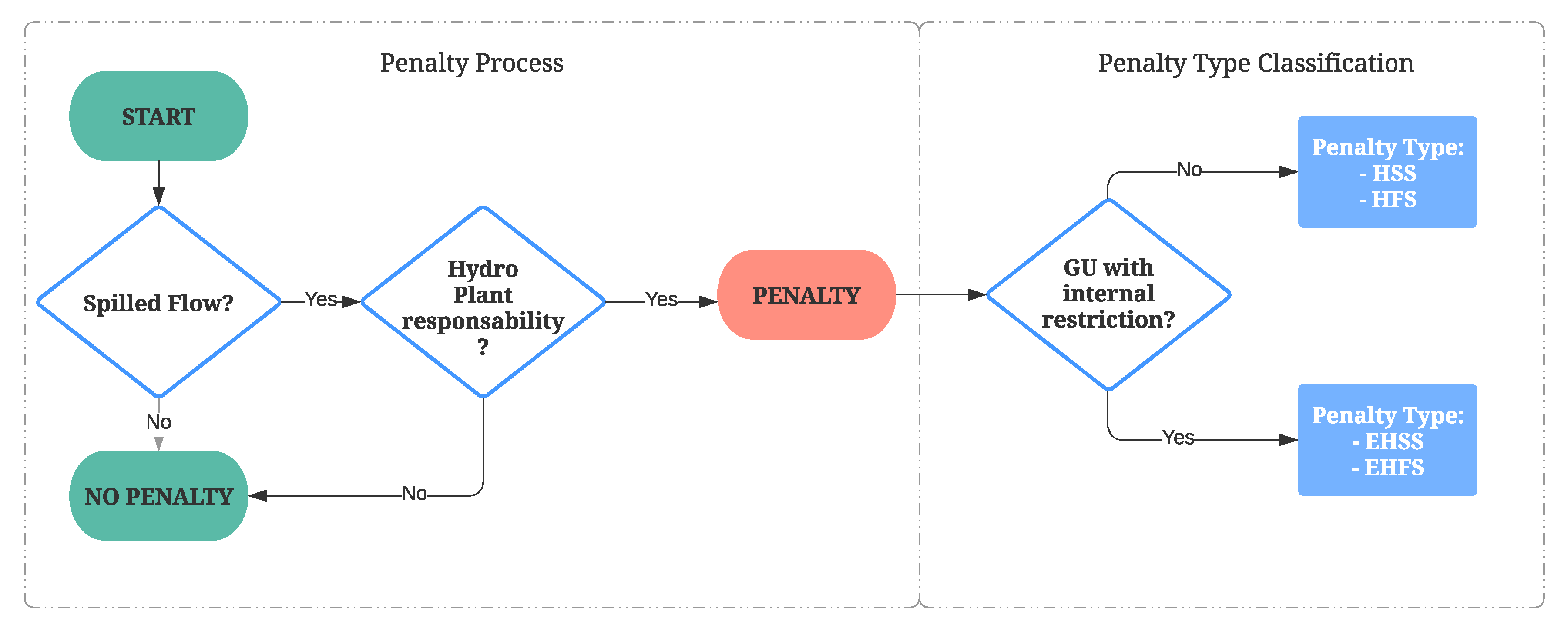
On the other hand, the flow subject to penalty, used in the Equation (
8), is calculated through the daily affluent flow (
) and the capacity of the plant. In certain periods of the year, the affluent flow is higher than the value that the plant can turbine, in which case, there will be a spillage that is not the responsibility of the plant, not penalizing it, as shown in the flowchart previously presented in
Figure 1. Therefore, through the Algorithm 1, it is possible to calculate the flow liable to be penalized.
| Algorithm 1: Algorithm for the Calculation of Penalty Affluent Flow. |
![Energies 14 08398 i001]() |
To optimize and allocate all maintenance, an iterative process is performed as shown in
Figure 2.
First, the maintenance is ordered from largest to smallest. Then, the first round of optimization is carried out, allocating and optimizing the largest duration maintenance for each GU. Next, the
m index is updated and the second round of optimization is performed. In this case, the restriction presented in the Equation (
11) is considered, limiting the possible days to allocate the start of the second largest maintenance of each GU. The process continues until the maximum number of necessary maintenances is met.
3.3. Monte Carlo Simulation
Monte Carlo Simulation is a statistical technique for predicting scenarios of future events by performing a series of probability computations. Thus, several simulations are carried out to cover most of the possibilities of occurrence of events [
26]. Monte Carlo Simulation makes a major contribution to risk analysis by building possible outcome models, calculating results continuously, each time using a different set of random values of the probability functions [
27].
In this work, random samplings related to forced shutdowns will be carried out for each GU in each month. Forced shutdowns are random and difficult to predict, in addition, they have great relevance in the context of hydroelectric plants, with a great impact on the operation of generating units, as well as financially influencing agents.
It is noteworthy that each generating unit has its particularities throughout the year, making it necessary to build probability curves and carry out monthly draws to better represent the reality of the hydroelectric plant. The parameters sampled in each MCS round for each GU in each month are:
The history used to obtain MCS input distributions comes from the SRCGU (System for the Register of Changes in the Operating States of Generating Units and International Interconnections), which is a database that records the forced and scheduled shutdown events of the hydroelectric plants in Brazil [
28]. In the database, the day of occurrence, the generating unit, the duration of the shutdown, and its type are informed. Therefore, it is a robust historical base that reflects the performance and behavior of the generating units.
After the sampling, the forced shutdowns will be inserted into an optimization model, which will calculate the plant’s operation, taking into account constructive aspects, forced and programmed restrictions. Then, the HFS indicator for the respective MCS scenario is calculated, which will be used in the sequence for the risk analysis. The MCS process runs until the established stopping criteria are met.
Figure 3 presents the general flowchart of the Monte Carlo Simulation proposed in this work.
3.3.1. Sampling the Random Variables
In this step, how the random variables were treated and sampled during the Monte Carlo Simulation will be described.
Number of Forced Event Days:
One of the most common techniques for modeling random behavior is through the Normal Distribution [
29]. The normal distribution is an absolutely continuous probability distribution parameterized by its mathematical expectation (real number
) and standard deviation (positive real number
).
In this case, for each generating unit in each month, a Normal Distribution (
) is obtained according to Equation (
16) through the history of shutdown hours (h) by forced constraint, where
and
represent the mean and standard deviation of the shutdown hours of unit
g in month
m.
With the distributions defined, the numbers of hours are sampled and the equivalent number of shutdown days for each GU in the month m is obtained.
Forced Events Occurrence Days:
With the number of shutdown days defined for the MCS round, the days in the month that the shutdowns will occur are sampled. Days of occurrence are modeled using a discrete distribution, which is a probability distribution that represents the occurrence of discrete and countable outcomes individually.
In this work, through the SRCGU database, 12 discrete distributions are obtained for each generating unit, one for each month of the year is created by counting the events that occur on each day of the month, that is, the days with more forced occurrences, they have a greater chance of being drawn.
Figure 4 shows the complete process for sampling the problem random variables, and it is important to highlight that the process is carried out for all GUs, observing the data for months separately.
In the following subsection, it will be presented how these days of the forced shutdown are worked to be inserted in the plant’s operation optimization modeling.
3.3.2. Operation Optimization
As previously mentioned, the forced shutdowns will be sampled at the MCS and inserted in a model to optimize the operation of the generating units. The optimal operation of the GUs considers the forced shutdown samples in the MCS and the maintenance calendar defined by the optimization in the Equations (
6)–(
14). Next, the plant availability indices regulated by NEEA will be calculated [
4].
Thus, an alteration to the previous model was implemented, including this random variable. Now, it is not necessary to optimize the maintenance schedule, but the plant’s operation in the face of forced and scheduled shutdowns. The impact of the randomness of this variable is evaluated using the MCS. In addition, in this work, the maintenance schedule is defined in advance, so the optimization will calculate the operation and spillage of the plant.
Again, the objective is to minimize the total spillage in the study horizon (Equation (
17)), by optimizing the operational state of each GU, considering the forced maintenance scenario generated during the MCS and the schedule of maintenance defined for the study horizon. Because the problem incorporates both binary and real variables, it is classified as a Mixed Integer Linear Problem (MILP). The proposed methodology for optimization in the scope of MCS is formulated by the Equations (
17)–(
23).
Optimization within the scope of the Monte Carlo Simulation receives the previously optimized maintenance schedule and the forced shutdowns drawn, directly impacting the operation of the generating units. Thus, through the matrices
and
it is possible to mathematically limit the operation due to programmed and forced shutdown, respectively.
Figure 5 presents an example of a
matrix construction.
The construction of is analogous to that of the matrix. In this case, the optimized shutdown days are entered into the matrix.
The Equations (
20) and (
21) have similar functions. In
and
each row represents a generating unit and each column a day, with each position being filled with 1 if there is the shutdown that day for the GU. As shown in Equation (
20), if
, its sum with
should be 1, in that case
is obligatorily 0, turning off the respective GU by programmed restriction. The same behavior occurs for
in Equation (
21), however the cause of the shutdown will be by forced restriction.
3.3.3. HFS Calculation
To understand the results and carry out an analysis of the impact of the forced shutdown at the plant, the availability indices referring to the HSS will be calculated in the same way as it is calculated in the AFA and described in the Equation (
24). The value of this indicator is found for each simulated scenario as seen in
Figure 3.
As mentioned, the AFA assesses the interruptions that occur due to maintenance, however, they are only accounted for when the NSO verifies spillage in the plant and this occurs under its responsibility [
23]. In this way, the numerator of the Equation (
24) only identifies the spill liable to be penalized. This value is divided by the average flow of the maximum turbined flow in each day
d. This ratio then finds the average number of GUs unavailable during that day due to forced interruption. Multiplying this value by 24 gives the number of hours of the forced shutdown that will impact the AFA.
It should be noted that in hydro plants, not all turbines are physically able to operate throughout the year, due to low flow, for example. Therefore, this particularity must be considered when calculating the average flow of the maximum turbined flow.
4. Case Study
The Santo Antônio Hydroelectric Power Plant (SAHP), located on the Madeira River in Porto Velho, Rondônia, Brazil, was chosen to address the case study. SAHP is a run-of-river plant, which means it has no regularization or storage capacity in its reservoir. It contains 50 Bulb GUs (24 with 4 blades and 26 with 5 blades) with a total installed capacity of 3568 MW and an assured energy capacity of 2424.20 MWmed [
30].
The values related to availability evaluated in the AFA calculation are registered in the NSO database through the SRCGU database. With this base, it was possible to identify the history of forced events that occurred in the hydroelectric plant, finding the average hours of interruptions for each GU in each month of the year and the period of occurrence recorded, information used in MCS.
The scheduled maintenance plan developed for the year 2021 by the maintenance team is found in
Table 1, where the total maintenance duration (MD) is in days and next to it is the number of maintenance required (MR) of the respective GU to meet the plan. This means that, for example, the U4-01 will be turned off to carry out preventive maintenance for 96 days a year, however, this shutdown will occur 4 times with different duration and that added up to the days, it will have ninety-six days.
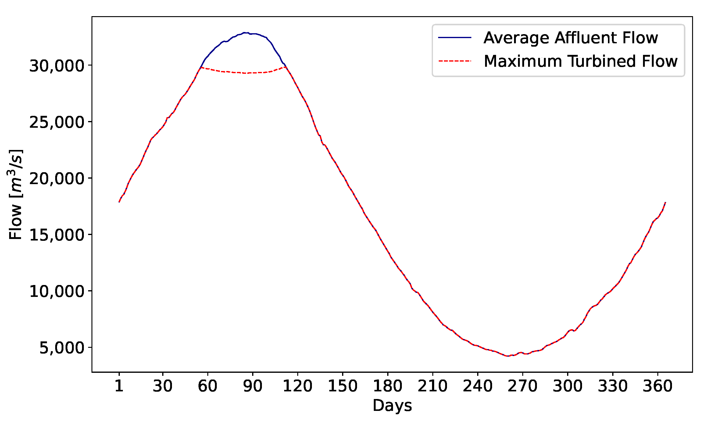
The SAHP’s affluent flow is significant data that should be assessed for GU maintenance planning. The low period in the case of SAHP is well characterized, as it is typical of the Madeira River, where the plant is located.
Figure 6 indicates the plant’s average affluent flow and the maximum turbined flow per day, which is the flow that can be penalized.
5. Results and Discussion
This chapter presents the results of the simulations proposed in this work. First, the result of the optimization presented in
Section 3.2 will be shown. Then, the result of two Monte Carlo simulations will be presented, the first using the history from 2017 to 2020 with the same weight. The second simulation, on the other hand, has a greater weight for the year 2020, as the objective is to verify what impact the improvements performed by the agent had on the risk analysis proposed by this work. The MCS stopping criteria is the max number of rounds, which is 10,000 for both simulations.
The simulations were performed using the Python language on the computer with the following configurations: Processor Intel
® Core
™ i5-7200U with 2.50 GHz and 16 GB of RAM, Linux version 5.11. In Python, equations are modeled using the Pyomo library [
31,
32]. The solver used is Gurobi, being one of the fastest and most powerful mathematical programming solvers available for multiple optimization problems [
33].
5.1. Maintenance Schedule Optimization
First, the optimization presented in the Equations (
6)–(
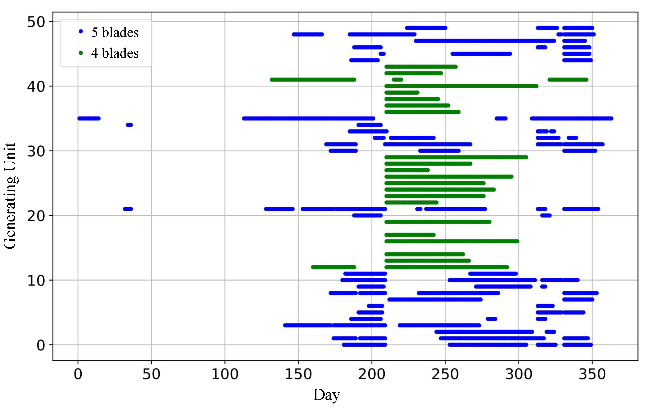
14) was performed, respecting the maintenance durations desired for the simulation horizon. The solution was found in 73.37 s (1 min and 13 s) with the maintenance calendar optimized as shown in
Figure 7.
All maintenance previously defined were allocated, respecting the continuity restriction. It is worth noting that the model tends to allocate maintenance in the low flow period, which occurs mainly after July. Therefore, after optimization, the PM matrix, derived from the maintenance schedule, can be built to be inserted in the MCS.
5.2. Simulation I
As presented in the previous sections, the proposed Monte Carlo Simulation was applied using parameters from SAHP. Probability curves for forced events are built with historical data from SRCGU and the maintenance schedule is defined by plant teams, daily over the year.
The rounds of MCS were performed to construct curves to observe the behavior of forced shutdowns in the year of study. First,
Figure 8 and
Figure 9 show curves related to the sum of HSS throughout the year.
In the Auction Notice n
005/2007, referring to the contracting of the Santo Antônio Energia HPP, it allows for a tolerance of 0.50% of HSS about the total number of hours of operation in the year, in this case, there are 438,000 total hours (50 GUs · 24 h · 365 days) of operation. Therefore, it is interesting to look at ranges of occurrence of HSS, providing the probability that each situation will occur.
Table 2 presents this analysis based on the proposed MCS.
Through the
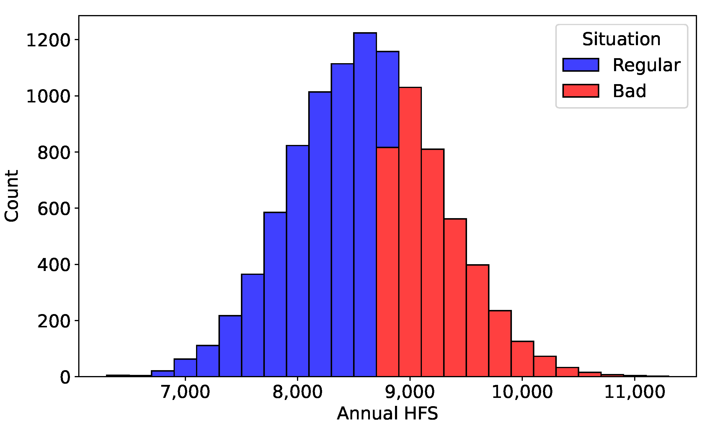
Table 2, it is observed that about 59% of the MCS scenarios result in a regular situation of plant operation. It is also worth mentioning that a considerable portion (approximately 41%) leads to a bad situation, serving as a warning for the plant, as it could lead to future critical situations.
Figure 10 complements the analysis, highlighting in the histogram the situations discussed in
Table 2.
In addition, it is important to emphasize that, according to the MCS proposed in this work, no scenario meets the conditions defined in the contract (HFS ≤ 2190.00 h), so with the simulation, it can be previously stated that the plant will be subject to penalties during the year of study.
5.3. Simulation II
The current state of the plant is different from previous years, as, over the years, the plant has taken corrective measures to minimize the hours of forced shutdowns in the generating units. Therefore, to quantify these improvements in the proposed MCS, the average for the year 2020 has a greater weight, thus, the present has a more significant impact without denying the influence of the past on the plant’s availability projections. It is noteworthy that the result found in
Section 5.1 is valid for Simulation I and II, as the maintenance calendar is optimized before the Monte Carlo Simulation and is not influenced by random sampling and their respective weights.
The second simulation allowed the agent to simulate an optimistic scenario since the model considered a higher probability of occurrence in the year 2020 (a scenario with a lower history of forced shutdown). As a result, the influence of pessimistic scenarios was minimized and the second simulation demonstrated the benefits of flexible models, enabling the extraction of multiple insights.
Therefore, in the second simulation, the mean () and standard deviation () are calculated with a higher weight for the 2020 values. The chosen weight was 50%, with the remainder equally distributed between the years 2017 to 2019. The main objective of Simulation II is to verify the improvement in the HFS indicator, validating the actions taken by the plant to obtain better performance.
The chosen 50% value was previously discussed by the researchers and SAHP engineers, since the objective of this weight is to represent as closely as possible the reality of interruptions in the following year (2021), given that improvements were implemented over the years and these effects were noticed in the year 2020.
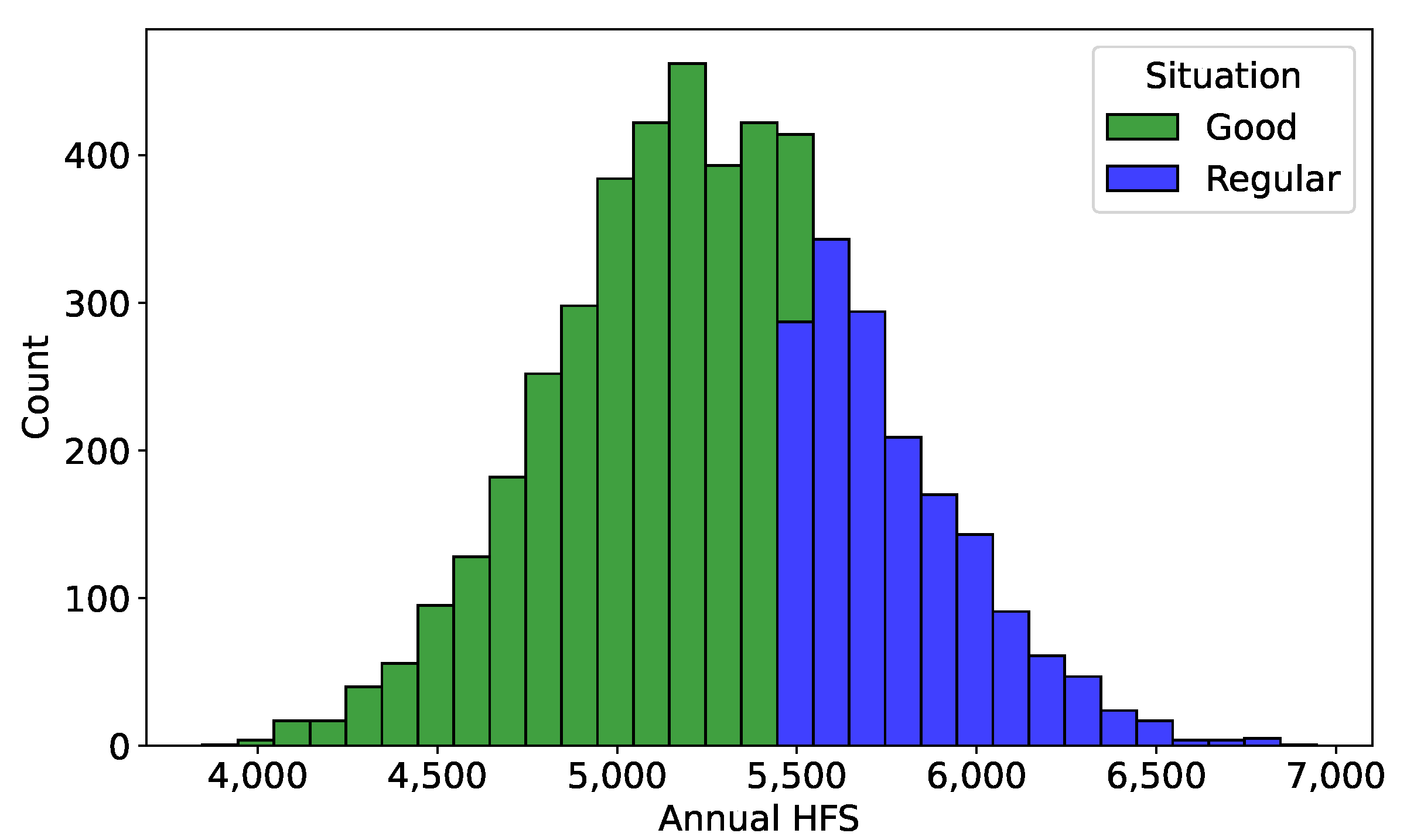
The best way to compare simulations is to look at the probabilities of HFS occurrence.
Figure 11 presents the MCS result for Simulation II, highlighting the occurrence ranges for each situation.
It can be seen in
Figure 11 a clear improvement in the plant’s performance, where 66% of the scenarios result in a good situation (2190 to 5475 h) and 34% in a regular situation (5475 to 8760 h). Remember that in Simulation I, the scenarios only result in a regular or bad situation.
Table 3 presents the ranges of occurrence of HFS for Simulation II.
Despite the reduction in future penalties, it is important to emphasize that even with the improvements, the plant will still be penalized, as no scenario results in an operation within the range allowed by the contract. Therefore, Simulation II shows that the agent is on the right path with the improvements made, which was possible to observe through
Figure 11 and
Table 3, however, the plant is still subject to penalties, and further improvements are needed to reduce the financial impact in the coming years.
6. Conclusions
This work presented a Monte Carlo Simulation to project the availability of hydroelectric plants. The proposed methodology addresses operational and regulatory aspects, where the plant’s availability is evaluated through the measured hours of interruptions due to scheduled and forced maintenance.
Therefore, the first point evaluated was about scheduled maintenance, developing an ideal maintenance schedule. This optimization considered regulatory aspects, as well as operational and duration restrictions and maintenance limitations, to minimize scheduled shutdown hours evaluated in the AFA, aiming to minimize financial penalties.
Regarding the portion of forced interruptions in the AFA, the MCS draws the hours of forced events, observing the history of measurements by SRCGU, calculated by the NSO. Thus, the methodology has a great regulatory framework, being of great importance for hydroelectric plants to assess their availability indices. The proposed methodology was simulated using real data from the Santo Antônio Hydroelectric Power Plant, with a simulation horizon of one year.
Through the results of the first simulation, it was possible to analyze the probability of occurrence of several HSS intervals in the year. The majority (approximately 59%) of the simulations resulted in a regular situation, however, it is worth noting that approximately 41% of the cases are in a bad situation, alerting the agent to possible critical operations. In addition, with MCS, it was possible to state that in the year of the study, the plant will be penalized, as it will violate the limit of hours defined by the contract.
The second simulation, on the other hand, demonstrates the flexibility of the model, allowing the agent to simulate pessimistic and optimistic scenarios, as is the case in this simulation. In this simulation, the model considered the probability of repeating the 2020 scenario greater and, therefore, the good scenario obtained the largest share.
Finally, the proposed model was successfully implemented using real data, achieving the goal of estimating the risk of regulatory penalties for the hydroelectric plant. In addition, the proposed methodology is applicable to other hydroelectric power plants.


 ,
, 


