2. RMS Simulation
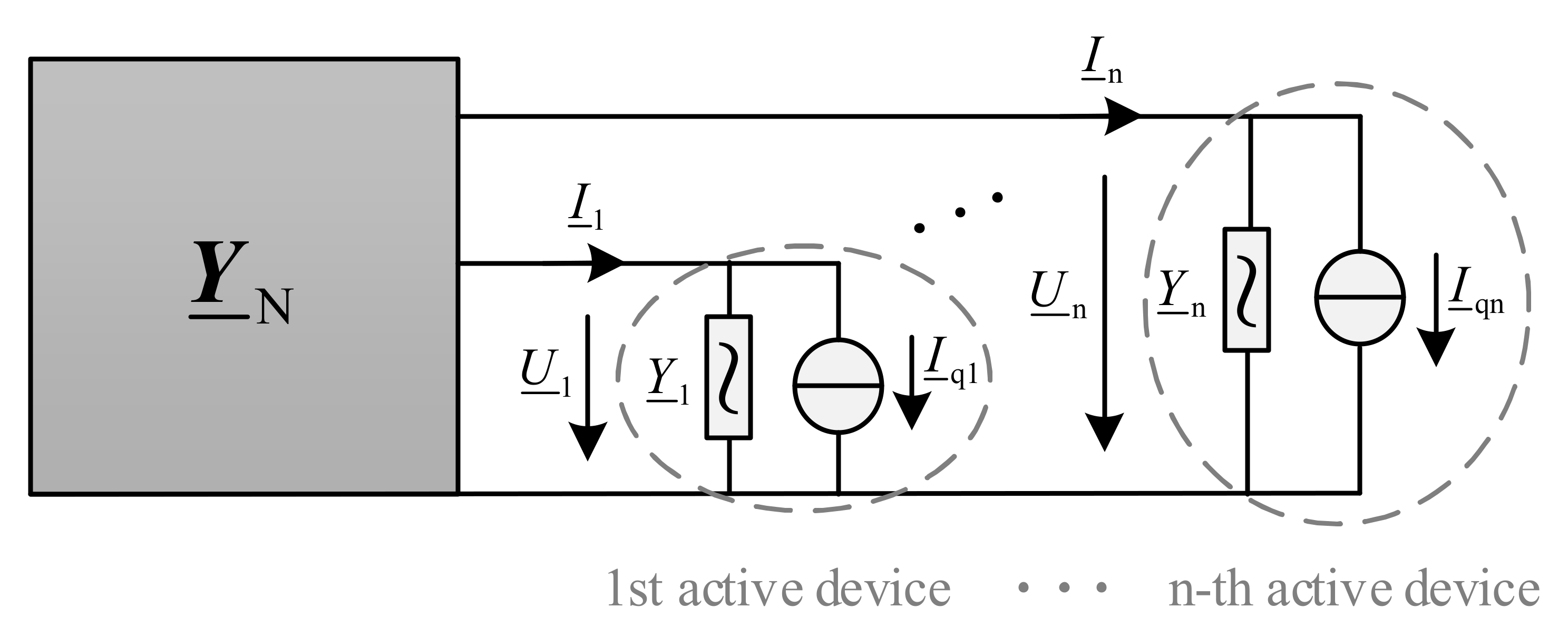
RMS simulation is used to analyze the long-term dynamic behavior of power systems. This simulation approach is based on the fact that fast electro-magnetic transients can be assumed to have already decayed in the time frame of interest, which allows higher time steps and therefore leads to lower simulation time comparing to EMT simulations. The models discussed in this paper are suitable for the investigation of balanced events in the network, and therefore only their positive sequence representations are taken into consideration. Equation (1) demonstrates the positive sequence of the overall network nodal equation system including
n nodes, whose associated visualization is illustrated in
Figure 1. The fundamental oscillation of voltages and currents is considered through their RMS values. Here as in the rest of the paper, the passive sign convention is chosen, so that consumed active and reactive powers are positive quantities. Furthermore, the equations are given on the principle of SI base units.
In RMS simulation, active devices (e.g., generating units and their respective control systems, dynamic loads, etc.) are considered by their quasi-steady-state models, whose dynamic behavior is represented by a set of differential equations, where the fast transients are neglected. As shown in
Figure 1, each active device is represented by its Norton equivalent circuit, whose current source depends on the state variables of the differential equations (
). The passive electrical network, which is considered by its steady-state model (i.e., a set of linear algebraic equations), connects the active device models. The right side of Equation (1) represents the matrix notation of the admittance equation of active devices, where
is a diagonal matrix whose diagonal elements are occupied by the internal admittances of the active devices. The left side of Equation (1) represents the passive electrical network, where the network admittance matrix
denotes the stationary model of the passive network, including the static loads. Furthermore,
,
and
represent the nodal voltage, nodal current and current source vectors. The resulting overall equation system constitutes an algebraic-differential equation system.
3. Wind Turbine Model
This section initially deals with all relevant sub-modules that are adopted in the same way in DFIG-based and FSC-based WT models, i.e., shared sub-modules. Afterwards, the special features of each WT model, consisting of their corresponding MSC controllers, are treated as the only model-specific sub-modules, and the few differences are highlighted. Finally, the transformation relationship between interface values of the WT model (space phasors) and the grid model (RMS values) is discussed. Furthermore, the linking of the converter models to the converter controller models is explained.
3.1. Shared Sub-Modules
The shared sub-modules of both WT models include the aerodynamic and drive train model, induction generator, pitch and speed controller and grid-side converter (GSC) controller, which are discussed in the following sections.
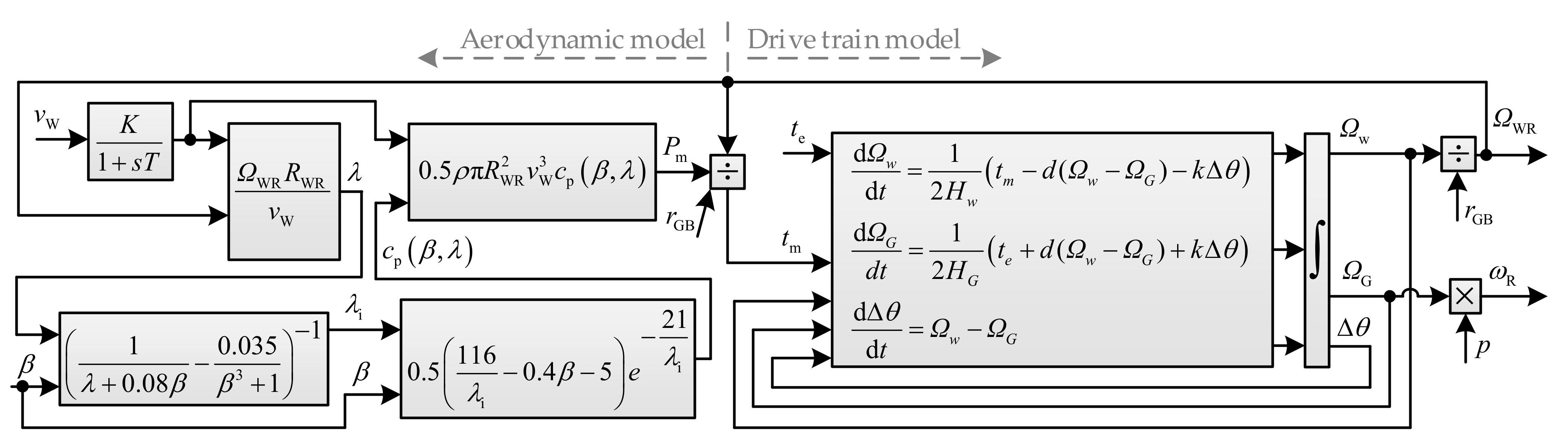
3.1.1. Aerodynamic and Drive Train Model
The aerodynamic behavior of the turbine rotor is modeled using the commonly applied approach, which is based on the aerodynamic power coefficient
as a function of the pitch angle
and the tip-speed ratio
[
6]. The mechanical torque
extracted from the wind is calculated using the block diagram of the aerodynamic model shown on the left side of
Figure 2. The model includes a low-pass filter, which ensures the smoothing of the high-frequency wind speed variations over the rotor surface [
4,
8,
18].
References [
19,
20] provide an overview of the drive train models of WTs with up to six distributed masses. Nevertheless, a two-mass model of the drive train is the commonly used representation, which properly considers the effect of torsional oscillations and therefore the dynamic impact of WTs on the grid [
12,
21,
22]. These effects have been noted in the literature for both WT models treated in this paper [
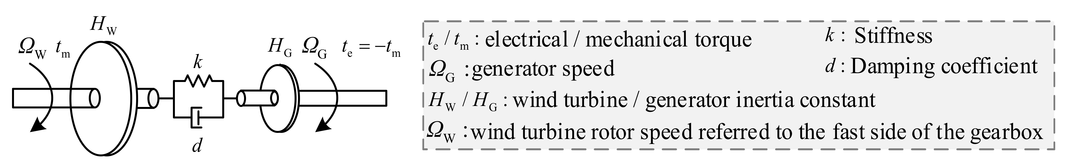
23]. Against this background, a two-mass mechanical model is applied in this paper, including a larger rotating mass representing the turbine inertia
and a smaller rotating mass representing the generator inertia
. The gear system is considered only as a transformation ratio
, since its inertia is negligible compared to the two other mentioned rotating masses.
Figure 3 shows the two-mass drive train model referring to the fast side of the gearbox.
The block diagram of the drive train model, including its differential equation system, is shown on the right side of
Figure 2, where
is the WT rotor speed and
is the generator speed considering the number of pole pairs.
3.1.2. Induction Generator
The following equation set (2)–(5) plus the equation of motion, which is considered in the equation system of the drive train model, represent the full-order model of an induction generator using space phasors [
9]. The equations are expressed in a rotating reference frame containing orthogonal direct (d) and quadrature (q) axes at the arbitrary stator angular frequency
, where the slip is defined as:
Due to the time frame of interest in RMS simulations, the fast stator transients are assumed to be already decayed within the time step of the simulation, as mentioned in
Section 2. Therefore, the derivative term in equation (2) is set to zero, i.e.,
[
9]. References [
21,
24,
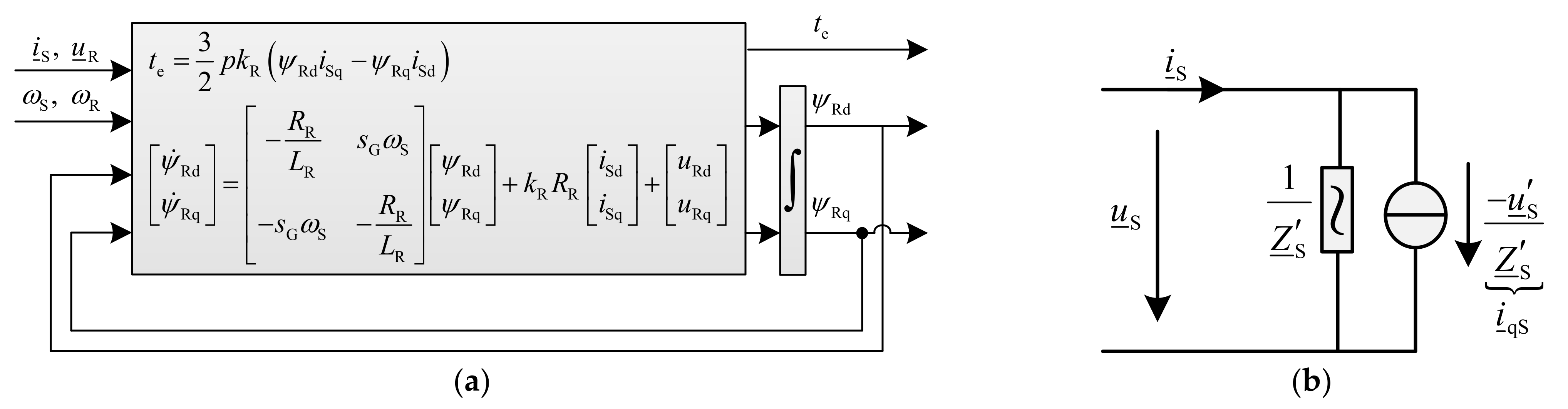
25] discuss the influence of the stator flux transients on the behavior of the WTs and confirm that they do not affect the long-term dynamic stability of the power system. Eliminating the rotor current in (4) using (5) and then substituting the stator flux linkage into (2) leads to Equation (6), which demonstrates the Thevenin equivalent circuit of the quasi-stationary (reduced-order) model, with
and
[
9]. Converting the Thevenin equivalent circuit to the Norton equivalent circuit leads to the circuit shown in
Figure 4b, which is integrable in Equation (1).
To calculate the transient voltage
and the electrical torque
, the differential equation of the rotor flux linkage needs to be solved. This equation is obtained by eliminating the rotor current in (3) using (5) and is shown in
Figure 4a separated into d- and q-components [
10].
3.1.3. Pitch and Speed Controller
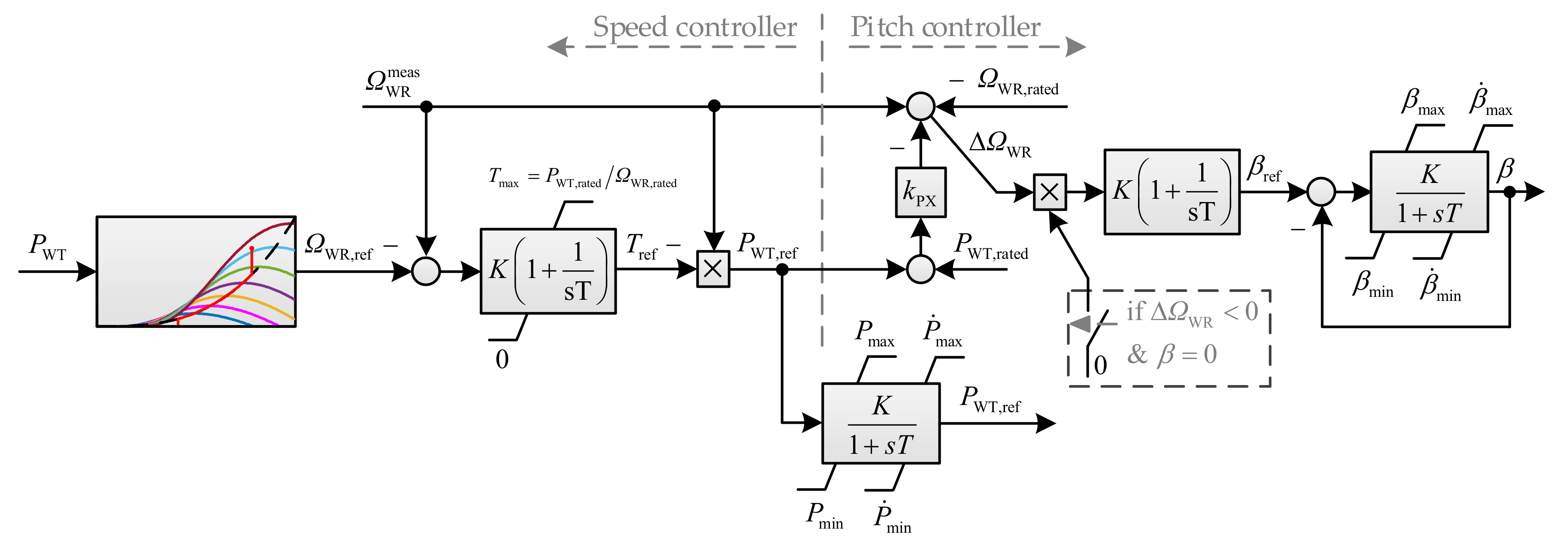
In order to extract the aerodynamically feasible optimal power from the wind under partial load conditions and feed it into the grid, the speed controller sets the WT rotor speed to an operating-point-specific optimal rotor speed according to a tracking characteristic curve. As depicted on the left side of
Figure 5, the speed controller simply consists of a PI controller, whose output signal is a torque reference value, and the input signal corresponds to the difference of the measured rotor speed and the rotor speed reference value provided by the tracking characteristic [
8]. Multiplication of the negative value of the torque signal with the measured rotor speed results in a power signal in the passive sign convention
, which serves as the power reference value of the MSC controller. The power set point is passed through a PT1 element to limit eventual power ramps [
26].
The commonly used control strategies of variable-speed WTs based on speed–torque or power–speed tracking characteristics are discussed in detail in [
3,
12,
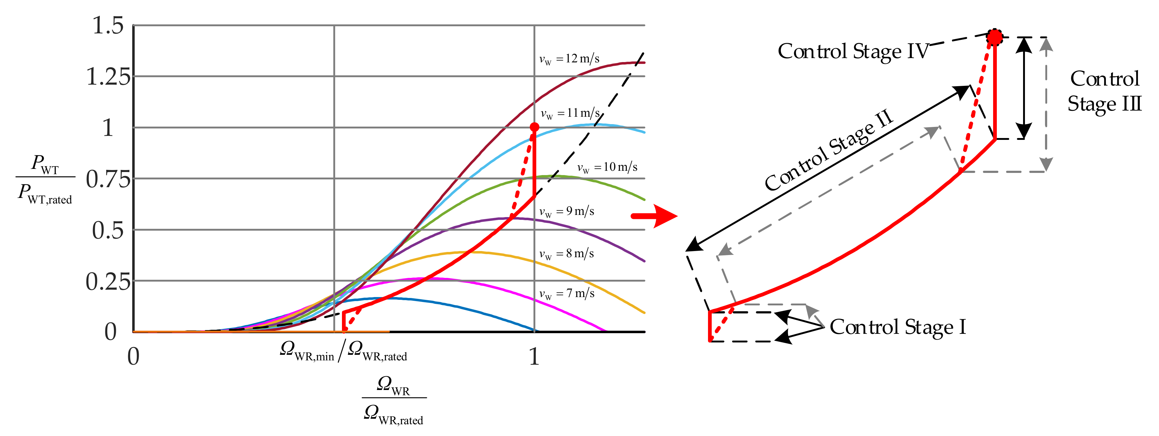
14]. The tracking curves are usually manufacturer-specific look-up tables, which are not necessarily known to researchers, and nevertheless they must be constructed based on available data in the literature. In this paper, a power–speed characteristic is designed based on the aerodynamic model of the rotor blades (see
Section 3.1.1.). The tracking characteristic curve is divided into four control stages, limited by three physical boundary values, i.e., minimum and rated rotor speed
and rated WT active power
, as shown in
Figure 6. The input value of the tracking characteristic block is the negative value of the measured terminal active power of the WT as a quantity in the passive sign convention. The output value is the reference rotor speed
, which results on the horizontal axis by tracking the solid red curve.
If the wind speed is in the range of the control stages I to III (i.e., below rated wind speed), the pitch angle is kept at optimum position of usually 0 deg and the speed controller adjusts the rotor speed
according to the solid red curve [
3]. The control stage I limits the rotor speed to a minimum value (
) and therefore prevents operating points, as the wind energy is not high enough to cover the electrical and mechanical losses of the turbine. At the variable-speed control stage II, in order to capture the maximum aerodynamically available power from the wind, the tip-speed ratio and thus the power coefficient are kept at their optimum values by tracking the optimum rotor speed. The optimum tip-speed ratio (
) is obtained by setting the first derivative of the power coefficient equation to zero, i.e.,
. The optimum power coefficient of the used aerodynamic model (see
Figure 2) is determined as
. The optimum tracking curve (the dashed black curve) can be constructed through Equation (7) to calculate the optimum rotor speed for the measured turbine output power in the corresponding operating point.
Once the rated rotor speed is reached (control stage III), the optimal tracking curve cannot be tracked anymore with increasing wind speed, and therefore the reference rotor speed is set to the rated rotor speed (
). The infinite gradient of the curve in this control stage may lead to large power fluctuations with small speed changes around the rated rotor speed. This consideration also applies to control stage I around the minimum rotor speed [
4]. To avoid these possible large power changes, the dashed red curve can be implemented instead of the solid red curve. The position of the connection points between control stage I and II and between II and III is a design decision [
4]. At the rated wind speed, the rated active power is also reached. At control stage IV, while the wind speed exceeds its rated value, the pitch controller consisting of a PI controller and a pitch actuator adjusts the rotor blade angle
by controlling the rotor speed, in order to affect the mechanical torque and consequently limit the power output to the rated power (
Figure 5). Since the WT operates already at the rated rotor speed, it is possible that the pitch controller becomes active before the rated power is reached. To avoid these undesired operating points, a signal consisting of the difference between the active power reference value and the rated active power is added, which produces a negative offset [
3]. The pitch actuator is modeled approximately as a PT1 element with pitch angle and ramp limitation.
3.1.4. Grid-Side Converter Controller
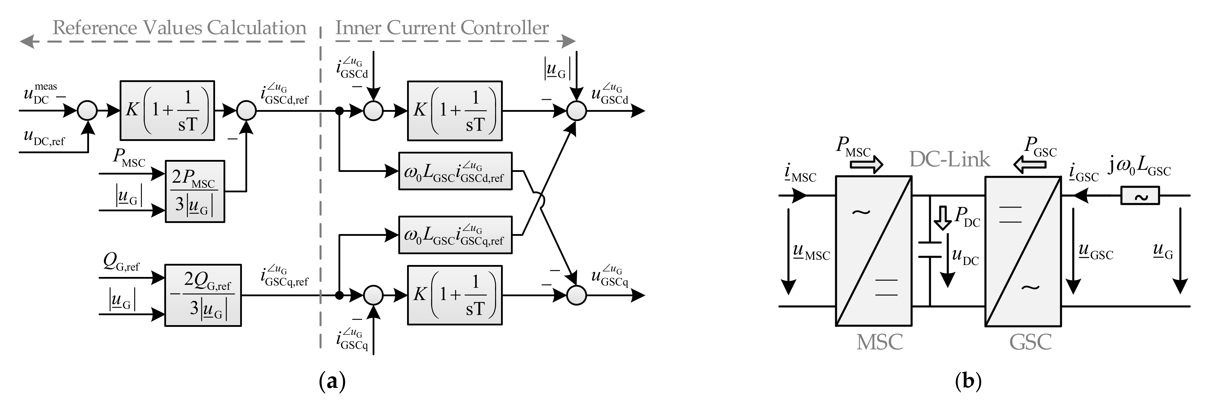
The first function of the GSC controller is to ensure the transition of the active power from the DC-link to the grid while maintaining the DC voltage. Furthermore, it can contribute to grid voltage support during steady-state and dynamic operation via reactive power provision. The control strategy is implemented utilizing a vector control approach based on current control in a dq-reference frame, which rotates with the network synchronous angular frequency
and is oriented to the terminal voltage of the GSC (
) [
8]. The orientation of the dq-reference frame to the terminal voltage ensures a decoupled control of active and reactive current and is denoted by the superscript
. The following space phasor equation describes the voltage of the GSC according to the grid side of
Figure 7b.
After separation of Equation (8) into d- and q-components and replacement of the term
with PI controllers, the inner current controller can be derived, as illustrated on the right side of
Figure 7a. The d-component of the GSC current (
) corresponds to the active current, while its q-component (
) corresponds to the negative of the reactive current. Based on the power balance equation at the DC node by neglecting the converter losses (Equation (10)) and considering the apparent power equation at the GSC terminals in the voltage-oriented reference frame (Equation (9)), current reference values of the d- and q-components can be obtained, as shown on the left side of
Figure 7a. The DC voltage control is implemented by replacing the term
with a PI controller. In order to counteract the effect of parameter and measurement inaccuracies, PI controllers are needed to ensure a precise control [
8].
While the MSC active power is provided by the rotor circuit of DFIG (
), the reactive power reference value
can be provided by a power factor, reactive power or voltage controller. In each time step, the DC voltage is calculated by integrating the result of Equation (11), which is derived from the current equation at the DC node.
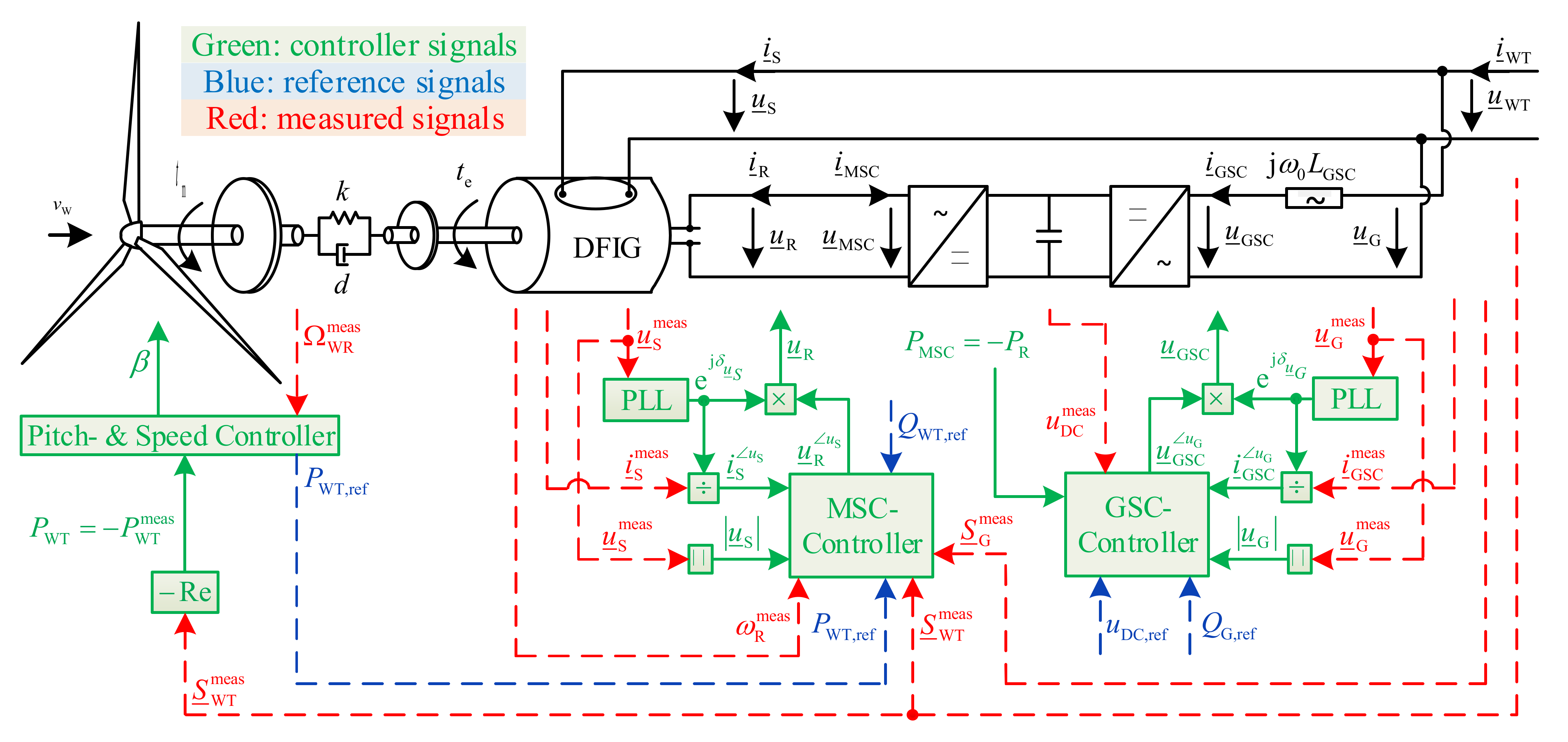
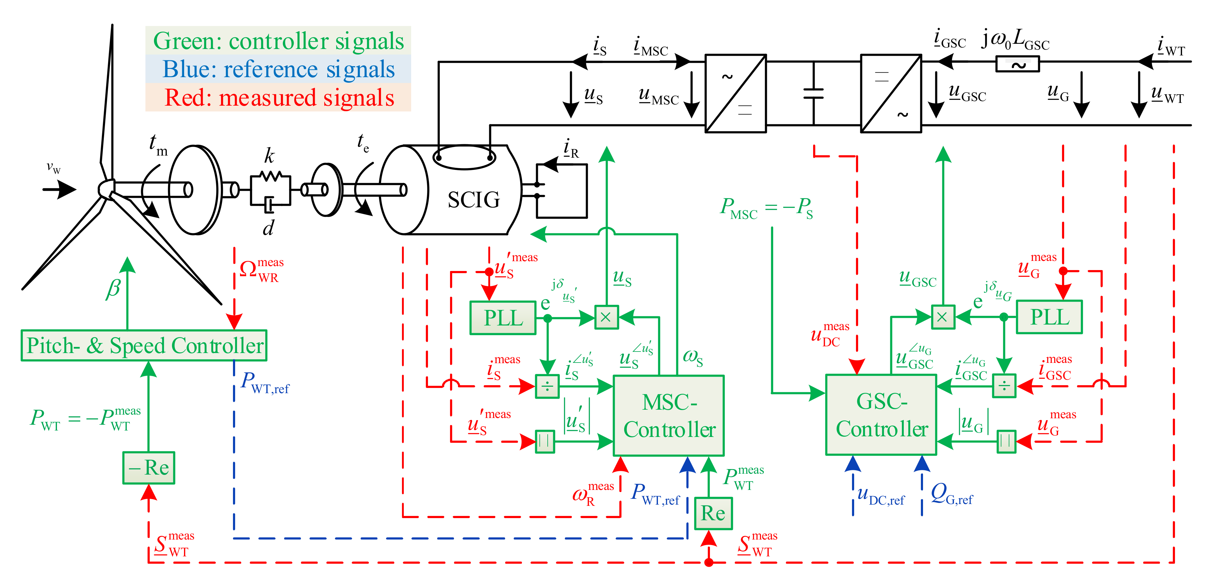
3.2. Special Features of Doubly Fed Induction-Generator-Based Wind Turbine
The overall control system of a variable-speed WT based on DFIG is illustrated in
Figure 8. All sub-modules explained in
Section 3.1 are implemented in the same way. The only difference is that in the equations of the wound rotor induction generator from
Section 3.1.2, the stator angular frequency
is expediently replaced by the grid synchronous angular frequency
, since the stator terminals of the DFIG are directly coupled to the grid. This means that the dq-reference frame of the DFIG equation system is assumed to rotate synchronously with the grid reference frame. As shown in
Figure 8, the rotor terminals are connected to the grid via a back-to-back frequency converter consisting of two independently controlled voltage source converters (MSC and GSC), which are rated for a fraction of the total generator power (slip power
), where
is the air-gap power. The amount and the direction of the power fed into the grid via the rotor circuit depends on the generator speed (power flow from the generator to the grid in sub-synchronous operating points and vice versa in super-synchronous operating points in the passive sign convention). The MSC controller is the only model-specific sub-module, which is described in the following section.
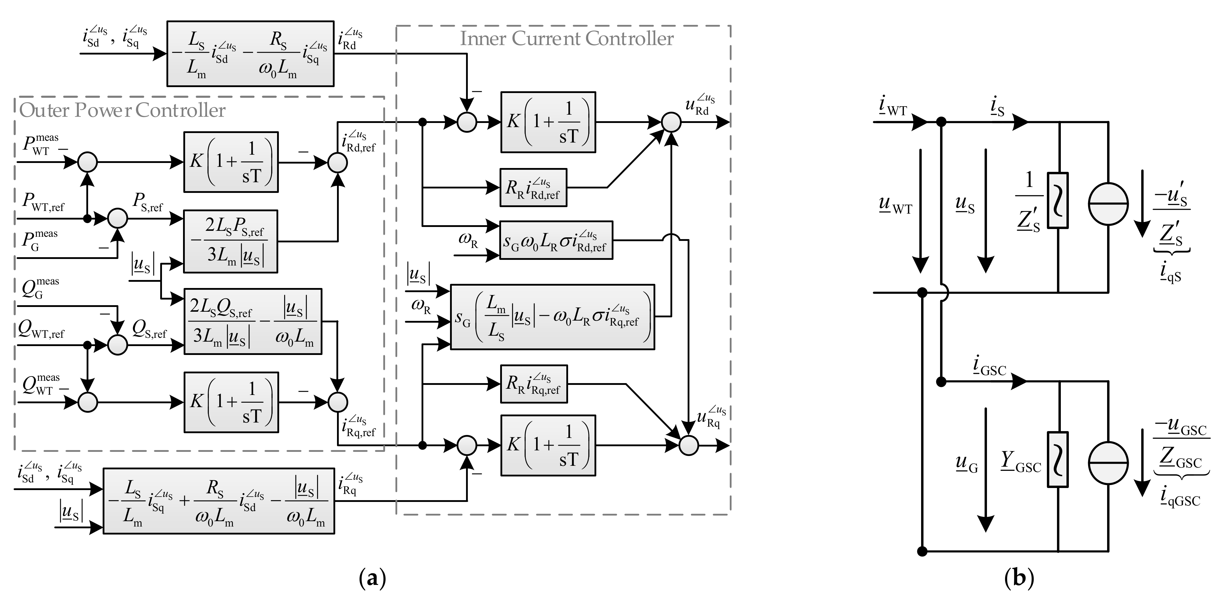
Machine-Side Converter Controller
The function of the MSC controller is the independent control of the active and reactive power at the measurement grid point (i.e., the WT terminals), which is realized through rotor current control. The MSC control approach applied in this paper is designed based on the control concepts presented in [
8,
13]. The MSC control strategy has a cascade structure, which contains a faster (inner) rotor current control loop to calculate the impressed rotor voltage and a slower (outer) power control loop to determine the rotor current reference values. The different time constants of the two control loops are due to the fact that the electrical dynamic responses of the converters and the DFIG are much faster than the mechanical dynamic response of the turbine. They serve to avoid undesired controller interactions and ensure controller stability. The control objective of the MSC controller can be achieved utilizing a vector control approach in a stator-voltage-oriented dq-reference frame and feeding the rotor terminals with a voltage of variable frequency and amplitude. The principle of deriving the stator voltage orientation of the dq-reference frame from the field-oriented control (stator flux orientation) as a common practice in electrical drives is explained in detail in [
13].
The structure of the MSC controller is based on the stationary form of the machine equation system, setting
. Thus, to derive the rotor voltage equation as a function of controlled and measured values (
and
), the derivative terms of Equations (2)–(5) are neglected (
,
). Furthermore, these equations are transformed into the stator-voltage-oriented dq-reference frame, where
. The superscript
indicates the stator-voltage-orientated reference frame. Eliminating the stator flux linkage in Equation (2) using Equation (4) and its subsequent rearranging to obtain
results in the following equation.
Substituting (12) into (5) and then eliminating the rotor flux linkage in (3) through the obtained equation results in Equation (13). In this equation, the stator resistance is neglected,
and
.
The alignment of the reference frame with the stator voltage and the projection of currents on this reference frame enable an independent control of active and reactive current, so that changes in the d-component () lead to active power change, while changes in the q-component () lead to reactive power change.
Separation of Equation (13) into d- and q-components and extension of the resulting equations with PI controllers in order to fully compensate for the control error lead to the control structure of the decoupled inner current controller, as illustrated in
Figure 9a. The rotor current can be calculated by rearranging Equation (12). The power control loop consists of a direct calculation of the rotor current reference values based on the generator model, which enhances and speeds up the dynamic performance. The rotor current reference value can be obtained by rearranging Equation (12) and replacing the stator current components with the stator active and reactive power reference values, whereby the stator resistance is omitted (
), as shown in Equation (15). Equation (14) shows the stator active and reactive power reference values as functions of the stator current reference values.
While the active power reference value is calculated by the speed controller (see
Section 3.1.3), the reactive power reference value is provided by the wind park controller. Equation (14) is extended by PI controllers to improve the steady-state accuracy of the power control loop, which is shown in
Figure 9a. Interconnecting of the DFIG equivalent circuit shown in
Figure 4b and the Norton equivalent circuit of GSC leads to the overall Norton equivalent circuit of the DFIG-based WT (
Figure 9b), which is now integrable in the network nodal equation system (Equation (1)).
3.3. Special Features of Full-Scale-Converter-Based Wind Turbine
The overall control system of the variable-speed FSC-based WT is illustrated in
Figure 10. As shown in the figure, the stator terminals are connected to the grid via a back-to-back frequency converter consisting of two separately controlled voltage source converters (MSC and GSC). As a result, the entire power of the generator is fed into the grid via the frequency converter, which results in a higher rated power compared to converters of DFIG-based WTs. While the MSC is intended to control the dynamic behavior of the generator, the GSC is supposed to ensure compliance with the grid requirements. This leads to a fully controlled current injection of the FSC-based WTs according to the programmed behavior of the converter, in contrast to the DFIG-based WTs, whose behavior is a combination of controlled behavior of the converter and inherent behavior of the induction generator.
As the induction generator is fully decoupled from the grid via the DC-link of the frequency converter, there is no reactive power exchange between the generator and the grid. As a result, the reactive current of the generator is provided by the MSC. To reduce the demand for reactive power generation by the MSC and therefore reduce the power rating of the MSC, fixed capacitors can be applied at the generator terminals. Thus, the MSC only needs to be rated to supply the lacking excitation reactive power in high-load operation and to absorb its surplus in low-load operation in order to prevent over-excitation of the generator [
27].
Similar to the DFIG-based WT, all sub-modules explained in
Section 3.1 are implemented in the same way except for the MSC controller that is introduced in the following section. Furthermore, the rotor voltage
in the machine equations of
Section 3.1.2 is set to zero (squirrel-cage induction generator SCIG), which is why the slip power
is wasted as rotor losses in the rotor circuit (
).
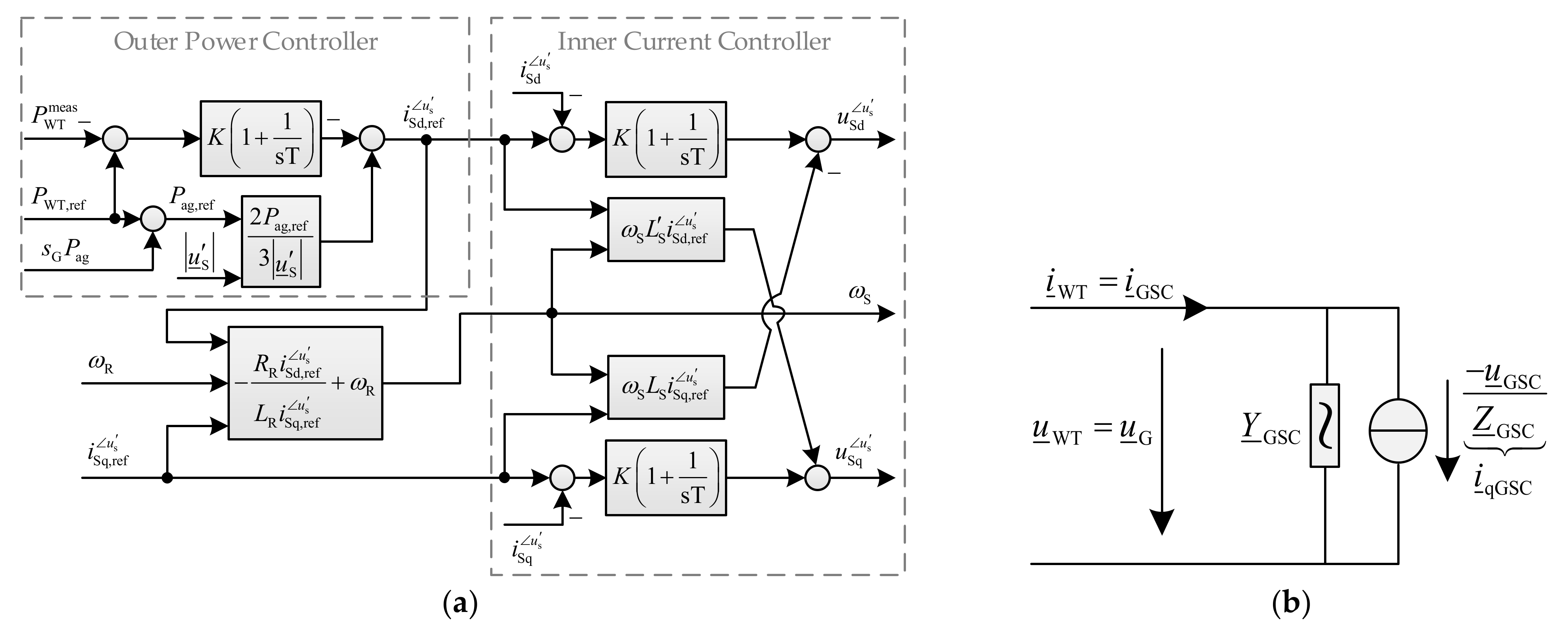
Machine-Side Converter Controller
The function of an MSC controller is to control the active power output of a WT according to the optimization of the power extracted from incoming wind, which is realized through stator current control. The control objective of the MSC controller can be achieved utilizing a vector control approach in a transient-voltage-oriented dq-reference frame and feeding the stator terminals with a voltage of variable frequency and amplitude. Reference [
5] describes the MSC control approach based on a rotor-flux-linkage-oriented reference frame. The motivation for using the transient-voltage-oriented reference frame in this paper is the control it provides of WT active power output according to the power reference value from the speed controller based on the tracking characteristic curve (see
Figure 5). Furthermore, it is intended to provide an analogy to the MSC control approach of the DFIG-based WT. Since the structure of the MSC controller is based on the stationary form of the induction machine equation system, the derivative terms of rotor and stator flux linkage are neglected in the following (
,
).
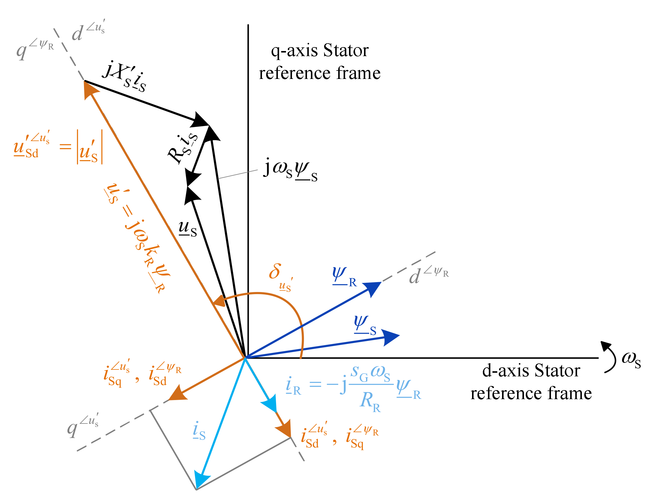
Figure 11 shows the phasor diagram of the SCIG for an assumed operating point in the stator dq-reference frame. Furthermore, the transient-voltage-oriented reference frame and its relation to the well-known field-oriented (rotor-flux-oriented) reference frame is depicted.
The projection of the stator current on the transient-voltage-oriented reference frame shows that the d-component
is responsible for the active power control (torque control) according to Equation (23) and the q-component
contributes to the rotor flux linkage according to Equation (18). The influence of the stator current components in the rotor-flux-linkage-oriented reference frame is opposite, since this coordinate system lags the transient-voltage-oriented reference frame by 90 degrees (see
Figure 11). The MSC control strategy has a cascade structure, which contains an inner stator current control loop to calculate the impressed stator voltage and an outer power control loop to determine the d-component of the stator current reference value. Since the induction generator is operated in the constant flux region, as described in [
5], the q-component of the stator current is controlled at a constant value, which is provided by the initialization procedure (see
Section 4.2). To derive the stator voltage equation as a function of the controlled value (
), the stationary machine Equations (2)–(5) are considered below, neglecting the stator resistance (
) and setting
. As a consequence of the alignment of the reference frame to the transient voltage (
), Equation (6) will have the following form:
The superscript
indicates the orientation of the reference
frame to the transient voltage. After rearranging Equation (3) under
consideration of
and
to calculate the slip frequency
and adding it to the rotor angular frequency
, the equation of the stator angular frequency
is obtained (Equation (17)). The phasors of the equation are already transformed into the transient-voltage-oriented reference frame, where the rotor current solely consists of its d-component and the rotor flux linkage is represented by its q-component (
,
), as illustrated in
Figure 11.
To obtain the d-component of the rotor current and the q-component of the rotor flux linkage as functions of the stator current components, Equation (5) is transformed into the transient-voltage-oriented reference frame. Equations (18) and (19) express the resulting equation separated into d- and q-components.
Eliminating the rotor current and rotor flux linkage in Equation (17) using Equations (18) and (19) results in the following equation.
Under consideration of Equations (6) and (18), the absolute value of the transient voltage can be expressed depending on the stator current as the controlled variable:
Substituting Equation (21) in Equation (16) leads to the stator voltage equation as a function of stator current. Separation of this equation into d- and q-components and extension of the resulting equations with PI controllers in order to fully compensate the control error lead to the control structure of the inner current controller, as illustrated on the right side of
Figure 12a. The power control loop consists of a direct calculation of the d-component of the stator current reference value based on the air-gap power equation (Equation (22)), which enhances and speeds up the dynamic performance.
The d-component of the stator current reference value in the transient-voltage-oriented reference frame can be obtained by rearranging Equation (22) considering
:
As illustrated on the left side of
Figure 12a, Equation (23) is extended by a PI controller, whose power reference value is supplied by the speed controller to improve the steady-state accuracy of the power control loop. Since all sub-modules of the FSC-based WT except the GSC are fully decoupled from the grid via the DC-link of the frequency converter, the FSC-based WT model is represented in the network nodal equation system (Equation (1)) by the Norton equivalent circuit of its GSC (
Figure 12b).
3.4. Model Interfacing
3.4.1. Wind Turbine Models—Grid Model
The positive sequence grid model is represented through stationary RMS values of currents and voltages in a synchronously rotating coordinate system (i.e., with nominal electrical angular frequency
). The sub-modules of WT models with an interface to the grid, i.e., DFIG and GSC of both models, are expediently described using space phasors in a reference frame rotating synchronously with
. In order to clarify the connection between the sub-modules mentioned above and the grid model, the transformation relationship between their interface values (RMS values and space phasors) is illustrated in the following equation [
10]:
is the initial angle between the real axes of both coordinate systems, which is assumed to be zero in this paper (
). As mentioned in
Section 2, the WT models, as active components, are also represented in the network overall equation system by their Norton equivalent circuits, as shown in
Figure 9b and
Figure 12b. In each time step of the simulation, the space phasors of the source currents are known from the numerical integration of the generator differential equations and the output values of the GSC controller transformed into the synchronously rotating grid coordinate system. After calculation of their RMS values (
,
) according to Equation (25), the RMS values of the stator and GSC terminal voltages (
,
), along with all other network node voltages, can be calculated by rearranging Equation (1), as demonstrated in Equation (26).
The RMS values of the stator and the GSC terminal currents (
and
) can now be calculated according to the left side of Equation (1). The space phasors of these terminal voltages and currents, which are denoted in
Figure 8 and
Figure 10 as measured values, are calculated through Equation (24).
3.4.2. Converter Models-Converter Controller Models
As shown in
Figure 8 and
Figure 10, the transformation of the interface variables of the converters (measured voltages and currents) into the voltage-oriented coordinate systems of the converter controllers is carried out by dividing them by
,
or
. The transformation in other direction is done by multiplying them by these terms. In RMS simulations, the angle of the RMS value of the GSC terminal voltage
can be directly considered as the orientation angle of the GSC controller, while the angle of the RMS value of the stator terminal voltage
is the orientation angle of the MSC controller in the DFIG-based WT model. The transformation angle of the MSC controller in the FSC-based WT model
is the angle of the rotor flux linkage, which is measurable in the induction generator model, shifted by 90 degrees, as shown in
Figure 11. In order to determine the orientation angles in the RMS simulation, so-called phase-locked loops (PLLs) can be modelled with a sufficient accuracy as a PT1 element [
26].
4. Initialization
The objective of the initialization procedure is to calculate the initial values of the internal variables and the state variables of all sub-modules explained in the previous sections based on a stationary state of the network, which results from a power flow calculation. In large-scale dynamic simulations containing a high number of WTs, an appropriate initialization procedure is extremely important to avoid undesired electrical transients and possible numerical instabilities at the beginning of the simulations. Furthermore, an inaccurate initialization may result in a major discrepancy between the initialization and the power flow outcome. This leads to a different stationary state of the network after damping of transients and possibly to an incorrect evaluation of the dynamic performance of the power system. In the following sections, the initialization procedures of both WT models are addressed. They are based on the power–speed characteristic described in
Section 3.1.3 and a steady-state model of the induction generator, which is implemented as DFIG or SCIG. In both cases, the terminal voltage
and the apparent power of the WT
are known from the power flow calculation and the procedure is based on the same active power equation of the WT (Equation (28)).
Since the structures of the speed, GSC and MSC controllers are derived from the stationary equations of the induction generator and GSC, their initial values will also be obtained from the initialization of the induction generator and GSC. Due to the presupposition of a stationary network state, all time derivatives in the differential equations are set to zero. The reference values of all PI controllers and PT1 elements are equal to their actual values. As a result, the input signals of PI controllers become zero, and their state variables can generally be calculated as follow:
The WTs are assumed to be at partial load operation points, and thus the pitch angle is set to zero, so there is no need to initialize the pitch controller.
4.1. DFIG-Based Wind Turbine
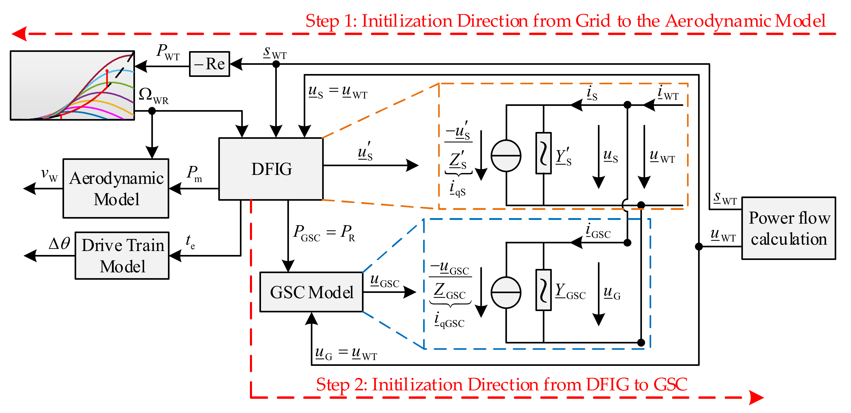
The initialization procedure of the DFIG-based WT used in this paper is divided into two successive initialization steps, as illustrated in
Figure 13. The first step starts with the initialization of the DFIG, the aerodynamic and the drive train model based on the results of a power flow calculation and the power–speed characteristic. The second step consists of the initialization of the GSC based on the rotor power obtained in the first step.
4.1.1. DFIG
The initialization of the DFIG model is performed based on the following active power equation of the WT in the passive sign convention, while neglecting the converter losses:
The d-component of the stator current can be calculated using Equation (29).
Elimination of the rotor flux linkage and rotor current components as well as the d-component of the stator current in Equation (28) using Equation (5), Equation (6) and Equation (29) leads to Equation (30) as a function of
, where the constant values
and
are as follows:
The rotor angular frequency
and therefore the slip
are known according to the power–speed tracking characteristic. The reactive power reference value of the GSC (
) is predefined, which is usually set to zero in steady-state operation. Furthermore, and as mentioned above, the terminal voltage of the induction generator (
) and the active and reactive power of the WT (
) are known from the power flow calculation. The quadratic Equation (30) has two solutions. The solution with the smaller absolute value is selected as the q-component of the stator current. The d-component of the stator current can be calculated using Equation (29). The transient voltage
and thus the electrical state variables of the DFIG (
,
) can be determined using Equation (6). The electrical torque
, the rotor current
and the rotor voltage
can be determined considering the torque equation in
Figure 4a, Equation (5) and the stationary form of Equation (3).
4.1.2. Aerodynamic and Drive Train Model
The input values of the initialization procedure of the aerodynamic model are the rotor speed
, which is known according to the power–speed tracking characteristic and the initial mechanical power calculated from the already determined electrical values of the induction generator, i.e.,
. The initial wind speed along the control stage II of the tracking characteristic curve can be calculated with sufficient accuracy using the following equation:
The initial wind speed along the control stage III should be calculated iteratively. At the beginning of the iteration procedure, Equation (31) provides a sufficiently precise starting value for the wind speed. The goal of the iteration procedure is that the mechanical power calculated from wind speed, rotor speed and power coefficient corresponds to the initial mechanical power
mentioned above. At each iteration step, the wind speed is increased, and consequently the power coefficient and the mechanical power are recalculated using the aerodynamic model (the left side of
Figure 2) until the following iteration condition is fulfilled.
Considering the stationary form of the drive train model equation system depicted in
Figure 2, the shaft twist angle is the only variable that must be initialized as:
4.1.3. GSC
Since a stationary operating point is assumed during the initialization procedure, there is a power balance at the DC node, i.e., there is no energy exchange with the DC link capacitor (
). Consequently, the GSC active power is equal to the negative MSC active power and can be calculated from the already determined rotor variables:
Furthermore, the terminal voltage
is known from the power flow calculation, and the reactive power of the GSC is a predefined reference value (
). The current
can be calculated using the apparent power equation at the GSC terminals. Finally, the GSC voltage
can be calculated according to the Kirchhoff’s voltage law in the grid side of the
Figure 7b. The initialization of the GSC controller is carried out in a terminal-voltage-oriented reference frame.
4.2. FSC-Based Wind Turbine
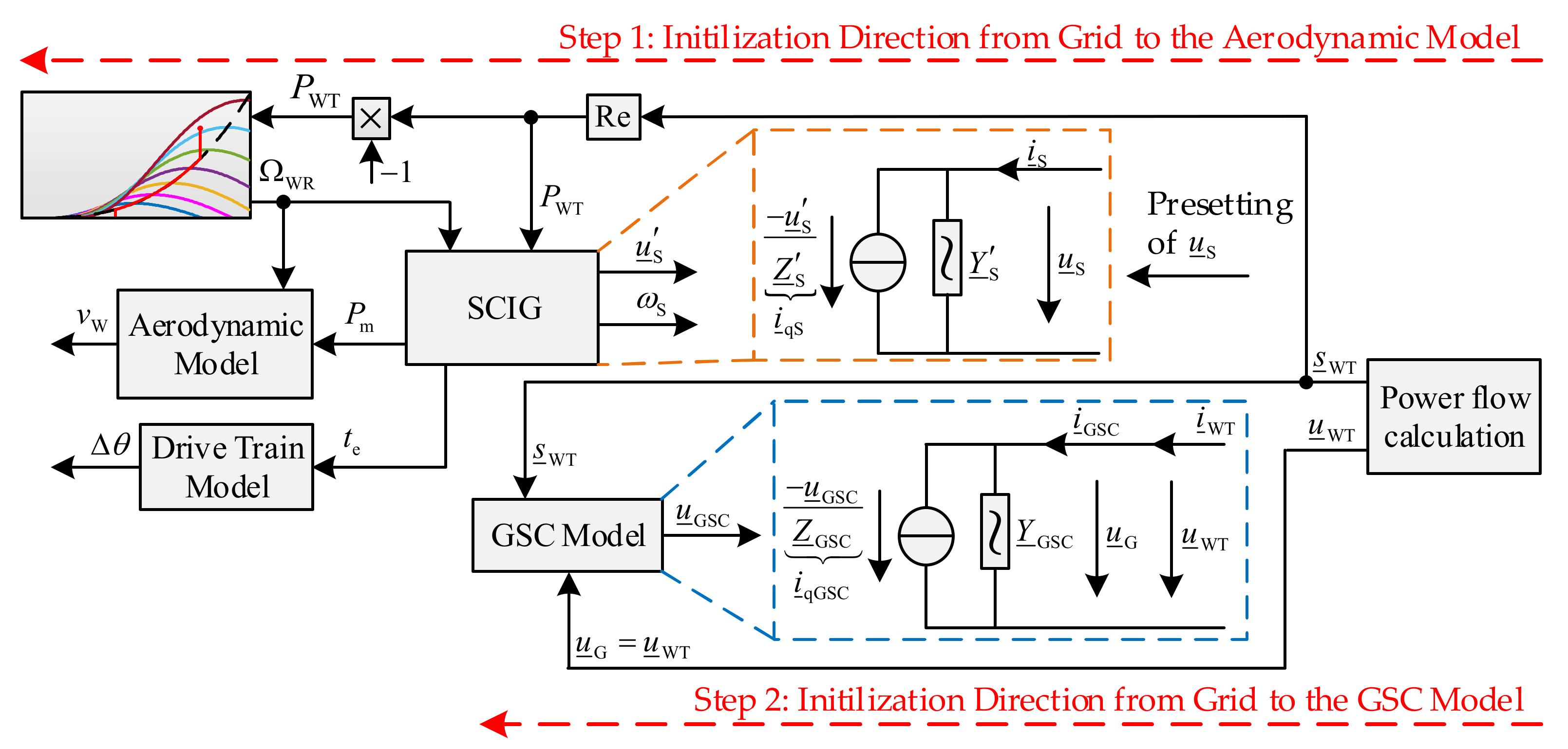
The initialization procedure of the FSC-based WT used in this paper is also divided into two initialization steps, as illustrated in
Figure 14. The first step deals with the initialization of the SCIG, the aerodynamic and the drive train model based on the results of a power flow calculation and the power–speed characteristic. The second step consists of the initialization of the GSC, which is also based on the results of a power flow calculation. Since the GSC is decoupled from the other sub-components of the WT model by the DC link, the initialization steps can be executed independently.
4.2.1. SCIG
The initialization of the SCIG model, as with that of the DFIG model, is performed based on the active power equation of the WT (Equation (28)). Since the reactive power demand of the machine is unknown, Equation (29) cannot be taken into account. In contrast to DFIG model, the stator angular frequency
in the SCIG model is an unknown variable. To eliminate the rotor flux linkage, rotor current and stator current components in Equation (28) and obtain an final equation as a function of stator angular frequency (Equation (35)), the stationary form of the rotor flux linkage equation system (
Figure 4a) for a SCIG (
), Equations (5) and (6) are applied, where
.
The rotor angular frequency
and the active power of the WT
are known from the power–speed tracking characteristic and the power flow calculation. In order to solve the equation, the stator voltage
should be preset as the actuating variable of the MSC controller. This quartic equation has four solutions. The complex solutions are excluded. Furthermore, the solution with the smallest difference to the rotor angular frequency
is selected. Once
is calculated, the d- and q-component of the stator current can be determined using Equations (36) and (37). These equations are obtained by eliminating the rotor flux linkage in Equation (6) using the stationary form of the rotor flux linkage equations. Thus, the transient voltage, the rotor flux linkage and the electric torque can be determined considering Equation (6) and
Figure 4a.
4.2.2. Aerodynamic and Drive Train Model
The initialization procedures of the aerodynamic and drive train model described in
Section 4.1.2. can be applied in the same way.
4.2.3. GSC
The initialization procedure of the GSC model described in
Section 4.1.3. can be applied in the same way. The only difference is that the GSC active power
does not need to be calculated but is equal to the WT terminal active power, which is known from the power flow calculation.
5. Fast Frequency Response
In the event of a sudden frequency drop due to an imbalance between generation and demand in a power system, the directly grid-connected synchronous generators of the conventional power plants contribute to the system inertia by inherently releasing the kinetic energy stored in their rotating mass in order to maintain the frequency stability indicators (i.e., rate of change of frequency (ROCOF) and frequency nadir (FN)) within predefined thresholds. The continuously increasing penetration of power electronic-interfaced generating units (PEGU) leads to a reduction in the overall system inertia as an essential parameter for frequency stability [
28], which consequently has a negative effect on both ROCOF and FN. Therefore, as a countermeasure, the network code for requirements for grid connection of generators sets requirements for capability of power park modules (PPMs) to provide synthetic inertia (SI) to replace the effect of inertia on a synchronous power-generating module to a prescribed level of performance [
29]. Another alternative solution to improve the frequency performance of the power system with a high-level penetration of PEGU during contingencies is referred to as FFR or fast active power injection (FAPI). In [
28], FFR is defined as a reaction of PPMs in the very first seconds of a frequency drop by quickly activating the active power contribution to counteract the effects of low system inertia.
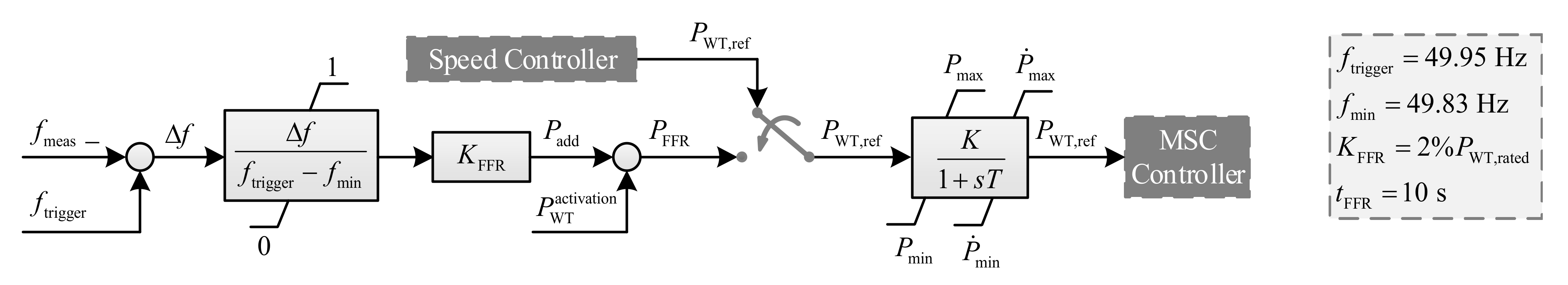
The frequency response controller implemented in this paper is the ENERCON IE control system [
30], which is a droop-based system that reacts to a grid frequency below a predefined trigger threshold by temporarily increasing the active power (see
Figure 15). The additional energy to cover this power raise
is extracted from the rotating mass of the WT as a result of its deceleration.
Since this control system does not provide a response proportional to ROCOF, it cannot deliver an inherent frequency response like a synchronous generator, often termed “true inertial response”, and thus it falls into the FFR category rather than SI. As illustrated in
Figure 15, in FFR mode, the speed controller is deactivated, and the active power set point of the MSC controller is supplied by the FFR controller for a preset time window
. The input signal of the FFR controller corresponds to the deviation of measured frequency
from the trigger frequency
. The output signal represents the sum of the WT active power output at the time of FFR activation
and an additional power signal
that exhibits the following linear dependency on the frequency deviation:
The value of the gain
can be set as a proportion of WT rated active power. According to Equation (38),
is the maximum possible additional power that is fully commanded when the measured frequency reaches the minimum frequency limit
. The controller parameters chosen in this paper are shown on the right side of
Figure 15. As the measured frequency rises back above the trigger frequency
or the activation time period
has expired, the FFR mode is deactivated, and the active power set point of the MSC controller is supplied by the speed controller again. The speed controller, including its PT1 element, then provides a smooth re-acceleration of the WT to the operating point prior to the FFR activation on the tracking characteristic curve. A smooth recovery phase with a limited power reduction ensures that the power system does not realize the re-acceleration of the WTs as a second frequency drop [
30].
6. Case Study
The simulation results presented in this chapter serve primarily as examples to demonstrate the initialization performance and the general operation of the WT models at different operating points, taking into account a set of step responses to different deterministic wind speeds. Furthermore, the functionality of the WT models equipped with the above-mentioned FFR controller is illustrated and briefly discussed. Neither a parameter analysis and tuning nor a performance assessment of the FFR capability is intended. In order to execute the first example simulations, the 2 MW DFIG-based and FSC-based WT models are coupled to a 20 kV passive equivalent grid via a transformer (0.69/20 kV). The model parameters of both WT models used in the case studies are identical and can be found in [
8].
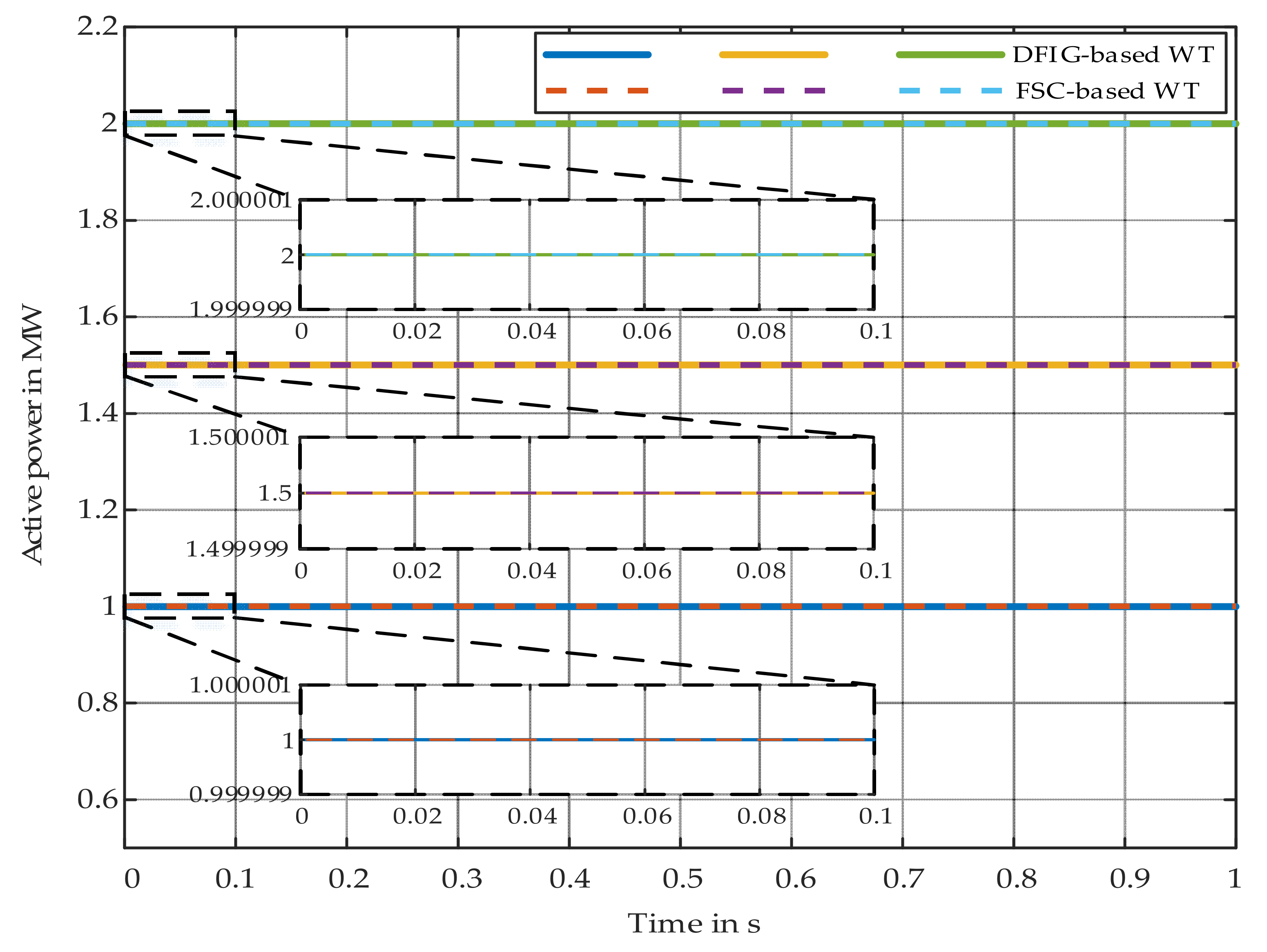
Figure 16 shows exemplarily the active power output of both WT models for three different stationary operating points.
The straight lines prove that the results of the introduced initialization procedures match the power flow calculation results with a very high accuracy at each examined operating point.
Figure 17 and
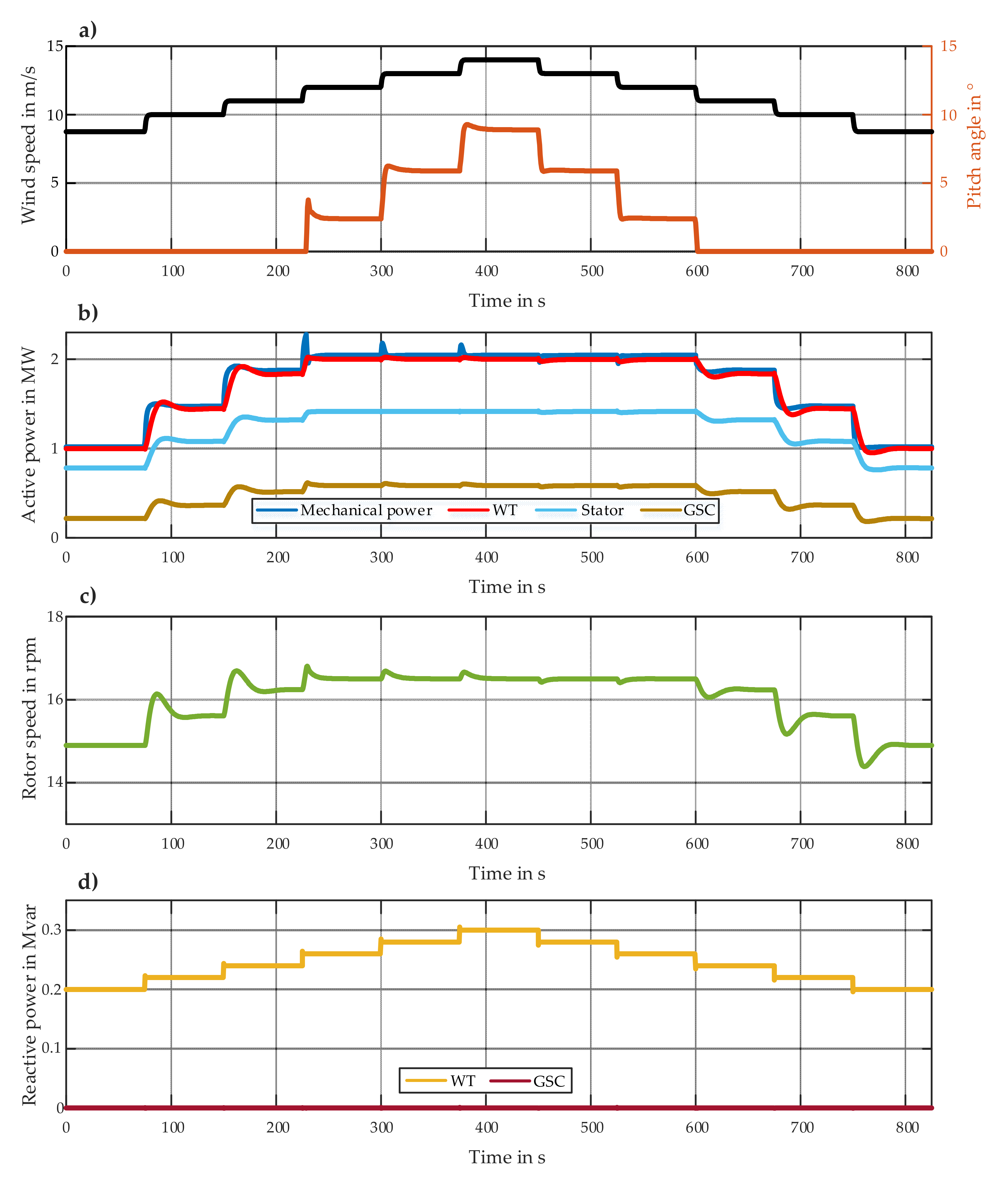
Figure 18 show some characteristic variables of step response simulations of both WT models.
The initial operating point in each case is based on terminal output apparent power of 1 MW + j0.2 Mvar, which is determined from a Newton–Raphson-based power flow calculation [
10]. The initial wind speed of each simulation is 8.7 m/s, which is calculated using Equation (31). In the first part of both simulations, the wind speed is increased from the initial value to 10 m/s and then to 14 m/s, with 1 m/s steps every 75 s (
Figure 17a and
Figure 18a). Furthermore, the WT reactive power reference value is increased from the initial value to 0.3 Mvar with 0.02 Mvar steps, as shown in
Figure 17d and
Figure 18d. In the second part, the operating points return to the initial values with the same step sizes. At wind speeds lower than 12 m/s, the speed controller controls the rotor speed according to the tracking characteristic curve (
Figure 17c and
Figure 18c). The MSC controller controls the WT terminal active power to its reference value provided by the speed controller. At wind speeds equal to or higher than 12 m/s, the pitch controller adjusts the rotor blade angle by controlling the rotor speed and limits the mechanical torque and consequently the output active power to the WT rated power (
Figure 17b and
Figure 18b). The output active power of the FSC-based WT is equal to the stator active power and the GSC active power neglecting the converter losses. Its output reactive power is equal to the GSC reactive power. The output active and reactive power of the DFIG-based WT is composed of the stator portion and the GSC portion. The reactive power of the GSC is kept at zero over the whole simulation time.
In order to demonstrate the contribution of the WT models to improving the frequency performance of power systems, the WT models are implemented in a MATLAB-based RMS simulation tool, which is discussed in [
15,
16] and is referred to as a “distributed-rotating-mass based model”. Synchronous generators in this simulation tool are modelled using a fifth-order state space model commonly called model 2.1, according to the IEEE Std 1110-2002 [
31]. The excitation systems are represented by a ST1C excitation system with a PSS1A stabilizer from the IEEE Std 421.5-2016 [
32]. The implemented generic model of prime movers and their control systems, which are also discussed in [
15], enable the simulation of secondary and primary control power activation in accordance with the specific regulatory requirements [
33,
34]. The used composite load model consists of a dynamic component (i.e., a third-order induction motor) and a static component, which is referred to as ZIP model [
35]. The passive network components (i.e., transformers and transmission lines) are represented by their steady-state models. The model parameters of all devices and their corresponding controllers used in the following scenarios can be found in [
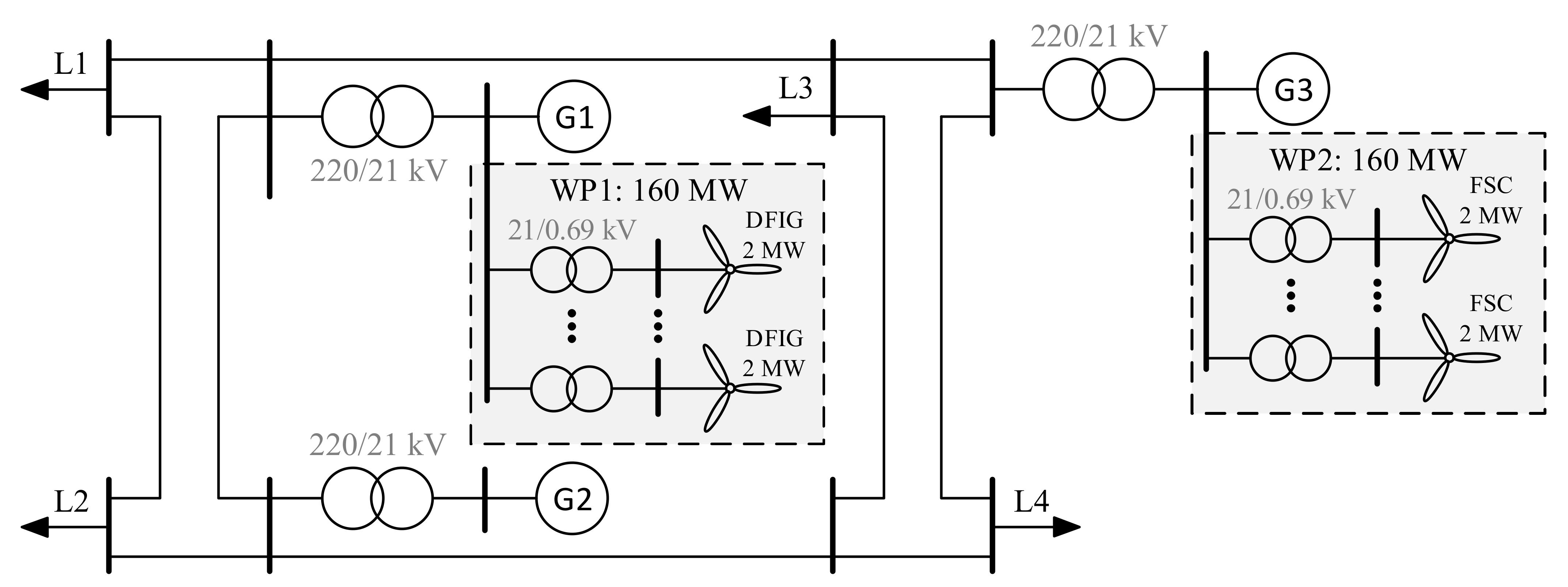
16]. The single line diagram depicted in
Figure 19 shows the topology of a 220 kV test system. Three synchronous generators (G) and two wind parks (WP) feed four loads (L) via the transmission grid. WP1 consists of 80 DFIG-based WTs and WP2 is composed of 80 FSC-based WTs. Each WT has a rated active power of 2 MW. No aggregation of the WT models is performed in this paper.
Table 3 shows the initial terminal apparent powers of the synchronous generators, loads and wind power plants prior to the disturbance resulted from a Newton–Raphson-based power flow calculation [
10].
Two scenarios with constant wind speed are simulated based on an unscheduled increase in load L1 by 45 MW after 60 s. In the first scenario, the FFR controllers of all WTs are deactivated. Thus, only the synchronous generators offer their inertia to control the ROCOF and the frequency nadir. In the second scenario, fifty percent of the WTs in each WP provide FFR capabilities.
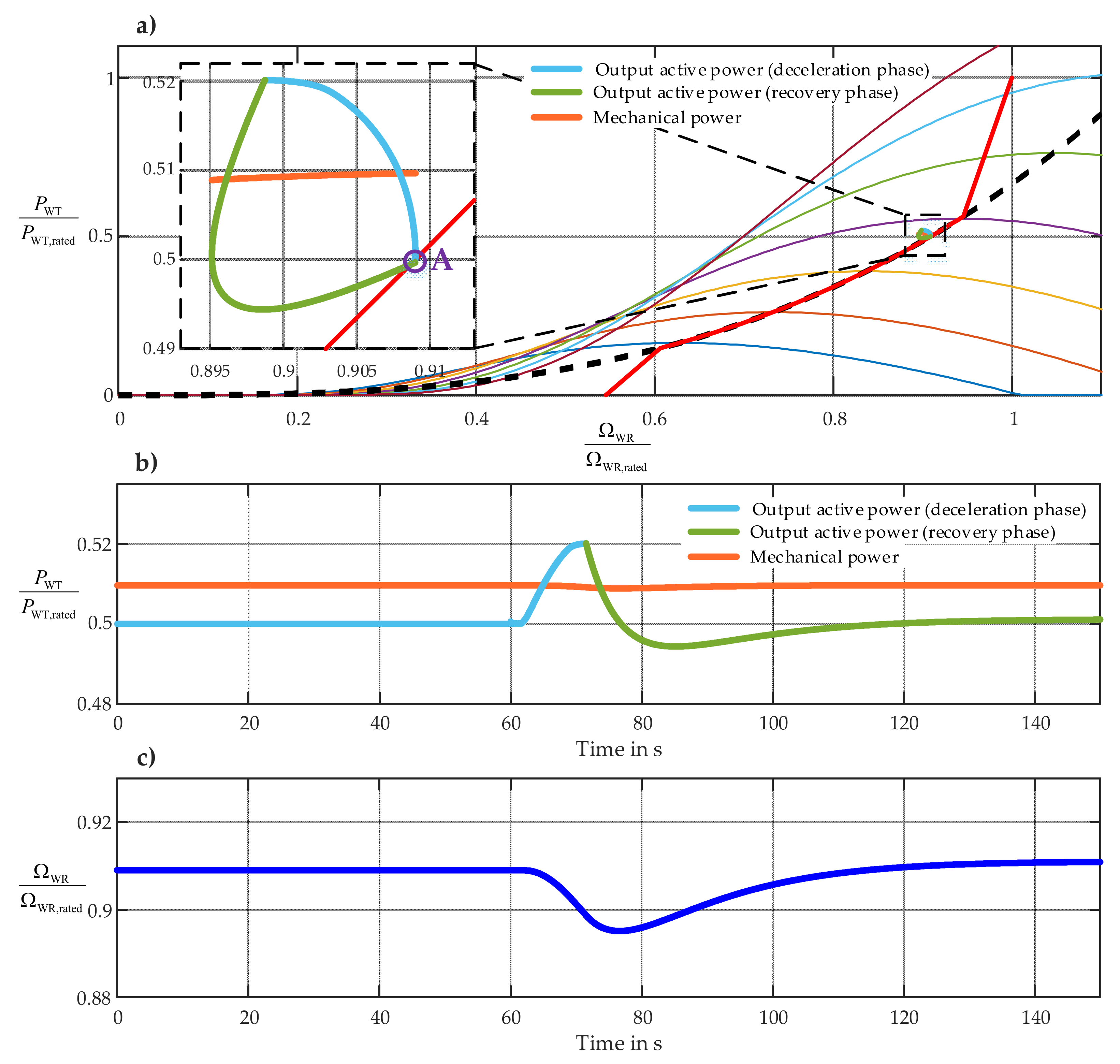
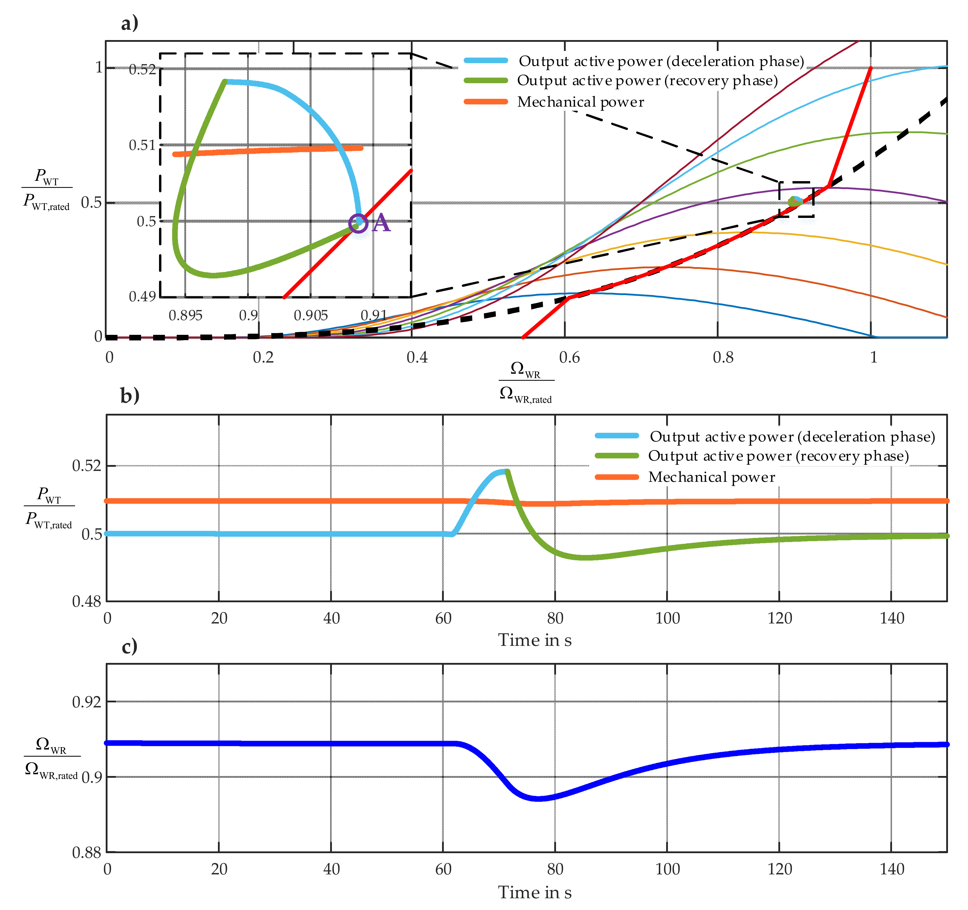
Figure 20a and
Figure 21a demonstrate the power and rotor speed response of an exemplary DFIG-based WT from WP1 and an exemplary FSC-based WT from WP2, respectively, to the above-mentioned disturbance in the second scenario by means of power–speed characteristic curve. A very similar behavior of both WT models can be observed. Point A in each figure represents the stationary operating point before the perturbation. After the grid frequency reaches the threshold and the FFR controller is triggered, the sum of the WT active power output at the time of FFR activation
and the predefined additional power signal
is commanded to the MSC controller as the active power set point. In the overproduction phase (i.e., the light blue curve), since the electrical output power plus the WT losses is higher than the available mechanical power extracted from the wind, the rotating mass of the WT decelerates, and the rotor speed decreases. The slope of the light blue curve can be modified by setting the minimum frequency limit
. The higher this frequency is set, the steeper the light blue curve becomes. If the activation time period
is elapsed, the speed controller will be activated, and the recovery phase (i.e., the light green curve) starts with the aim of re-accelerating of the WT to the desired operating point on the tracking characteristic curve, which depends on the actual wind speed. Since the wind speed is constant during this scenario, the desired rotor speed is the pre-fault rotor speed (i.e., point A).
Figure 20b,c and
Figure 21b,c show the mechanical power, the output active power and the WT rotor speed of both selected WTs in the overproduction phase and the recovery phase in time domain. The first 60 s of the curves in time domain show the illustrated variables in the pre-fault time window, which again confirm very well-functioning initialization procedures of both WT-models.
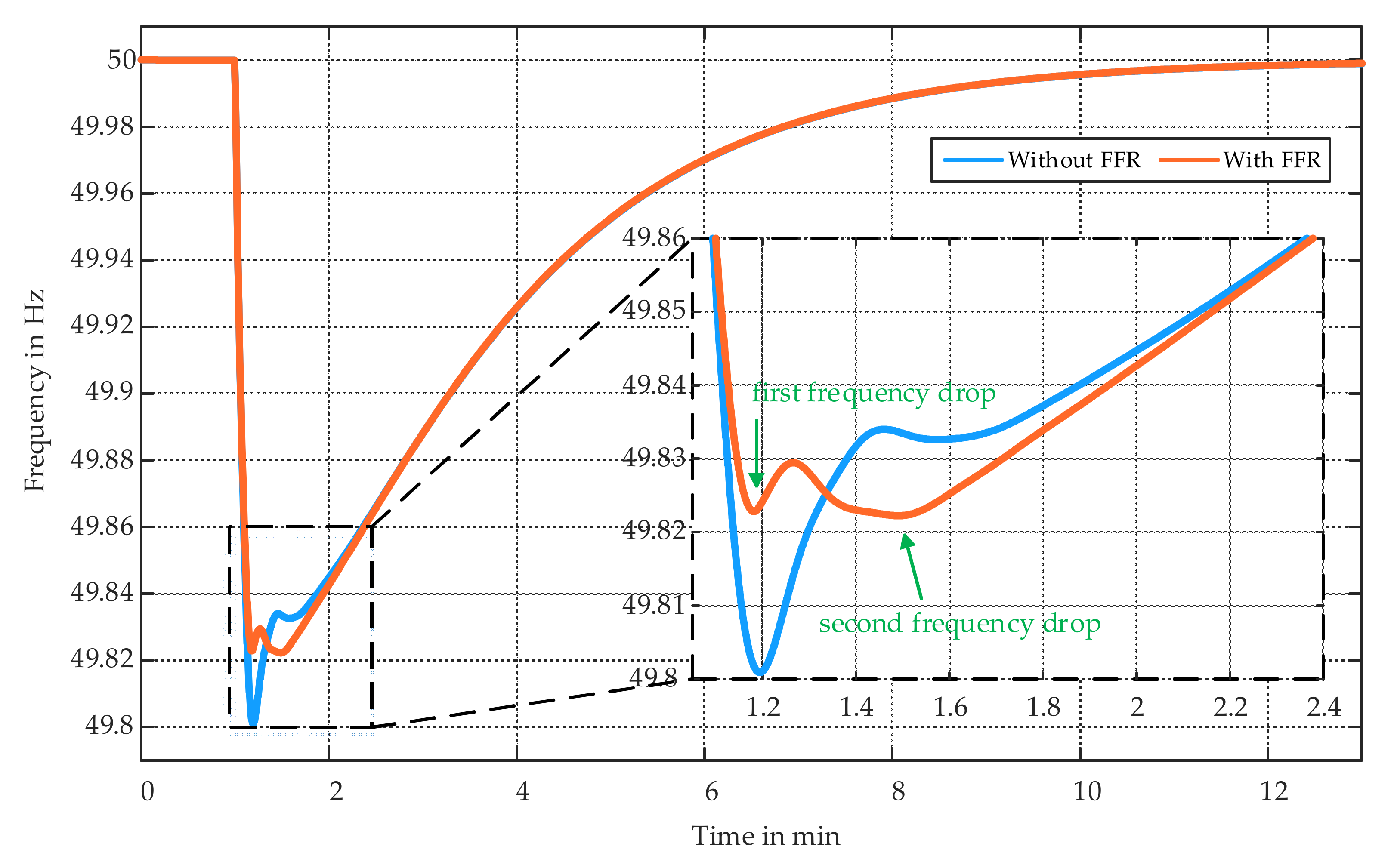
Figure 22 depicts the center of inertia frequencies in both scenarios with and without FFR controller activation. An improvement of 21.9 mHz in the FN is shown as a result of the FFR contribution of the WTs in the second scenario. An undesirable but unavoidable second frequency drop caused by the power reduction in the recovery phase is also observed, which is deeper the higher the maximum additional power achieved in the overproduction phase.
7. Discussion
As mentioned in
Section 6, the case studies are neither intended as a parameter analysis and tuning nor as a performance assessment of the FFR capability. Furthermore, a model validation in the context of comparative scenarios against, e.g., commercially available wind turbine models is outside of scope of this work. The authors consider such quantitative studies as a subject for future publications. This article is a modelling-oriented one, and the case study results serve primarily as examples to demonstrate the qualitative dynamic performance of the proposed WT model. The initialization results depicted in
Figure 16 are self-explaining and confirm very well-functioning initialization procedures. Step response simulation with deterministic wind speeds is a typical analysis approach to evaluate the general behavior of the WT at different operating points. The step response simulations lead to feasible results shown in
Figure 17 and
Figure 18, which are comparable with the results of the similar simulations represented in [
12]. The simulation scenarios to demonstrate the contribution of the WT models to improving the frequency performance of power systems provide plausible responses in the event of a frequency drop as depicted in
Figure 20 and
Figure 21, which are comparable with the simulation results represented in [
30,
36]. A striking point when comparing the results is that the slope of the overproduction phase (light blue curve in
Figure 20 and
Figure 21) can be modified by setting the minimum frequency limit
. The higher this frequency is set, the steeper the light blue curve becomes.
8. Conclusions
This article shows that a RMS DFIG-based wind turbine (WT) model and a RMS FSC-based WT model can be integrated into a combined overall model with little effort and the same set of parameters due to their high structural similarity. The presented model can be applied for classical network stability analyses. As an example, in order to illustrate the contribution of WT models to enhance the frequency behavior of power systems, it is extended with a droop-based fast frequency response (FFR) controller. In addition, well-functioning initialization procedures for both DFIG-based and FSC-based WT models are also introduced. The results of the executed case studies show plausible dynamic behavior of both WT models as well as feasible responses to a frequency drop in a 220 kV test system.
The modularity of the model offers the possibility of simple integration of other additional modules, which enable the WT models to respond appropriately to other stability issues and thus support power systems. Moreover, the model can be extended in future studies to include further converter control strategies (e.g., grid-supporting control concepts), which shall improve the stability of future power systems with a high penetration of power electronic-interfaced generating units.


