1. Introduction and Literature Review
Fighting against climate change is probably the largest challenge that humanity faces [
1]. If we are not able to reduce significantly, and in a short period of time, anthropogenic emissions of greenhouse gas (GHG), we risk facing catastrophic events that would compromise life as we know it in many parts of the world. This is the motivation behind international efforts such as the Paris Agreement [
2], in which all nations have agreed to make their best efforts at limiting the increase of temperatures below 1.5 °C above pre-industrial levels.
However, determining which is the right path towards that goal is not an easy task, due to several complicating issues:
- -
First, there is a lot of uncertainty both about the potential consequences of climate change, and also about how effective our actions against it will be;
- -
Second, our decisions face irreversibility in two ways. If we do nothing, life on Earth will suffer permanent damage. If we do too much, we may have wasted valuable resources;
- -
Third, given that climate change is a global externality, the actions of every region will influence the global outcome.
In many instances, the path and speed for the transformation of our economies is determined by estimating the social cost of carbon (SCC), the external cost of carbon emissions. The larger the SCC is, the larger the damages expected, and hence the larger the willingness to act against climate change. SCC is typically estimated using integrated assessment models (IAMs), complex models in which researchers try to represent how the climate or the economy work.
But again, due to the complexities mentioned earlier, developing good IAMs is not straightforward, which explains (at least in part) the academic discussions about the estimates of the social cost of carbon. Some scholars are focusing on the choice of parameters (e.g., the famous discussion about the higher costs of carbon obtained by the Stern review compared to previous estimates by Nordhaus, which was due to differences in the discount rates used [
3,
4,
5]), some on the capacity of IAMs (e.g., [
6,
7,
8]) to include all of the relevant issues (see e.g., Pindyck [
9], or Dietz et al. [
10]). Indeed, IAMs have become so complex, as more and more features are added to them, that they make it very difficult to understand intuitively their findings.
Therefore, some authors (being Pindyck [
11] probably the most vocal) advocate for the use of simpler approaches which are able to combine the major elements of the climate change problem but still can be understood intuitively.
For example, Golosov et al. [
12] proposed a dynamic stochastic general-equilibrium model for building a global economy-climate model. With this model, these authors try to find the optimal level of the tax on carbon that should be applied to minimize damages due to climate change. Gerlagh and Liski [
13] study the socially optimal pricing over time when climate change may cause stochastic catastrophes. The carbon price tends to increase with income. If past warming is not substantial enough for learning the true long-run social cost, the price should grow faster than the economy. It grows slower than the economy as soon as the warming generates information about events that could have arrived but have not done so. Their analysis concludes that the price increases roughly at the rate of the economy for the following 100 years. However, damages are a constant fraction of output and take place just once. Traeger [
14] tries to model the process by which temperatures will increase and uses a damage function based on a previously mentioned DICE model. Several simulations are implemented to find the optimal carbon tax with this approach too. Van der Ploeg and de Zeeuw [
15] model two effects of GHG accumulation on the economy, with a production that follows Golosov et al., and also have a single tipping point, which causes a gradually increasing proportional drop in output. Finally, Hassler and Krusell [
16] model the multiregional aspect with a stochastic general equilibrium which allows them to analyze the spillovers of policies. However, they do not allow for a technological solution to the problem.
Besley and Dixit [
17] try to solve many of the shortcomings of the previous literature. They develop a simple, tractable model, which can be understood intuitively, and which represents the most important features of the climate change problem: (i) that neither the occurrence nor the costs of a catastrophic event in any one year are precisely predictable; (ii) that the probability of a catastrophe occurring in any one year increases with GHG levels; (iii) that GHGs are a worldwide public bad; emissions from any one country or region increase the risks for all; (iv) that there is a two-sided irreversibility of policies; and finally (v), that technology may solve the problem by removing carbon from the atmosphere (or some other form of geoengineering).
Their model is a dynamic one, in which there is a certain probability of a catastrophic event (which is an increasing function of GHG concentrations in the atmosphere). The catastrophe is modeled as a Poisson process. GHG concentrations are a function of emissions, accounting for dissipation or absorption into water and land masses. Emissions in turn are a constant function of GDP. The authors also model another independent Poisson process which represents a technological solution to climate change and would reduce the damages of climate change (but not emissions, so it could be considered a form of adaptation or geoengineering). With this model, the authors derive expressions for compensating and equivalent variations to measure willingness to pay (as a fraction of GDP).
Under several assumptions further detailed in their paper, Besley and Dixit find that individual countries would be willing to pay a cost of 3.3% of GDP each year to bring about reductions equivalent to those agreed under the Kyoto Protocol (which are much smaller than those pledged in the Paris Agreement). When multiple regions are considered, the willingness to pay is similar if all countries keep their pledges. The amount decreases if other regions defect from the agreement, if future growth is lower, or if damages in that region are smaller than average. In most cases, the willingness to pay is above 1% of GDP. The model is therefore able to inform us about the order of magnitude of the sacrifices that societies would be willing to make to reduce the risk of climate change, and how they change depending on the actions of other regions. However, the model has some limitations that make it not completely realistic.
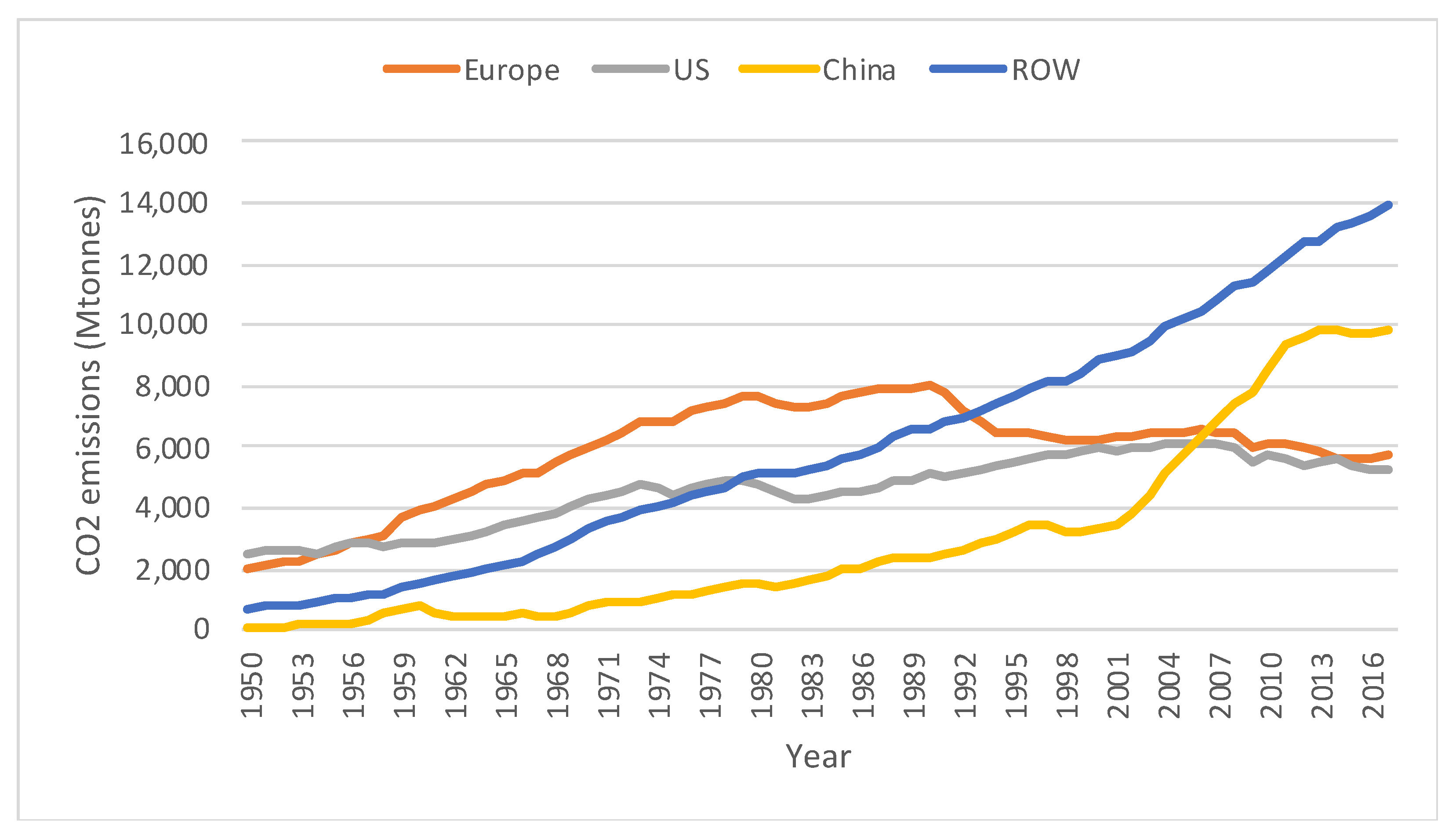
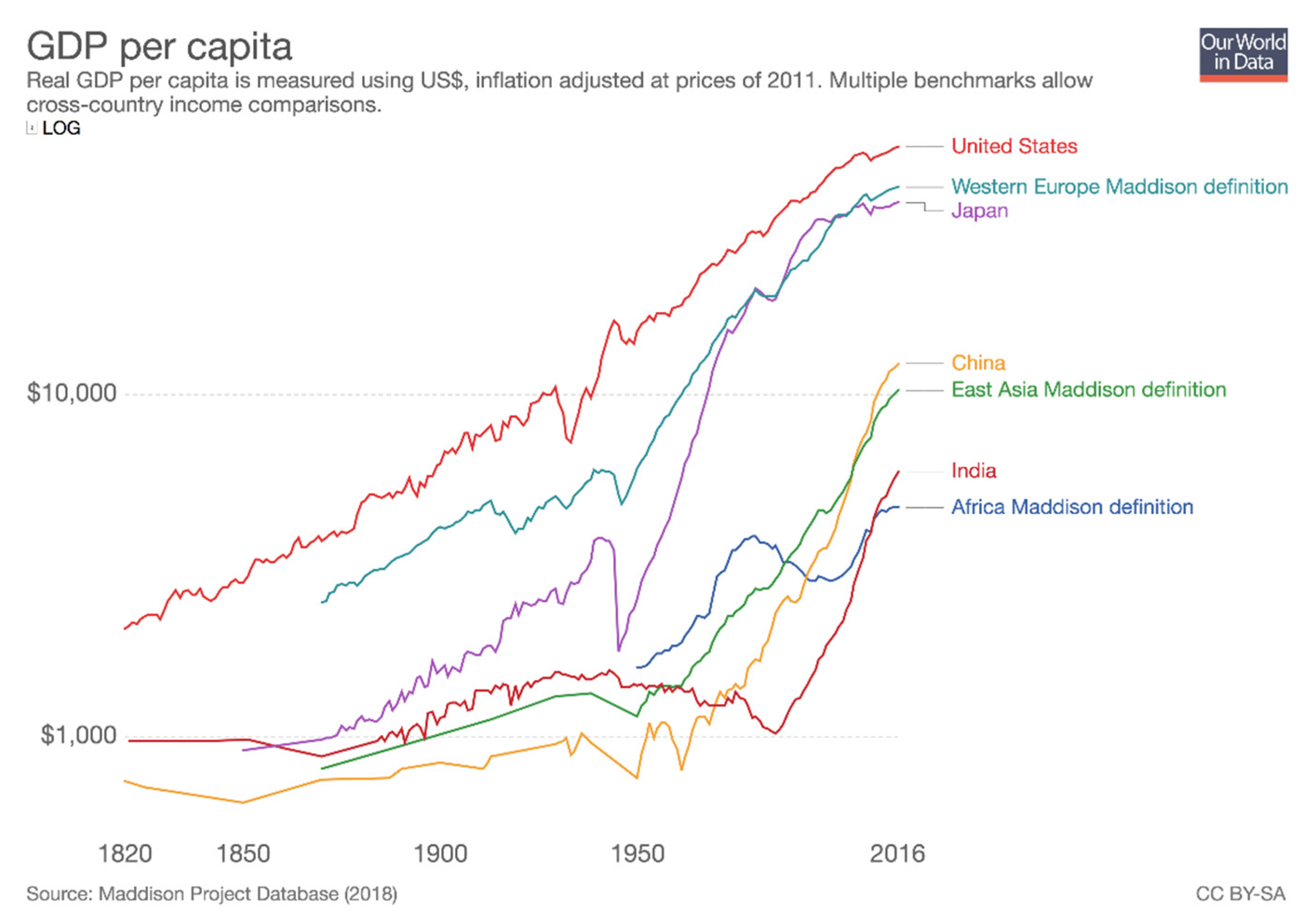
First, the relationship between emission flows and GDP is assumed to be constant. But this is clearly not true, as the relationship between those variables has changed during the last decades, thanks to the increased contribution of energy efficiency and low-carbon energy sources, as well as due to the tertiarization of most economies.
Figure 1 and
Figure 2 illustrate the evolution of emission flows and GDP for different regions in the world. It can be observed how the relationship between emission flows and GDP growth has been modified in several regions since the last decades of the twentieth century until now.
The second problem is that the model only considers technological advance as the possible appearance of a technological ‘miracle’ that would not reduce emissions but rather eliminate their negative consequences (adaptation or geoengineering). This technological ‘miracle’ is modelled as a Poisson process. However, although adaptation is probably a must, given the advance of climate change, geoengineering technologies remain controversial given their many downsides (see e.g., [
19]).
Given the recent evolution of renewable technologies or carbon capture and use, it would make much more sense to model a technology that actually reduces GHG emissions, and hence decouples economic growth and GHG emissions. A way of representing the probability of this group of technologies is to model it as a Poisson process. Then, the relationship between emission flows and GDP can also be made variable instead of fixed. This, in turn, may also change the willingness to pay, and its relationship to the other parameters.
The goal of this paper, then, is to improve the already comprehensive and intuitive Besley and Dixit’s model by including a backstop technology (e.g., a competitive renewable energy source such as solar PV, either alone or combined with green hydrogen) that allows one to decouple economic growth and GHG emission. This is in fact the globally preferred option for reducing the impacts of climate change, as can be currently seen in energy transitions across the world. By doing this, we are able to provide a much more realistic model to understand intuitively the factors affecting the willingness to pay for avoiding climate change, without the need to use a more complex IAM, and hence to understand better the level of effort required to fight against climate change, something absolutely pertinent currently as all countries are revising their nationally determined contributions to the Paris Agreement.
In
Section 2 we describe the improvements in the model, and in
Section 3 we present some of the results obtained, which are then discussed in
Section 4.
Section 5 offers some conclusions.
2. Materials and Methods
We start from the basic formulation provided by Besley and Dixit. Their model starts by computing the expected net present value,
V(
xt) of all relevant economic and monetary equivalent non-economic benefits and costs depending on the GHG concentration log-level,
xt, which in turn depend on the (unpredictable) possibility of occurrence of the climate catastrophe and of the technological solution. These possibilities also depend on the GHG concentration level.
On the right-hand side, each line corresponds to an outcome of the two Poisson processes. The first process is the catastrophe, which has an arrival rate λ(xt); the second is the technological solution with an arrival rate μ(xt). The arrival rate of the catastrophe is modeled as a logistic function: , where γ and J are parameters for the arrival rate of the catastrophe.
In the first line, both the catastrophe and the technological solution occur; this incurs the cost and generates the present value of the GDP stream calculated as . In the second line, the catastrophe occurs but the technological solution does not arrive. This incurs cost , has the immediate GDP flow , and yields the continuation value starting next year so discounted back by the factor 1/(1 + r), where r is the discount rate. In the third line there is no catastrophe in period t and the technological solution arrives, so we simply get the present value of the GDP stream. In the fourth line neither the catastrophe nor the technological solution takes place, so we have the immediate GDP flow and the continuation value.
xt, the GHG concentration level, is a function of the permanent stock
Pt and of the dissipating stock
St.
Pt is a fraction
ε of the emission flow in period
t, zt,
and
St grows as
where
δ is the dissipation rate.
Now, as explained in the introduction, we improve the original model by introducing the possibility of developing a backstop technology (e.g., a renewable energy technology) that will reduce GHG emissions. Let μ′ represent the probability of that technology to appear. It can be modelled as a Poisson process whose arrival rate will be . We assume that depends on GDP: the higher the GDP the higher the amount of money destinated to R&D, and therefore the higher the probability to develop this technology. The new formulation is presented below, where all parameters and variables are the same as in the original model except for .
The explanation of what this expression represents is the same one of the original model with one exception. It considers an additional Poisson process that considers the possibility of a cheap technology with the ability to reduce emissions to appear. If this is the case, future emissions will not increase, and therefore is replaced by for the period t + 1. The rest of the logic is similar to the one explained earlier. Elaborating on the expression, we obtain the following, with g being GDP growth.
Then, the expected net present value of the economy at year 0 is:
where
Being
D(
t) the risk-corrected discount factor. The expression above can be derived to obtain a new expression for substituting in the original model. Iterating the equation for
DT+1 starting at
and going up to
T we have:
As
for all t, if
we have:
In order to carry out a numerical analysis of the model, some assumptions need to be made as in the original model: The first one consists in considering that compensating variations and equivalent variations are exactly the same. In addition, the cost associated with natural disasters if they occur is assumed to grow at a fixed rate g (that is, the same rate at which the GDP keeps on growing too).
The probability of a technological solution to appear is assumed to be constant for all years. It will be represented by μ. In addition, it will be assumed that the approximation of considering that μ′ is constant for all future years is reasonable to solve the model.
With these assumptions, the expected net present value of the economy can be calculated by simplifying the former expressions as follows.
where
Λ is the expected discount cost of catastrophes. This expression is more complex than the simplified one obtained in the original model. However, it constitutes a more realistic approach.
Finally, the last modification that will be introduced in this model compared to the original one is to consider αt, the relationship between GDP and GHG emissions, as a variable instead of a constant. When the probability of a cheap technology with the ability of reducing emissions exceeds a value of 99%, αt will be zero for all future years. For the previous years it will be equal to α.
For the sake of brevity, we do not include the rest of the equations of the model. Interested readers may consult them in Besley and Dixit [
17].
3. Results
In this section we solve the model for the same set of parameters as in Besley and Dixit, in order to compare the outcomes and assess the impact of introducing a backstop technology into the model. The only additional parameter is μ′, the arrival rate for the backstop technology, which in this case has been assumed to have a larger probability than the arrival rate for the geoengineering technology.
3.1. Input Parameters
The default case in this improved model corresponds to the following values for the input parameters, shown in
Table 1:
The first aspect that should be pointed out is that the growth rate of emission flows varies with time instead of being fixed. The reason for this is that we are considering now the effects of 2% of annual probability for a cheap technology with the ability of reducing significantly emission flows in all regions, and therefore emissions are reduced in future years under this circumstance. This is a more realistic approach than considering just the possibility of a technological ‘miracle’ to happen. If this is not taken into account, the impact of not committing with the Paris Agreement triggers higher emission flows in the future, and therefore the economic impact is much higher too.
The default values for μ′ will be 0.02 for all regions, given that the probability of this technology to appear seems larger than the probability of developing a valid geoengineering technology. These values will be further modified for analyzing different scenarios. With this numerical approach, the probability of this type of technology to appear within the next 35 years is approximately 50%.
3.2. Results
Table 2 presents the results of the willingness to pay against climate change for different choices of the parameter set.
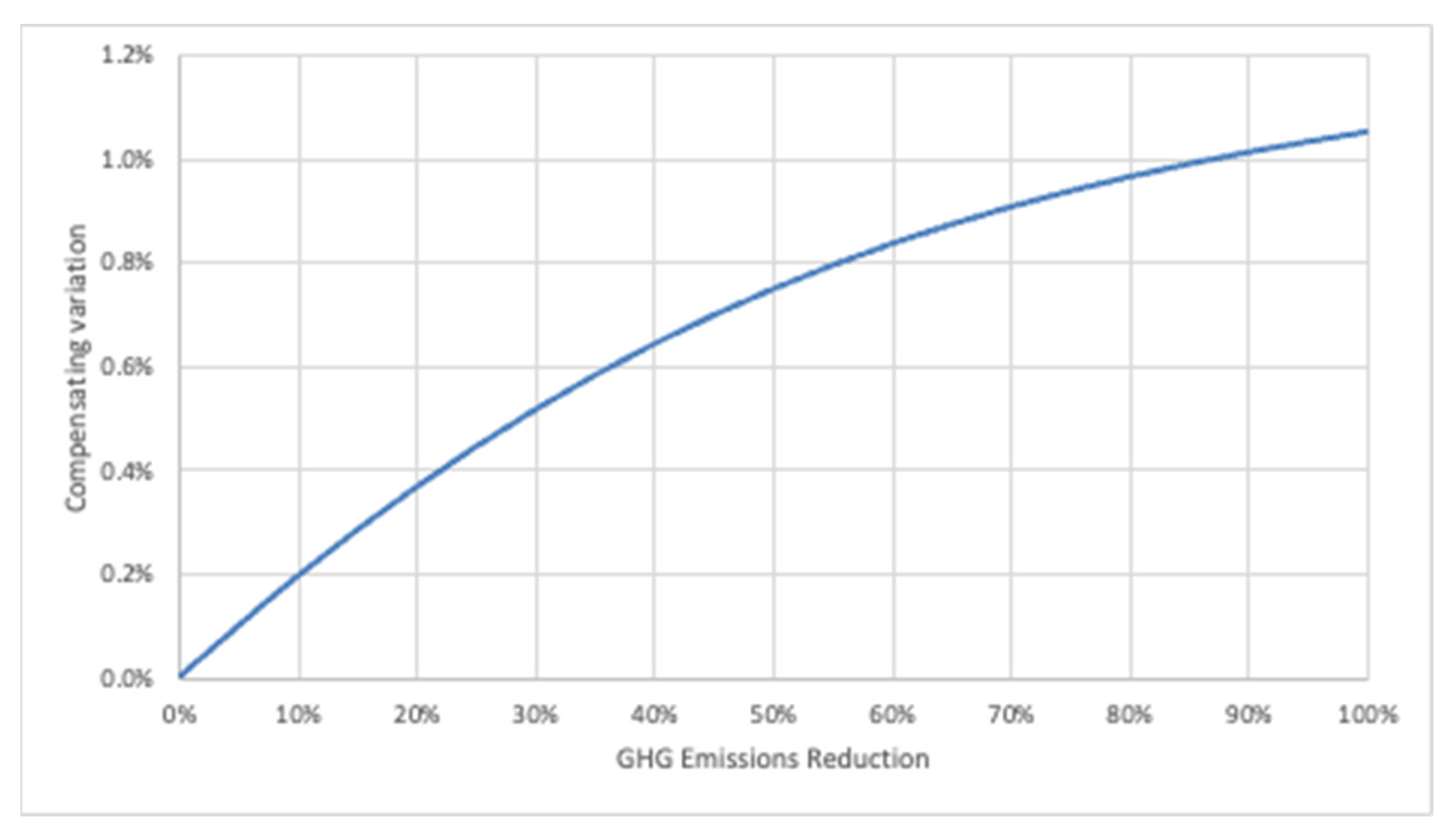
We have also tested the sensitivity of the willingness to pay to different degrees of ambition in the reduction of emissions. The results are shown in
Figure 3.
4. Discussion
Under the baseline parameters, and for the 30% reduction of emissions assumed by Besley and Dixit, our results show that each region would be willing to pay 0.52% of their annual GDP to avoid the possibility of a climate change catastrophe. This is much lower than the 3.3% obtained by the original model, and makes sense since now we have introduced a more flexible and more probable option to fix the problem. Indeed, when we reduce the probability of finding the low-carbon alternative to 0.01, the willingness to pay increases to 1.24%; we are willing to sacrifice more of our GDP to ensure that we will not incur in a catastrophe.
On the other hand, a 50% improvement in the chance of finding the low-carbon technology to 0.03 results in a reduction of WTP to 0.24%. That means that we could spend the difference (0.28% of GDP) in investing to improve this chance.
If instead we assess how much we would be willing to invest in the “geoengineering” technology, the benefit is lower, and hence the difference in WTP is now 0.26% of GDP. This shows the advantages of investing in mitigation technologies, which result in lower accumulation of GHG in the atmosphere and hence in lower risks and eventually lower geoengineering costs.
Of course, this estimate would change if we introduced a different value for K0/y0. This factor represents the relationship between the cost caused by natural disasters and annual GDP. Besley and Dixit used as a reference the damages caused by hurricane Katrina, but this does not necessarily indicate the magnitude of the damages expected from climate change. If we increase the factor to 3, then the willingness to pay increases to 0.78%, still below 1% of GDP (and hence an amount that should be easy to command if there is the political will). However, if we reduce it to 1, then WTP is reduced to 0.26%.
Thanks to formulating the problem as a multi-region model, we are also able to account for differences in the willingness to pay between regions when actions against climate change differ, when the damages are not homogeneous, or when growth rates are different.
For example, if China did not engage in substantial action, then the willingness to pay of the rest of the regions would fall to 0.36%. This fall is more significant than if it is the US the one who opts out (then WTP would be 0.44%), due to the larger emissions share of China. If only the three larger economies engage in significant GHG emission reductions, but the rest of the world does not follow suit, then willingness to pay would be reduced to 0.31%.
Another interesting question is what would happen if only Europe goes for significant GHG emissions reductions (as stated in their Green New Deal). In this case, the willingness to pay of that region would be reduced to 0.11%, showing how unilateral action, without the participation of other regions, is much less valuable. This of course reinforces the case for a concerted action, and in the case of Europe, for its push for climate diplomacy as a way to engage other regions in similar emissions reductions.
Willingness to pay is also determined by the severity of the damages, as shown earlier. But this will be clearly different among regions. While more developed regions may have more resources to adapt to climate change, other regions will clearly suffer larger damages (see e.g., [
20]). If we assume that K0/y0 increases to 4, but only for the ROW region, then we find that the WTP in that region would increase to 1.03%, while the rest stays at 0.52%. Of course, the question here is how these typically poorer countries will be able to finance that expenditure, and the impact that this may have on global inequality.
Different rates of growth also imply different WTP estimates: if growth is reduced to 1% in the US and Europe, and maintained in China and ROW, that means that the willingness to pay of the lower-growth regions is also reduced to 0.26%, while the rest stays at 0.52%. In this case, however, the higher WTP can be financed with the larger growth rate.
Finally, a very relevant simulation is one in which we increase the reduction in GHG emissions required. Besley and Dixit assumed a 30% reduction, consistent with the Kyoto Protocol. However, the Paris Agreement requires a much larger reduction if we are to comply with the 1.5–2 °C threshold. We have therefore calculated the sensitivity of the willingness to pay for different levels of emissions reductions, which is shown in the following figure.
As may be observed in
Figure 3, under the baseline scenario, the willingness to pay increases with the stringency of emissions reductions until it reaches 1.1% of GDP. This may be compared with the results from Besley and Dixit, which obtained a maximum figure of 7% GDP. Again, this shows the benefit of including an emissions reduction technology in the model, which provides additional flexibility to containing the severity of climate change.
It should also be noted that the increase in WTP is reduced when emissions reductions are larger. This is a natural result, given that when emissions are lower, the probability of a climate change catastrophe is also lower, and hence the willingness to pay for avoiding it is lower.
5. Conclusions
In this exercise we have modified an existing simple model to estimate the willingness to pay of different regions in order to avoid catastrophic climate change. The changes involved have been the introduction of the possibility of developing competitive low-carbon technologies such as renewables, or carbon capture and use, which are in fact the globally preferred options for reducing the impacts of climate change, as can be currently observed in energy and climate transitions across the world (and also by extending the simulation to include GHG emission reductions compatible with the Paris Agreement). By doing this, we contribute to a better and more realistic understanding of the level of effort required to fight against climate change, and of the factors that influence that effort. This is an absolutely central topic in the preparation of the Nationally Determined Contributions that all countries are preparing and revising under the Paris Agreement.
Our major conclusion is that, first, the willingness to pay to avoid catastrophic climate change is significant, but limited, varying from 0.25% to 1% of annual GDP. This is in our opinion a perfectly manageable sum, in particular if there is coordination among regions so that this cost is shared. Our results also show the benefit of including into the model the possibility of developing a competitive, zero-carbon technology, that would allow us to eliminate emissions. That technology has clear benefits over geoengineering alternatives, since reducing emissions results in lower carbon stocks in the atmosphere, and therefore in lower risks for the future.
A second interesting insight is that unilateral action results in a reduction of willingness to pay (since benefits are enjoyed by other regions). This reduction is larger the smaller the contribution of that region to global emissions. For example, if only Europe takes significant action against climate change, its willingness to pay would be very small, 0.11% of GDP. This clearly justifies the need to promote concerted action, as exemplified by the Paris Agreement. This concerted action should also take into account differences in the damages suffered in the various regions, as well as potentially diverging growth rates: increased growth rates result in higher WTP figures (since there is more at stake). Larger damages also imply increases in the willingness to pay; however, if these larger damages take place in developing regions, the question is how to finance the required expenditures, given the impact that this may have on the fight against climate change but also on global inequality.
As in the original paper, several limitations remain. The most important in our view is the assumption that growth is not affected permanently, but only temporarily, by climate change. However, we still think that the simple model proposed is able to provide important insights about the willingness to pay for avoiding catastrophic climate change, into the interplay between different relevant parameters, and also to show the interconnection between different regional attitudes towards climate change. As we said before, these are essential elements in the current international negotiations within the Paris Agreement now and in the years to come.


