Flight Stability of Rigid Wing Airborne Wind Energy Systems

Abstract

The flight mechanics of rigid wing Airborne Wind Energy Systems (AWESs) is fundamentally different from the one of conventional aircrafts. The presence of the tether largely impacts the system dynamics, making the flying craft to experience forces which can be an order of magnitude larger than those experienced by conventional aircrafts. Moreover, an AWES needs to deal with a sustained yet unpredictable wind, and the ensuing requirements for flight maneuvers in order to achieve prescribed control and power production goals. A way to maximize energy capture while facing disturbances without requiring an excessive contribution from active control is that of suitably designing the AWES craft to feature good flight dynamics characteristics. In this study, a baseline circular flight path is considered, and a steady state condition is defined by modeling all fluctuating dynamic terms over the flight loop as disturbances. In-flight stability is studied by linearizing the equations of motion on this baseline trajectory. In populating a linearized dynamic model, analytical derivatives of external forces are computed by applying well-known aerodynamic theories, allowing for a fast formulation of the linearized problem and for a quantitative understanding of how design parameters influence stability. A complete eigenanalysis of an example tethered system is carried out, showing that a stable-by-design AWES can be obtained and how. With the help of the example, it is shown how conventional aircraft eigenmodes are modified for an AWES and new eigenmodes, typical of AWESs, are introduced and explained. The modeling approach presented in the paper sets the basis for a holistic design of AWES that will follow this work.

1. Introduction

Airborne Wind Energy (AWE) is the field of wind energy which aims at harvesting power from the wind through airborne systems. Airborne Wind Energy Systems (AWESs) can access wind resources at higher altitudes and they can obtain the same power output of conventional wind turbines with a drastic reduction of mass, which could lead to a cost decrease [1,2]. Many concepts are being developed and they are classified according to how the aerodynamic force, needed for the power production, is generated. A classification of the currently pursued AWE concepts, their flight operations and developers is given in [3]. The present paper is focusing on the development of AWESs which produce aerodynamic force by flying crosswind. Crosswind AWESs can generate power in two ways [3]: with on-board wind turbines (Fly-Gen AWESs) or with a generator placed at the ground station (Ground-Gen AWESs), which can be fixed or moving [3]. Fly-Gen AWESs produce power on board and transmit it to the ground station through electric wires embedded in the tether [4,5]. Ground-Gen AWESs with fixed ground station produce power cyclically. In the power generation phase, they produce power by pulling and unwinding the tether, which is connected to a generator. In the recovery phase, they fly back, spending some power, while the tether is wound back. Ground-Gen AWESs are being developed with soft kites [6,7] or rigid wing aircrafts [8,9,10].

To become a viable alternative to conventional wind turbines, AWESs flying crosswind need to display a sufficient reliability, thus allowing operations over long time frames. Therefore, design choices should keep robustness to external disturbances and failures as a premium goal. This in turn can be achieved through an increased knowledge of the dynamics of the flying craft, as a means to quantify how some characteristics of the AWES impact its performance, so as to allow suitably sizing the machine to meet all expectations.

The flight mechanics problem of AWESs is fundamentally different from the one of conventional aircraft for mainly three reasons: the presence of the wind, needed for the power generation (the average wind speed does not influence conventional aircraft flight stability analyses, as the inertial coordinate system can be considered to move with the average wind speed, but this is not the case for AWES), the presence of the tether, which transfers all forces acting on the airborne unit to the ground, and the need for maneuvers to keep the aircraft in the correct trajectory and attitude. It is therefore clear that conventional design techniques assuming straight and level flight can hardly be used for AWESs.

Makani Power [4], before the shutdown, started investigating the possibility of designing the flight path and aerodynamic characteristics of the AWES to achieve passive stability [11,12]. Stable AWESs would maintain the flight path with the least amount of control activity. Previous works [13,14,15] analyze the flight stability of kites not undertaking the crosswind motion for power generation. In this work, the kite crosswind motion needed for power generation is included in the analysis.

To achieve stability, the flight path should be properly chosen: a circular path makes the problem nearly axial-symmetric, and there exists one turning radius which ensures maximum tether force and potentially maximum power production [16]. As this turning radius maximizes the tether force, a stable-by-design AWES, if perturbed from this path, would tent to return to the operational point which maximizes tether force. This flight path is then selected for the present investigation.

The AWES aerodynamic design should help, as much as possible, the control system to achieve robust operations. An analytical modelling approach to study flight stability is presented in this text. The six d.o.f. equations of motion are linearized about a fictitious steady-state motion of the AWES in the circular path. No real steady-state can be achieved during power generation because of the continuous maneuvers of AWESs. Indeed, gravitational forces and aerodynamic forces related to the mean elevation angle act periodically on the kite. The fictitious steady-state motion, also called trim in this paper, is then computed by considering all the fluctuating terms as disturbances. The peculiarity of the selected flight path is that, if the fictitious steady-state is considered, centrifugal forces, induced by the constant turning maneuver, are balanced by the radial component of the force on the tether. In this way, lift is not used for the turn maneuver. The derivatives of external forces and moments are finally taken about the fictitious steady-state, to formulate the linearized problem.

Finally, the stability of the system can be studied by looking at the eigenvalues of the linearized system. The procedure to study stability is summarized in Figure 1.

The linearized model allows for a simplified investigation of the influence of main wing geometry (position, area, aspect ratio, sweep, dihedral), main wing aerodynamics, control surfaces aerodynamics and geometry (area, aspect ratio, position), tether attachment position, tether mechanical and aerodynamic properties and mass properties of the AWES on flight stability. Also, since it does not primarily impact the dynamics of the flying craft, in this paper the power generation mechanism is not modeled. In this way, the model presented here can be used, with small modifications, to model both Ground-Gen and Fly-Gen AWESs.

As previously stated, the so-obtained model of the plant allows a good physical understanding of the effect of design choices on performance, and especially on stability. This in turn enables the formulations of design guidelines for the geometry and aerodynamics of rigid wing AWESs. Furthermore, the quality and characteristics of the model introduced in this paper bends itself to an adoption inside iterative optimal design tools, as well as for control design and tuning tasks.

An AWES designed to be stable, with the approach proposed in this work, has no guarantees to converge to the prescribed trajectory without control inputs. The formulation proposed here is meant to study the system dynamics of the AWES set to a state representative of its flight during the power generation loop. Therefore, the term stability in this paper refers to the ability of the system of returning to the fictitious steady-state if perturbed from it. As the fictitious steady-state is representative of the flight during the power generation loop, flight dynamic performances and control efforts over the loop are expected to benefit from a stable design.

The paper is organized as follows. Section 2 presents the non-dimensional linearized equation of motion derived for a generic AWES and Section 3 deals with the derivation of the external forces acting on the AWES. These two sections represent the mathematical basis for this paper and for subsequent work on the holistic AWES design and are therefore intended to be very comprehensive and detailed. Section 4 deals with the numerical implementation of the above mathematical model in MATLAB^®, while Section 5 presents a preliminary validation of this tool. Finally, Section 6 reports the results for different sets of configurations of increasing complexity and Section 7 closes the manuscript summarizing the main findings of this research.

2. Linearized Equations of Motion

2.1. Coordinate Systems

Three coordinate systems are defined to derive the equations of motion. The ground coordinate system ${\mathcal{F}}_G$ (Figure 2) is centered at the ground station and it is inertial. Its origin is denoted as G. $Z_G$ points upwind and $X_G$ toward the ground. ${\mathcal{F}}_G$ can also be interpreted as the wind reference frame. As ${\mathcal{F}}_G$ is treated as an inertial frame, the inertial force components caused by the rotation of the wind vector are neglected.

A second coordinate system ${\mathcal{F}}_R$ (Rotating) is defined such that it moves on a circumference of constant radius $R_0$, rotating around its $Z_R$ axis: $X_R$ points along the tangential direction and $Y_R$ outward. $X_R$ and $Y_R$ define the rotor plane (Figure 2). The origin of ${\mathcal{F}}_R$ is named R and lies on the plane connecting the ground station, the circumference center and the tether attachment point on the kite. With this definition, ${\mathcal{F}}_R$ does not have a constant rotational speed.

The rotation matrix ${\mathbf{R}}_{G\to R}$, which describes a coordinate transformation from ${\mathcal{F}}_G$ to ${\mathcal{F}}_R$, is defined by two sequential planar rotations, associated with the mean elevation angle $\beta$ and the angular position $\Psi$ of ${\mathcal{F}}_R$ along the circumferential trajectory of the craft (see Appendix A for rotational matrix notation)

$$\begin{array}{cc}\hfill {\mathbf{R}}_{GR}^G\left(\Psi ,\beta \right)& ={\mathbf{R}}_{G^{\prime }R}^G\left(\Psi \right){\mathbf{R}}_{G{G}^{\prime }}^G\left(\beta \right)={\mathbf{R}}_{y,G{G}^{\prime }}^G\left(\beta \right){\mathbf{R}}_{z,G^{\prime }R}^{G^{\prime }}\left(\Psi \right).\hfill \end{array}$$

(1)

The stability coordinate system ${\mathcal{F}}_S$ (Figure 3) is centered at the tether attachment point and is moving and rotating with the kite. Its origin is denoted as S. Equations of motion are written in ${\mathcal{F}}_S$, which makes the formulation of the external forces compact. As ${\mathcal{F}}_S$ is defined from the aircraft trajectory, and not from a reference frame attached to the kite, inertial and geometrical properties of the system need to be expressed in ${\mathcal{F}}_S$ for each operational point (i.e., wind speed). This procedure is detailed in Section 4. The rotation matrix which describes a coordinate transformation from ${\mathcal{F}}_R$ to ${\mathcal{F}}_S$ is defined with three sequential planar rotations, around the third, second (rotated) and first (rotated) axes of the frame respectively

$$\begin{array}{cc}\hfill {\mathbf{R}}_{RS}^R\left(\varphi ,\theta ,\psi \right)& ={\mathbf{R}}_{R^{\prime \prime }S}^R\left(\varphi \right){\mathbf{R}}_{R^{\prime }{R}^{\prime \prime }}^R\left(\theta \right){\mathbf{R}}_{R{R}^{\prime }}^R\left(\psi \right)={\mathbf{R}}_{z,R{R}^{\prime }}^R\left(\psi \right){\mathbf{R}}_{y,R^{\prime }{R}^{\prime \prime }}^{R^{\prime }}\left(\theta \right){\mathbf{R}}_{x,R^{\prime \prime }S}^{R^{\prime \prime }}\left(\varphi \right).\hfill \end{array}$$

(2)

In steady-state, ${\mathcal{F}}_S$ and ${\mathcal{F}}_R$ coincide. Thus, this definition of coordinate systems is particularly useful when studying perturbations about the steady-state, which is the case in the formulation adopted in this paper.

As the final aim of this work is to linearize the system about its steady-state, $\left(\varphi ,\theta ,\psi \right)$ are assumed to be small and ${\mathbf{R}}_{RS}^R$ is linearized, so that

$$\begin{array}{cc}\hfill {\mathbf{R}}_{RS}\left(\varphi ,\theta ,\psi \right)& \approx \left[\begin{array}{ccc}1& -\psi & \theta \\ \psi & 1& -\varphi \\ -\theta & \varphi & 1\end{array}\right]=\mathbf{1}+{\left[\begin{array}{c}\varphi \\ \theta \\ \psi \end{array}\right]}^{\times }=\mathbf{1}+{\mathbf{Eu}}^{\times },\hfill \end{array}$$

(3)

where $\mathbf{1}$ is the 3 by 3 identity matrix and the symbol ${(·)}^{\times }$ applied to a vector represents its corresponding skew-symmetric tensor form. With these assumptions, ${\mathbf{R}}_{SR}={\mathbf{R}}_{RS}^T=\mathbf{1}-{\mathbf{Eu}}^{\times }$.

2.2. Position

To formulate the equations of motion in ${\mathcal{F}}_S$ and evaluate the tether elastic force, the position of the ground station with respect to ${\mathcal{F}}_S$, expressed in ${\mathcal{F}}_S$ (${\mathbf{X}}_{S\to G}^S$), is to be found. It can be expressed as the summation of ${\mathbf{X}}_{S\to R}^S$ and ${\mathbf{X}}_{R\to G}^S$:

$$\begin{array}{cc}\hfill {\mathbf{X}}_{S\to G}^S& ={\mathbf{X}}_{SR}^S+{\mathbf{X}}_{RG}^S={\mathbf{R}}_{SR}\left({\mathbf{X}}_{SR}^R+{\mathbf{X}}_{RG}^R\right),\hfill \end{array}$$

(4)

where

$${\mathbf{X}}_{RG}^R=\left[\begin{array}{c}0\\ -R_0\\ Z_0\end{array}\right],{\mathbf{X}}_{SR}^R=-\left[\begin{array}{c}{x}_{rs}\\ y_{rs}\\ z_{rs}\end{array}\right],$$

(5)

with $R_0$ the circular path radius, $Z_0$ the distance of the ${\mathcal{F}}_G$ from the rotor plane AA (see Figure 2) and ${\mathbf{X}}_{RS}^R={\left[x_{rs},y_{rs},z_{rs}\right]}^T$ (see Figure 3).

2.3. Angular Velocity

The angular velocity of ${\mathcal{F}}_S$ with respect to ${\mathcal{F}}_G$, expressed in ${\mathcal{F}}_S$ takes the form

$$\begin{array}{cc}\hfill \mathit{\omega }\equiv {[p,q,r]}^T={\mathit{\omega }}_{GS}^S& \approx {\mathbf{R}}_{SR}^R{\mathit{\omega }}_{GR}^R+\dot{\mathbf{Eu}}=(\mathbf{1}-{\mathbf{Eu}}^{\times }){\mathit{\omega }}_{GR}^R+\dot{\mathbf{Eu}}.\hfill \end{array}$$

(6)

2.4. Relative Wind Speed

The wind velocity is along the $Z_G$ axis and has a negative direction. A constant and uniform wind field, parallel to the ground, is considered. Its definition by components in the stability coordinate system can be written as

$$\begin{array}{cc}\hfill {\mathbf{V}}_{w,\Psi }^S& ={\mathbf{R}}_{SG}^G\left[\begin{array}{c}0\\ 0\\ -V_w\end{array}\right]=-V_w\left(\mathbf{1}-{\mathbf{Eu}}^{\times }\right)\left[\begin{array}{ccc}{c}_{\Psi }& s_{\Psi }& 0\\ -s_{\Psi }& c_{\Psi }& 0\\ 0& 0& 1\end{array}\right]\left[\begin{array}{c}-s_{\beta }\\ 0\\ c_{\beta }\end{array}\right].\hfill \end{array}$$

(7)

In the formulation of dynamic equilibrium, the fluctuating terms, functions of $\Psi$, are considered as disturbances. Therefore, ${\mathbf{V}}_{w,\Psi }^S$ can be decomposed in a non-fluctuating and a fluctuating term

$$\begin{array}{ccc}\hfill {\mathbf{V}}_w^S& =-V_w{c}_{\beta }\left[\begin{array}{c}-\theta \\ \varphi \\ 1\end{array}\right],{\mathbf{V}}_{w,fl}^S\hfill & \hfill =-V_w{s}_{\beta }\left(\mathbf{1}-{\mathbf{Eu}}^{\times }\right)\left[\begin{array}{c}-c_{\Psi }\\ s_{\Psi }\\ 0\end{array}\right].\end{array}$$

(8)

The fluctuating term ${\mathbf{V}}_{w,fl}^S$ needs to be considered when studying the system in the time domain. Furthermore, for systems with no elevation angle, the fluctuating terms are null. This case is representative of a setup where the ground station is set on top of a tower or other elevated anchor points. The contribution of the fluctuating terms is along the $X_S$ and $Y_S$ axes. On the $X_S$ axis, the relative wind is dominated by the kite motion, while on $Y_S$ axis the kite experiences the fluctuating terms as side-slip velocities.

By considering a generic position in ${\mathcal{F}}_S$, namely ${\mathbf{X}}^S={[x,y,z]}^T$, the undisturbed relative wind speed ${\mathbf{V}}_r^S$ in ${\mathcal{F}}_S$ is defined as the the subtraction of the kite motion from the wind velocity, yielding

$$\begin{array}{cc}\hfill & {\mathbf{V}}_r^S\equiv -\left[\begin{array}{c}\mathcal{U}\\ \mathcal{V}\\ \mathcal{W}\end{array}\right]={\mathbf{V}}_w^S-\mathbf{V}-{\omega }^{\times }{\mathbf{X}}^S=-V_w{c}_{\beta }\left[\begin{array}{c}-\theta \\ \varphi \\ 1\end{array}\right]-\left[\begin{array}{c}u+zq-yr\\ v+xr-zp\\ w+yp-xq\end{array}\right],\hfill \end{array}$$

(9)

where $\mathbf{V}\equiv {[u,v,w]}^T={\mathbf{V}}_{GS}^S$ is the velocity of ${\mathcal{F}}_S$ with respect to ${\mathcal{F}}_G$, expressed in ${\mathcal{F}}_S$. The trim state (fictitious steady-state) is indicated in this paper with the subscript 0, therefore yielding for the baseline condition

$$\begin{array}{cc}\hfill & {\mathbf{V}}_{r0}^S=-\left[\begin{array}{c}{\mathcal{U}}_0\\ {\mathcal{V}}_0\\ {\mathcal{W}}_0\end{array}\right]=-V_w{c}_{\beta }\left[\begin{array}{c}0\\ 0\\ 1\end{array}\right]-\left[\begin{array}{c}{u}_0-y{r}_0\\ x{r}_0\\ 0\end{array}\right]=-u_0\left[\begin{array}{c}1+\eta \\ -\xi \\ \frac{1}{G}\end{array}\right].\hfill \end{array}$$

(10)

Here $u_0$ is the kite velocity along $X_S$ at trim, $r_0=-\frac{u_0}{R_0}$ (valid for a left-turning kite), $\xi =\frac{x}{R_0}$, $\eta =\frac{y}{R_0}$ and G is the system glide ratio (comprehensive of the drag acting on the tether), defined as

$$G=\frac{u_0}{V_w{c}_{\beta }}.$$

(11)

G is defined here as a velocity ratio and not the lift-to-drag ratio, as commonly done in aeronautics. However, for AWESs flying crosswind, the two definitions coincide.

2.5. Equations of Motion in ${\mathcal{F}}_S$

The stability coordinate system ${\mathcal{F}}_S$ is centered on the tether connection, so the AWES center of mass can be elsewhere. The equations of motion for a non-barycentric moving coordinate system are

$$\begin{array}{cc}\hfill & \left[\begin{array}{cc}m\mathbf{1}& -m{\mathbf{TCG}}^{\times }\\ m{\mathbf{TCG}}^{\times }& \mathbf{I}\end{array}\right]\left[\begin{array}{c}\dot{\mathbf{V}}\\ \dot{\mathit{\omega }}\end{array}\right]+\hfill \\ \hfill & \left[\begin{array}{cc}{\mathit{\omega }}^{\times }& \mathbf{0}\\ {\mathbf{V}}^{\times }& {\mathit{\omega }}^{\times }\end{array}\right]\left[\begin{array}{cc}m\mathbf{1}& -m{\mathbf{TCG}}^{\times }\\ m{\mathbf{TCG}}^{\times }& \mathbf{I}\end{array}\right]\left[\begin{array}{c}\mathbf{V}\\ \mathit{\omega }\end{array}\right]=\left[\begin{array}{c}\mathbf{F}\\ {\mathbf{T}}_t\end{array}\right],\hfill \end{array}$$

(12)

where m is the kite mass, $\mathbf{1}$ is the 3-by-3 identity matrix, $\mathbf{TCG}$ is the position of the center of mass in ${\mathcal{F}}_S$, $\mathbf{I}$ is the inertia tensor by components in ${\mathcal{F}}_S$, $\mathbf{F}$ and ${\mathbf{T}}_t$ are the external forces and moments.

2.6. Linearized Non-Dimensional Equation of Motion

To make the equations of motion non-dimensional, a diagonal matrix is introduced as

$$\begin{array}{c}\hfill \mathbf{S}=diag\left(\left[1,1,1,b,c,b\right]\right),\end{array}$$

(13)

where b is the reference wing span and c the reference chord. The unit force is defined as

$$\begin{array}{c}\hfill \mathrm{F}=\frac{1}{2}\rho A{u}_0^2,\end{array}$$

(14)

where $\rho$ is the air density, A is the reference wing area and $u_0$ the AWES translational velocity (evaluated at the tether anchor point).

A non-dimensional form of the six-dimensional equation of motion is

$$\begin{array}{c}\hfill \frac{{\mathbf{S}}^{-1}}{\mathrm{F}}\mathbf{m}\dot{\mathbf{u}}+\frac{{\mathbf{S}}^{-1}}{\mathrm{F}}{\mathbf{u}}^{\times }\mathbf{m}\mathbf{u}=\mathbf{f},\end{array}$$

(15)

wherein

$$\begin{array}{cc}\hfill \mathbf{m}& =\left[\begin{array}{cc}m\mathbf{1}& -m{\mathbf{TCG}}^{\times }\\ m{\mathbf{TCG}}^{\times }& \mathbf{I}\end{array}\right],{\mathbf{u}}^{\times }=\left[\begin{array}{cc}{\mathit{\omega }}^{\times }& \mathbf{0}\\ {\mathbf{V}}^{\times }& {\mathit{\omega }}^{\times }\end{array}\right],\mathbf{u}=\left[\begin{array}{c}\mathbf{V}\\ \mathit{\omega }\end{array}\right],\hfill \end{array}$$

(16)

and

$$\begin{array}{c}\hfill \mathbf{f}=\frac{{\mathbf{S}}^{-1}}{\mathrm{F}}\left[\begin{array}{c}\mathbf{F}\\ {\mathbf{T}}_t\end{array}\right]={\left[\tilde{X},\tilde{Y},\tilde{Z},\tilde{L},\tilde{M},\tilde{N}\right]}^T.\end{array}$$

(17)

Now, in order to study the stability of the system, the equations of motion are linearized about the trim (fictitious steady-state) condition, yielding

$$\begin{array}{c}\hfill \frac{{\mathbf{S}}^{-1}}{\mathrm{F}}\mathbf{m}\Delta \dot{\mathbf{u}}+\frac{{\mathbf{S}}^{-1}}{\mathrm{F}}\Delta {\mathbf{u}}^{\times }\mathbf{m}{\mathbf{u}}_0+\frac{{\mathbf{S}}^{-1}}{\mathrm{F}}{\mathbf{u}}_0^{\times }\mathbf{m}\Delta \mathbf{u}=\Delta \mathbf{f}.\end{array}$$

(18)

The second term in the latter form can be expressed as a function of the incremental velocity $\Delta \mathbf{u}=\mathbf{u}-{\mathbf{u}}_0$ as

$$\begin{array}{cc}\hfill \Delta {\mathbf{u}}^{\times }\mathbf{m}{\mathbf{u}}_0=& \left[\begin{array}{cc}\Delta {\mathit{\omega }}^{\times }& \mathbf{0}\\ \Delta {\mathbf{V}}^{\times }& \Delta {\mathit{\omega }}^{\times }\end{array}\right]\left[\begin{array}{c}{\mathbf{c}}_0\\ {\mathbf{d}}_0\end{array}\right]=-\left[\begin{array}{cc}\mathbf{0}& {\mathbf{c}}_0^{\times }\\ {\mathbf{c}}_0^{\times }& {\mathbf{d}}_0^{\times }\end{array}\right]\left[\begin{array}{c}\Delta \mathbf{V}\\ \Delta \mathit{\omega }\end{array}\right]=-{\mathbf{cd}}_0^{\times }\Delta \mathbf{u}.\hfill \end{array}$$

(19)

Upon substitution, the linearized equation of motion is therefore

$$\begin{array}{cc}\hfill & \frac{{\mathbf{S}}^{-1}}{\mathrm{F}}\mathbf{m}\Delta \dot{\mathbf{u}}=\frac{{\mathbf{S}}^{-1}}{\mathrm{F}}\left({\mathbf{cd}}_0^{\times }-{\mathbf{u}}_0^{\times }\mathbf{m}\right)\Delta \mathbf{u}+\Delta \mathbf{f}={\mathbf{A}}_{\mathbf{c}}\Delta \mathbf{u}+\Delta \mathbf{f},\hfill \end{array}$$

(20)

where ${\mathbf{A}}_{\mathbf{c}}=\frac{{\mathbf{S}}^{-1}}{\mathrm{F}}\left({\mathbf{cd}}_0^{\times }-{\mathbf{u}}_0^{\times }\mathbf{m}\right)$ and $\Delta \mathbf{f}={\left[\Delta \tilde{X},\Delta \tilde{Y},\Delta \tilde{Z},\Delta \tilde{L},\Delta \tilde{M},\Delta \tilde{N}\right]}^T$.

2.7. Linearized Dynamics: Explicit Formulation

Thirteen incremental state variables are necessary to fully describe the dynamics of the tethered AWES system, namely three translational speed components, three rotation rate components, a circumferential position, three spatial and three attitude components. This yields the following state vector:

$$\mathbf{X}={\left[\begin{array}{c}\Delta u,\Delta v,\Delta w,\Delta p,\Delta q,\Delta r,\Delta \Psi ,\Delta x_{rs},\Delta y_{rs},\Delta z_{rs},\Delta \varphi ,\Delta \theta ,\Delta \psi \end{array}\right]}^T,$$

(21)

where $\Delta \Psi$ describes the perturbed angular position with respect to the steady state (baseline) position. It can be noted that, as the problem has been formulated to be axial-symmetric, no dependence on this state variable is expected.

To express kinematic relationship between state variables, the perturbed translational and angular velocity equations are considered. The translational velocity can be written as

$$\begin{array}{cc}\hfill & {\mathbf{V}}_{GS}^S={\mathbf{V}}_{GR}^S+{\mathbf{V}}_{RS}^S={\mathbf{R}}_{SR}^R\left({\mathit{\omega }}_{GR}^R\times {\mathbf{X}}_{GR}^R+{\mathbf{V}}_{RS}^R\right),\hfill \end{array}$$

(22)

where ${\mathit{\omega }}_{GR}^R={[0,0,\dot{\Psi }]}^T$ and ${\mathbf{V}}_{RS}^R={\dot{\mathbf{X}}}_{RS}^R+{\mathit{\omega }}_{GS}^R\times {\mathbf{X}}_{RS}^R$. The linearized form of the previous equation writes

$$\begin{array}{c}\hfill \Delta {\dot{\mathbf{X}}}_{RS}^R-{\mathbf{X}}_{GR}^{R\times }\Delta {\mathit{\omega }}_{GR}^R=\Delta {\mathbf{V}}_{GS}^S-{\mathbf{V}}_{\mathbf{0}}^{\times }\Delta \mathbf{Eu}-{\mathit{\omega }}_0^{\times }\mathit{\Delta }{\mathbf{X}}_{RS}^R,\end{array}$$

(23)

where $\Delta {\mathbf{R}}_{SR}^R=-{\mathbf{Eu}}^{\times }$, ${\mathbf{R}}_{SR,0}^R=\mathbf{1}$ (from Equation (3)), ${\mathit{\omega }}_{GR,0}^R={\mathit{\omega }}_{GS,0}^S={\mathit{\omega }}_0={[0,0,-u_0/R_0]}^T$ (from Equation (6)) and ${\mathit{\omega }}_{GR,0}^{R\times }{\mathbf{X}}_{GR}^R={[u_0,0,0]}^T={\mathbf{V}}_0$ (${\mathbf{X}}_{GR}^R$ is defined in Equation (5)). In matrix form

$$\begin{array}{cc}\hfill \left[\begin{array}{c}\Delta {\dot{x}}_{rs}\\ \Delta {\dot{y}}_{rs}\\ \Delta {\dot{z}}_{rs}\end{array}\right]-\left[\begin{array}{c}{R}_0\\ 0\\ 0\end{array}\right]\Delta \dot{\Psi }& =\left[\begin{array}{c}\Delta u\\ \Delta v\\ \Delta w\end{array}\right]-{\mathbf{V}}_{\mathbf{0}}^{\times }\left[\begin{array}{c}\Delta \varphi \\ \Delta \theta \\ \Delta \psi \end{array}\right]-{\mathit{\omega }}_0^{\times }\left[\begin{array}{c}\Delta x_{rs}\\ \Delta y_{rs}\\ \Delta z_{rs}\end{array}\right].\hfill \end{array}$$

(24)

The linearized angular velocity equation in matrix form (from Equation(6)) can be written as

$$\begin{array}{cc}\hfill \left[\begin{array}{c}\Delta \dot{\varphi }\\ \Delta \dot{\theta }\\ \Delta \dot{\psi }\end{array}\right]+\left[\begin{array}{c}0\\ 0\\ 1\end{array}\right]\Delta \dot{\Psi }& =\left[\begin{array}{c}\Delta p\\ \Delta q\\ \Delta r\end{array}\right]-{\omega }_0^{\times }\left[\begin{array}{c}\Delta \varphi \\ \Delta \theta \\ \Delta \psi \end{array}\right].\hfill \end{array}$$

(25)

Based on the equations introduced up to now, it is possible to write the linearized dynamics of the system in the form

$$\begin{array}{cc}\hfill \mathbf{M}\dot{\mathbf{X}}& ={\mathbf{A}}_{eq}\mathbf{X}+{\mathbf{A}}_f\mathbf{X}.\hfill \end{array}$$

(26)

In this expression, the mass matrix $\mathbf{M}$ writes

$$\mathbf{M}=\left[\begin{array}{ccc}\frac{{\mathbf{S}}^{-1}}{\mathrm{F}}\mathbf{m}& {\mathbf{0}}_{6\times 1}& {\mathbf{0}}_{6\times 6}\\ {\mathbf{0}}_{6\times 6}& \begin{array}{c}-{\mathbf{R}}_{0x}\\ \widehat{k}\end{array}& {\mathbf{1}}_{6\times 6}\end{array}\right],$$

(27)

with ${\mathbf{1}}_{6\times 6}$ is the 6 by 6 identity matrix, ${\mathbf{R}}_{0x}={\left[R_0,0,0\right]}^T$ and $\widehat{k}={[0,0,1]}^T$. Furthermore, the coefficient matrix ${\mathbf{A}}_{eq}$ appearing on the r.h.s. yields

$${\mathbf{A}}_{eq}=\left[\begin{array}{ccc}{\mathbf{A}}_{\mathbf{c}}& {\mathbf{0}}_{6\times 1}& {\mathbf{0}}_{6\times 6}\\ {\mathbf{1}}_{6\times 6}& {\mathbf{0}}_{6\times 1}& \begin{array}{cc}-{\mathit{\omega }}_0^{\times }& -{\mathbf{V}}_{\mathbf{0}}^{\times }\\ {\mathbf{0}}_{3\times 3}& -{\mathit{\omega }}_0^{\times }\end{array}\end{array}\right].$$

(28)

The external force matrix ${\mathbf{A}}_f$ is instead used to describe the linear variation of the external forces with respect to a variation of the state space variables. Its components are derived in Section 3. As a further step in dealing with dynamic equations, the system of linearized equations can be made non-dimensional. This is achieved by normalizing the state variables according to dimensional groups typically found in flight mechanics literature. In the process, a scaling matrix ${\mathbf{S}}_{\mathbf{x}}$ is defined as

$$\begin{array}{c}\hfill {\mathbf{S}}_x=diag\left(\left[u_0,u_0,u_0,\frac{2u_0}{b},\frac{2u_0}{c},\frac{2u_0}{b},1,L_t^0,L_t^0,L_t^0,1,1,1\right]\right),\end{array}$$

(29)

where in particular $L_t^0$ is the tether length at rest. The array of non-dimensional state variables is then obtained as

$$\tilde{\mathbf{X}}={\mathbf{S}}_x^{-1}\mathbf{X}={\left[\frac{\Delta u}{u_0},\frac{\Delta v}{u_0},\frac{\Delta w}{u_0},\frac{\Delta pb}{2u_0},\frac{\Delta qc}{2u_0},\frac{\Delta rb}{2u_0},\Delta \Psi ,\frac{\Delta x_{rs}}{L_t^0},\frac{\Delta y_{rs}}{L_t^0},\frac{\Delta z_{rs}}{L_t^0},\Delta \varphi ,\Delta \theta ,\Delta \psi \right]}^T.$$

(30)

In a similar fashion, the non-dimensional mass, coefficient and derivatives matrices are

$$\begin{array}{c}\hfill \tilde{\mathbf{M}}=\mathbf{M}{\mathbf{S}}_x,{\tilde{\mathbf{A}}}_{eq}={\mathbf{A}}_{eq}{\mathbf{S}}_x,{\tilde{\mathbf{A}}}_f={\mathbf{A}}_{\mathbf{f}}{\mathbf{S}}_x.\end{array}$$

(31)

Therefore, the non-dimensional linearized equations of motion can be written as

$$\begin{array}{cc}\hfill \tilde{\mathbf{M}}\widetilde{\dot{\mathbf{X}}}& ={\tilde{\mathbf{A}}}_{eq}\tilde{\mathbf{X}}+{\tilde{\mathbf{A}}}_f\tilde{\mathbf{X}}=\tilde{\mathbf{A}}\tilde{\mathbf{X}}.\hfill \end{array}$$

(32)

It can be noted at this level that the dynamic equilibrium is described by 12 scalar equations and 13 variables. To solve this, ${\mathcal{F}}_S$ is taken such that it is in the same radial direction of ${\mathcal{F}}_R$. Therefore $\Delta x_{rs}=\Delta {\dot{x}}_{rs}=0$. Thus, the column relative to this contribution can be removed from the system, which becomes balanced in 12 variables. The modelling choice of having ${\mathcal{F}}_S$ aligned with ${\mathcal{F}}_R$ comes from the need of having these two coordinates systems the closest possible, as the position of ${\mathcal{F}}_S$ is linearized with respect to ${\mathcal{F}}_R$.

3. External Forces Derivatives

Considering the linearized dynamics introduced in Equation (32), in this section the contribution of the external forces are described. They will populate the matrix of derivatives ${\tilde{\mathbf{A}}}_f$. Since it is not clear which derivatives will influence the dynamics of AWESs most, all derivatives are analytically derived.

3.1. Modeling the Wing Contributions to Aerodynamics

The analytical formulation presented here is meant to model the physics of the AWES in a general way. However, a few assumptions are made to ease the derivation without imposing excessive constraints.

The main wing is assumed to have an elliptic planform with no twist. Wing dihedral and sweep are considered to be small. The induced velocities generated by the lifting surfaces are modelled with Prandtl’s lifting line theory, which assumes a straight translatory motion. The helicoidal wake structure is then modelled as straight, which is a good approximation [17] for the problem investigated in this paper. The squared wing span is considered to be small compared to the circular path radius squared, or in analytic terms, ${\left(\frac{b}{R_0}\right)}^2\ll 1$.

3.1.1. Wing Coordinate System

When designing the main wing for stability, dihedral angle $\Gamma$ and sweep angle $\Lambda$ are expected to largely influence the results. Therefore, the aerodynamic derivatives shall consider these angles. ${\mathcal{F}}_{Wr}$, a reference system attached to the right wing, is defined to be with the $Y_{Wr}$ along the direction defined by the points along the quarter chord line, pointing to the tip of the right wing, as in Figure 4. The rotation matrix between ${\mathcal{F}}_S$ and ${\mathcal{F}}_{Wr}$ is defined by applying first a rotation around $X_S$ of the dihedral angle $\Gamma$, followed by a rotation around $Z_S$ of the sweep angle $\Lambda$. This yields

$$\begin{array}{c}\hfill {\mathbf{R}}_{S\to Wr}\left(\Gamma ,\Lambda \right)={\mathbf{R}}_{x,S{S}^{\prime }}^S\left(\Gamma \right){\mathbf{R}}_{z,S^{\prime }Wr}^{S^{\prime }}\left(\Lambda \right)\approx \mathbf{1}+{\mathbf{DS}}^{\times },\end{array}$$

(33)

where sweep and dihedral angles are assumed to be small and $\mathbf{DS}={\left[\Gamma ,0,\Lambda \right]}^T$. Note that the dihedral angle $\Gamma$ is positive with the right wing pointing down, and the sweep angle $\Lambda$ is positive with the right wing pointing backwards.

The coordinate system of the left wing ${\mathcal{F}}_{Wl}$ can be defined in similar manner. The rotational matrix from ${\mathcal{F}}_S$ to ${\mathcal{F}}_{Wl}$ is

$$\begin{array}{c}\hfill {\mathbf{R}}_{S\to Wl}\left(\Gamma ,\Lambda \right)\approx \mathbf{1}-{\mathbf{DS}}^{\times }.\end{array}$$

(34)

The rotational matrices of the two wings can be unified as follows

$$\begin{array}{c}\hfill {\mathbf{R}}_{S\to W}\left(\Gamma ,\Lambda \right)=\mathbf{1}+\frac{y}{\left|y\right|}{\mathbf{DS}}^{\times },\end{array}$$

(35)

where $\frac{y}{\left|y\right|}=\frac{y}{\left|y\right|}\frac{R_0}{R_0}=\frac{\eta }{\left|\eta \right|}$ is the signum function of the wing span coordinate, over the full left and right wing span.

A given position $y_w$ along the wing axis $Y_W$ with respect to the tether attachment can be expressed in ${\mathcal{F}}_S$ (${\mathbf{X}}_{T\to W}^S$) as

$$\begin{array}{cc}\hfill {\mathbf{X}}_{T\to W}^S=\left[\begin{array}{c}T{W}_x\\ T{W}_y\\ T{W}_z\end{array}\right]& ={\mathbf{X}}_{T\to W_0}^S+{\mathbf{R}}_{SW}\left(\Gamma ,\Lambda \right)\left[\begin{array}{c}0\\ y_w\\ 0\end{array}\right]\hfill \\ \hfill & =\left[\begin{array}{c}T{W}_{0x}\\ 0\\ T{W}_{0z}\end{array}\right]+\left[\begin{array}{c}0\\ y_w\\ 0\end{array}\right]+\frac{y_w}{|y_w|}{y}_w\left[\begin{array}{c}-\Lambda \\ 0\\ \Gamma \end{array}\right],\hfill \end{array}$$

(36)

where ${\mathbf{X}}_{T\to W_0}^S$ is the position of the wing root with respect to the tether attachment. By looking at the second row of Equation (36), for small dihedral and sweep angles, it is found that the coordinates along $Y_S$ and $Y_W$ are equivalent ($T{W}_y=y_w$).

3.1.2. Relative Wind Speed in ${\mathcal{F}}_W$

Aerodynamic forces are computed in the wing coordinate system. Thus, the relative wind speed in the wing coordinate system ${\mathcal{F}}_W$ is

$$\begin{array}{cc}\hfill {\mathbf{V}}_r^W& ={\mathbf{R}}_{WS}{\mathbf{V}}_r^S={\mathbf{V}}_r^S-\frac{\eta }{\left|\eta \right|}{\mathbf{DS}}^{\times }{\mathbf{V}}_r^S=-\left[\begin{array}{c}\mathcal{U}\\ \mathcal{V}\\ \mathcal{W}\end{array}\right]-\frac{\eta }{\left|\eta \right|}\left[\begin{array}{c}\Lambda \mathcal{V}\\ -\Lambda \mathcal{U}+\Gamma \mathcal{W}\\ -\Gamma \mathcal{V}\end{array}\right],\hfill \end{array}$$

(37)

where the relative velocity ${\mathbf{V}}_r^S$ and its components are defined in Equation (9). Note that (x,y,z) in Equation (9) are still the coordinates in ${\mathcal{F}}_S$. Therefore, ${\mathbf{V}}_r^W$ is the relative wind velocity in ${\mathcal{F}}_W$ given a point in the ${\mathcal{F}}_S$.

For the crossflow principle, only the components on the $X_W$ and $Z_W$ axes produce aerodynamic forces. The relative velocity in the wing coordinate system, needed for the evaluation of aerodynamic forces, does not take into account the component along the $Y_W$ axis. Taking these features into account, the modulus of the relative speed squared is written as the summation of the first and third rows of Equation (37) squared

$$V_r^2={\left(-\mathcal{U}-\frac{\eta }{\left|\eta \right|}\Lambda \mathcal{V}\right)}^2+{\left(-\mathcal{W}+\frac{\eta }{\left|\eta \right|}\Gamma \mathcal{V}\right)}^2\approx {\mathcal{U}}^2+{\mathcal{W}}^2-2\frac{\eta }{\left|\eta \right|}\Gamma \mathcal{V}\mathcal{W}+2\frac{\eta }{\left|\eta \right|}\Lambda \mathcal{U}\mathcal{V},$$

(38)

where terms proportional to the sweep and dihedral squared are neglected (small higher order terms). Note that the two first terms are not dependent on the dihedral and sweep, so they are the only surviving results for a straight wing.

The inflow angle ${\gamma }_w$, assumed to be small, is defined as the angle between the relative velocity and the $X_W$ axis measured in the ($X_W,Z_W$) plane (see Figure 5 for a straight wing). Angle ${\gamma }_w$ is used to project lift and drag in ${\mathcal{F}}_W$; it can be written as the ratio between the third and the first row of Equation (37)

$$\begin{array}{cc}\hfill {\gamma }_w=\frac{\left(-\mathcal{W}+\frac{\eta }{\left|\eta \right|}\Gamma \mathcal{V}\right)}{\left(-\mathcal{U}-\frac{\eta }{\left|\eta \right|}\Lambda \mathcal{V}\right)}& =\frac{\mathcal{W}}{\mathcal{U}}\frac{\left(1+\frac{\eta }{\left|\eta \right|}\Gamma \frac{\mathcal{V}}{-\mathcal{W}}\right)}{\left(1-\frac{\eta }{\left|\eta \right|}\Lambda \frac{\mathcal{V}}{-\mathcal{U}}\right)}\frac{\left(1+\frac{\eta }{\left|\eta \right|}\Lambda \frac{\mathcal{V}}{-\mathcal{U}}\right)}{\left(1+\frac{\eta }{\left|\eta \right|}\Lambda \frac{\mathcal{V}}{-\mathcal{U}}\right)}\hfill \\ \hfill & \approx \frac{\mathcal{W}}{\mathcal{U}}-\Gamma \frac{\eta }{\left|\eta \right|}\frac{\mathcal{V}}{\mathcal{U}}-\Lambda \frac{\eta }{\left|\eta \right|}\frac{\mathcal{W}\mathcal{V}}{{\mathcal{U}}^2},\hfill \end{array}$$

(39)

where the first term is for a straight wing and the odd functions take into account wing geometry. Terms proportional to the sweep and dihedral squared are neglected (small higher order terms).

3.1.3. Trim Condition

In trim conditions, the relative velocity, using Equation (38), and the inflow angle, using Equation (39), take the forms

$$\begin{array}{c}\hfill V_{r0}^2\approx u_0^2{\left(1+\eta \right)}^2\approx u_0^2\left(1+2\eta \right),{\gamma }_{w0}\approx \frac{1}{G\left(1+\eta \right)}\approx \frac{1}{G}\left(1-\eta \right),\end{array}$$

(40)

where the assumption ${\eta }^2={\left(\frac{y}{R_0}\right)}^2\ll 1$ has been invoked and terms proportional to sweep and dihedral angle neglected. Both the relative velocity squared and inflow angle are linear functions of $\eta$.

Considering strip theory [18], the aerodynamic lift coefficient in ${\mathcal{F}}_W$ at a given $y_w$ position of the wing is computed as

$$\begin{array}{cc}\hfill C_L\left(y_w\right)& =C_L\left(y\right)=C_L(y=0)+C_{L\alpha }\frac{\partial \alpha }{\partial y}y=C_L(y=0)-C_{L\alpha }\frac{\eta }{G},\hfill \end{array}$$

(41)

where $C_{L\alpha }$ can be computed from the airfoil lift coefficient slope $C_{l\alpha }$

$$C_{L\alpha }=\frac{C_{l\alpha }}{1+\frac{C_{l\alpha }}{\pi AR}},$$

(42)

which is a good approximation for an elliptic wing with no twist and $\frac{\partial \alpha }{\partial y}=\frac{\partial {\gamma }_w}{\partial y}\approx -\frac{1}{R_{0}G}$. A similar procedure can be applied to the drag coefficient, such that $C_D\left(y\right)=C_D(y=0)-C_{D\alpha }\frac{\eta }{G}$, where $C_D(y=0)$ and $C_{D\alpha }$ can be found with lifting line theory

$$C_D(y=0)=C_{D0}+\frac{C_L^2(y=0)}{\pi AR},C_{D\alpha }=2\frac{C_L(y=0)C_{L\alpha }}{\pi AR}.$$

(43)

No dependence of the lift coefficient on the side slip angle is considered. From now on, $C_L(y=0)$ will be indicated as $C_L$ and $C_D(y=0)$ as $C_D$.

Given this modeling, the non-dimensional aerodynamic forces given by the main wing can be written as

$$\begin{array}{c}{\mathbf{f}}^w={\int }_{-b/2}^{b/2}\frac{1}{2}\rho c\left(y\right)\frac{{\mathbf{S}}^{-1}}{\mathrm{F}}\left[\begin{array}{c}\mathbf{1}\\ {{\mathbf{X}}_{TW}^S}^{\times }\end{array}\right]{\mathbf{R}}_{SW}\left[\begin{array}{c}{C}_L\left(y\right){\gamma }_w\left(y\right)-C_D\left(y\right)\\ 0\\ -C_L\left(y\right)\end{array}\right]V_r{\left(y\right)}^{2}dy,\hfill \end{array}$$

(44)

where the relative wind velocity squared $V_r{\left(y\right)}^2$ (Equation (38)) and the aerodynamic coefficients matrix $\mathbf{C}={\left[C_L\left(y\right){\gamma }_w\left(y\right)-C_D\left(y\right),0,-C_L\left(y\right)\right]}^T$ are computed in ${\mathcal{F}}_W$, therefore ${\mathbf{R}}_{SW}$ (Equation (35)) brings them into ${\mathcal{F}}_S$, where the integration happens. The term $C_L\left(y\right){\gamma }_w\left(y\right)$ in the aerodynamic coefficient matrix models the propulsive lift. The term ${{\mathbf{X}}_{TW}^S}^{\times }$ indicates the skew symmetric matrix of the application location of the aerodynamic forces and it is needed to compute moments. The matrix ${\mathbf{S}}^{-1}$ (Equation (13)) brings moments into forces, the unit force $\mathrm{F}$ (Equation (14)) makes the equation non dimensional and $c\left(y\right)$ is the chord.

To get to a closed form solution of the integral, the odd functions of the wing span coordinate in the integral variable are to be separated from those which are even or constant. The first part of the integral function of Equation (44) can be written using Equation (36) and ${\mathbf{R}}_{SW}=\mathbf{1}+\frac{\eta }{\left|\eta \right|}{\mathbf{DS}}^{\times }$ (Equation (35))

$$\begin{array}{cc}\hfill {\mathbf{S}}^{-1}\left[\begin{array}{c}\mathbf{1}\\ {{\mathbf{X}}_{TW}^S}^{\times }\end{array}\right]{\mathbf{R}}_{SW}& ={\mathbf{S}}^{-1}\{\left[\begin{array}{c}\mathbf{1}\\ {[T{W}_x,0,T{W}_z]}^{\times }\end{array}\right]+\eta \left[\begin{array}{c}\mathbf{0}\\ {[0,R_0,0]}^{\times }\end{array}\right]\hfill \\ & +\eta \frac{\eta }{\left|\eta \right|}\left[\begin{array}{c}\mathbf{0}\\ {\left({\mathbf{DS}}^{\times }{[0,R_0,0]}^T\right)}^{\times }\end{array}\right]+\frac{\eta }{\left|\eta \right|}\left[\begin{array}{c}{\mathbf{DS}}^{\times }\\ {[T{W}_x,0,T{W}_z]}^{\times }{\mathbf{DS}}^{\times }\end{array}\right]\hfill \\ & +\eta \frac{\eta }{\left|\eta \right|}\left[\begin{array}{c}\mathbf{0}\\ {[0,R_0,0]}^{\times }{\mathbf{DS}}^{\times }\end{array}\right]+\eta \frac{{\eta }^2}{{\left|\eta \right|}^2}\left[\begin{array}{c}\mathbf{0}\\ {\left({\mathbf{DS}}^{\times }{[0,R_0,0]}^T\right)}^{\times }{\mathbf{DS}}^{\times }\end{array}\right]\}.\hfill \end{array}$$

(45)

The very last term, including effects proportional to dihedral and sweep squared, can be neglected. Also the second last term can be left out, since the aerodynamic loads are only in the first and third axes $\left({[0,R_0,0]}^{\times }{\mathbf{DS}}^{\times }{[C_x,0,C_z]}^T={[0,R_0,0]}^T\times \{{[\Gamma ,0,\Lambda ]}^T\times {[C_x,0,C_z]}^T\}={[0,R_0,0]}^T\times [0,\Lambda C_x-\Gamma C_z,0]=0\right)$. With these two considerations, Equation (45) can be written highlighting the dependence on the wing span non-dimensional coordinate $\eta$

$$\begin{array}{cc}\hfill {\mathbf{S}}^{-1}& \left[\begin{array}{c}\mathbf{1}\\ {{\mathbf{X}}_{TW}^S}^{\times }\end{array}\right]{\mathbf{R}}_{SW}\approx {\mathbf{S}}^{-1}\left\{\left[\begin{array}{c}\mathbf{1}\\ {[T{W}_x,0,T{W}_z]}^{\times }\end{array}\right]+\eta \frac{\eta }{\left|\eta \right|}\left[\begin{array}{c}\mathbf{0}\\ {\left({\mathbf{DS}}^{\times }{[0,R_0,0]}^T\right)}^{\times }\end{array}\right]\right\}\hfill \\ \hfill & +\eta {\mathbf{S}}^{-1}\left\{\left[\begin{array}{c}\mathbf{0}\\ {[0,R_0,0]}^{\times }\end{array}\right]+\frac{1}{\left|\eta \right|}\left[\begin{array}{c}{\mathbf{DS}}^{\times }\\ {[T{W}_x,0,T{W}_z]}^{\times }{\mathbf{DS}}^{\times }\end{array}\right]\right\}\equiv \mathbf{P}+\eta \mathbf{D},\hfill \end{array}$$

(46)

where $\mathbf{P}$ and $\mathbf{D}$ are even functions of $\eta$. For readability, the following matrices, derived in Appendix B, are defined

$$\begin{array}{cc}\hfill {\mathbf{P}}_A\equiv \frac{1}{A}{\int }_{-b/2}^{b/2}c\left(y\right)\mathbf{P}dy,{\mathbf{P}}_{\eta }& \equiv \frac{1}{A}{\int }_{-b/2}^{b/2}c\left(y\right)\frac{{\eta }^2}{\left|\eta \right|}\mathbf{P}dy,{\mathbf{P}}_{\eta \eta }\equiv \frac{1}{A}{\int }_{-b/2}^{b/2}c\left(y\right){\eta }^2\mathbf{P}dy,\hfill \\ \hfill {\mathbf{D}}_{\eta }& \equiv \frac{1}{A}{\int }_{-b/2}^{b/2}c\left(y\right)\frac{{\eta }^2}{\left|\eta \right|}\mathbf{D}dy,{\mathbf{D}}_{\eta \eta }\equiv \frac{1}{A}{\int }_{-b/2}^{b/2}c\left(y\right){\eta }^2\mathbf{D}dy.\hfill \end{array}$$

(47)

The aerodynamic coefficient matrix at trim ${\mathbf{C}}_0$, introduced in Equation (44), is

$$\begin{array}{cc}\hfill {\mathbf{C}}_0& =\left[\begin{array}{c}{C}_L\left(y\right){\gamma }_{w0}\left(y\right)-C_D\left(y\right)\\ 0\\ -C_L\left(y\right)\end{array}\right]\approx \left[\begin{array}{c}\frac{C_L}{G}-C_D\\ 0\\ -C_L\end{array}\right]-\frac{\eta }{G}\left[\begin{array}{c}{C}_L+\frac{C_{L\alpha }}{G}-C_{D\alpha }\\ 0\\ -C_{L\alpha }\end{array}\right]\hfill \\ \hfill & ={\mathbf{C}}_{R0}-\eta \frac{{\mathbf{C}}_{\eta }}{G},\hfill \end{array}$$

(48)

where ${\gamma }_{w0}\left(y\right)$ is given in Equation (40) and $C_L\left(y\right)$ in Equation (41). The definition of ${\mathbf{C}}_{R0}$ and ${\mathbf{C}}_{\eta }$ is useful when performing derivatives with respect to a generic state variable @ (Equation (30))

$$\begin{array}{cc}\hfill \frac{\partial \mathbf{C}}{\partial @}& =\left[\begin{array}{c}{C}_{L\alpha }{\gamma }_{w0}\left(y\right)-C_{D\alpha }\\ 0\\ -C_{L\alpha }\end{array}\right]\frac{\partial \alpha }{\partial @}+\left[\begin{array}{c}{C}_L-\frac{\eta }{G}{C}_{L\alpha }\\ 0\\ 0\end{array}\right]\frac{\partial {\gamma }_w}{\partial @}\hfill \\ \hfill & =\left\{\left[\begin{array}{c}{C}_L+\frac{C_{L\alpha }}{G}-C_{D\alpha }\\ 0\\ -C_{L\alpha }\end{array}\right]-2\eta \left[\begin{array}{c}\frac{C_{L\alpha }}{G}\\ 0\\ 0\end{array}\right]\right\}\frac{\partial {\gamma }_w}{\partial @}=\left({\mathbf{C}}_{\eta }-2\eta {\mathbf{C}}_{L\alpha }\right)\frac{\partial {\gamma }_w}{\partial @},\hfill \end{array}$$

(49)

where the derivative of the angle of attack with respect to a generic variable is equal to the derivative of the inflow angle with respect to the same variable $\frac{\partial \alpha }{\partial @}=\frac{\partial {\gamma }_w}{\partial @}$. The three new aerodynamic coefficient matrices, defined to highlight the dependence of the aerodynamic coefficient matrix at trim ${\mathbf{C}}_0$ (Equation (48)) and of its derivative $\frac{\partial \mathbf{C}}{\partial @}$ (Equation (49)) with respect to $\eta$ are

$$\begin{array}{c}\hfill {\mathbf{C}}_{R0}=\left[\begin{array}{c}\frac{C_L}{G}-C_D\\ 0\\ -C_L\end{array}\right],{\mathbf{C}}_{\eta }=\left[\begin{array}{c}{C}_L+\frac{C_{L\alpha }}{G}-C_{D\alpha }\\ 0\\ -C_{L\alpha }\end{array}\right],{\mathbf{C}}_{L\alpha }=\left[\begin{array}{c}\frac{C_{L\alpha }}{G}\\ 0\\ 0\end{array}\right].\end{array}$$

(50)

Deleting the odd functions of y, which provide a null contribution along the wingspan, the following form for non-dimensional force and moment at trim is obtained

$$\begin{array}{cc}\hfill {\mathbf{f}}_0^w& =\frac{1}{\mathrm{F}}\frac{1}{2}\rho {\int }_{-b/2}^{b/2}c\left(y\right)\left(\mathbf{P}+\eta \mathbf{D}\right)\left({\mathbf{C}}_{R0}-\eta \frac{{\mathbf{C}}_{\eta }}{G}\right)u_0^2{\left(1+\eta \right)}^{2}dy\hfill \\ \hfill & \approx \frac{1}{A}{\int }_{-b/2}^{b/2}c\left(y\right)\left(\mathbf{P}+\eta \mathbf{D}\right)\left\{{\mathbf{C}}_{R0}+\eta \left(2{\mathbf{C}}_{R0}-\frac{{\mathbf{C}}_{\eta }}{G}\right)\right\}dy\hfill \\ \hfill & ={\mathbf{P}}_A{\mathbf{C}}_{R0}+{\mathbf{D}}_{\eta \eta }\left(2{\mathbf{C}}_{R0}-\frac{{\mathbf{C}}_{\eta }}{G}\right),\hfill \end{array}$$

(51)

which can be written explicitly as

$$\begin{array}{cc}\hfill {\mathbf{f}}_0^w=& \left[\begin{array}{c}{\tilde{X}}^w\\ {\tilde{Y}}^w\\ {\tilde{Z}}^w\\ {\tilde{L}}^w\\ {\tilde{M}}^w\\ {\tilde{N}}^w\end{array}\right]=\left[\begin{array}{cc}1& 0\\ 0& 0\\ 0& 1\\ 0& 0\\ \frac{T{W}_z}{c}-\Gamma \frac{y_{\eta }}{c}& -\frac{T{W}_x}{c}-\Lambda \frac{y_{\eta }}{c}\\ 0& 0\end{array}\right]\left[\begin{array}{c}\frac{C_L}{G}-C_D\\ -C_L\end{array}\right]\hfill \\ & +\left\{\frac{I_{\eta \eta }}{A}\left[\begin{array}{cc}0& 0\\ 0& 0\\ 0& 0\\ 0& \frac{R_0}{b}\\ 0& 0\\ -\frac{R_0}{b}& 0\end{array}\right]+\frac{I_{\eta }}{A}\left[\begin{array}{cc}0& 0\\ \Lambda & -\Gamma \\ 0& 0\\ -\Lambda \frac{T{W}_z}{b}& \Gamma \frac{T{W}_z}{b}\\ 0& 0\\ \Lambda \frac{T{W}_x}{b}& -\Gamma \frac{T{W}_x}{b}\end{array}\right]\right\}\left[\begin{array}{c}\frac{C_L}{G}-2C_D-\frac{C_{L\alpha }}{G^2}+\frac{C_{D\alpha }}{G}\\ -2C_L+\frac{C_{L\alpha }}{G}\end{array}\right].\hfill \end{array}$$

(52)

Here $y_{\eta }$ is the y coordinate of the right wing centroid $y_{\eta }=\frac{I_y}{A}=\frac{2}{A}{\int }_0^{b/2}c\left(y\right)ydy=R_0\frac{I_{\eta }}{A}$. The expressions of the non dimensional aerodynamic force $\tilde{X}$ (which should not be confused with the non-dimensional state variables $\tilde{\mathbf{X}}$) and $\tilde{Z}$ correspond to the classical results for AWES modeled as a point mass flying in a straight crosswind motion. This is in accord with the findings on the flight path introduced in [16] and used here. Conversely, $\tilde{Y}$ appears just because of dihedral and sweep and the difference in relative wind speed between the inner and outer wing. Indeed, loads in the two wings are different and so is their projection on the $Y_S$ axis. The moments $\tilde{L}$ and $\tilde{N}$ appear because of the difference in relative wind speed between an inner and outer wing. It is also noteworthy that $\tilde{M}$ basically does not depend on dihedral nor sweep.

3.1.4. Procedure for the Evaluation of Derivatives

The derivative of forces and moments with respect to a generic variable @, using Equations (40), (48) and (49), can be formalized as follows

$$\begin{array}{cc}\hfill \frac{\partial {\mathbf{f}}^w}{\partial @}& =\frac{1}{A{u}_0^2}{\int }_{-b/2}^{b/2}c\left(y\right)(\mathbf{P}+\eta \mathbf{D})\left(\frac{\partial \mathbf{C}}{\partial @}{V}_{r0}^2+{\mathbf{C}}_0\frac{\partial V_r^2}{\partial @}\right)dy\hfill \\ & =\frac{1}{A{u}_0^2}{\int }_{-b/2}^{b/2}c\left(y\right)(\mathbf{P}+\eta \mathbf{D})\left\{\left({\mathbf{C}}_{\eta }-2\eta {\mathbf{C}}_{L\alpha }\right)\frac{\partial {\gamma }_w}{\partial @}{u}_0^2{(1+\eta )}^2+\left({\mathbf{C}}_{R0}-\eta \frac{{\mathbf{C}}_{\eta }}{G}\right)\frac{\partial V_r^2}{\partial @}\right\}dy,\hfill \end{array}$$

(53)

where $\frac{\partial {\gamma }_w}{\partial @}$ and $\frac{\partial V_r^2}{\partial @}$ in the latter expression can be found by applying recursively the chain rule. For example, derivatives with respect to $\tilde{p}$ can be written as

$$\begin{array}{cc}\hfill \frac{\partial @}{\partial \tilde{p}}=& \frac{\partial @}{\partial \left(p\frac{b}{2u_0}\right)}=\frac{2u_0}{b}\left(\frac{\partial @}{\partial \mathcal{W}}\frac{\partial \mathcal{W}}{\partial p}+\frac{\partial @}{\partial \mathcal{V}}\frac{\partial \mathcal{V}}{\partial p}\right)=\frac{2u_0}{b}\left(y\frac{\partial @}{\partial \mathcal{W}}-z\frac{\partial @}{\partial \mathcal{V}}\right)=\frac{2y}{b}\frac{\partial @}{\partial \tilde{w}}-\frac{2z}{b}\frac{\partial @}{\partial \tilde{v}}.\hfill \end{array}$$

(54)

The systematical application of the chain rule for the other derivatives is shown in Appendix C.

3.1.5. Straight Wing Derivatives

Equations (38) and (39) express the relative velocity squared and the inflow angle for a wing profile. The contributions of the straight wing, dihedral angle and sweep can be analyzed individually as they appear in different terms. Consequently, the derivatives of ${\gamma }_w$ and $V_r^2$ with respect to $\mathcal{U}$, $\mathcal{V}$ and $\mathcal{W}$ for the straight wing can be provided separately, and are given in

Table 1. Derivatives of ${\gamma }_w$ and $V_r^2$ with respect to $\mathcal{U}$, $\mathcal{V}$ and $\mathcal{W}$ for the straight wing.

		${\mathit{\gamma }}_{\mathit{w}}$	${\mathit{V}}_{\mathit{r}}^2$
	$\mathcal{U}$	$-\frac{1}{G{u}_0{(1+\eta )}^2}$	$2u_0(1+\eta )$
	$\mathcal{V}$	0	0
	$\mathcal{W}$	$\frac{1}{u_0(1+\eta )}$	$\frac{2u_0}{G}$

. The chain rule, following the procedure given in Appendix C, can be applied to find the analytic expression of such derivatives.

To present one example of the methodology for deriving expressions as in

Table 2. Derivatives for the case of the straight main wing.

$\frac{\partial {\mathbf{f}}^w}{\partial \tilde{u}}$	${\mathbf{P}}_{\mathbf{A}}\left(2{\mathbf{C}}_{R0}-\frac{{\mathbf{C}}_{\eta }}{G}\right)+2{\mathbf{D}}_{\eta \eta }\left({\mathbf{C}}_{R0}-\frac{{\mathbf{C}}_{\eta }}{G}+\frac{{\mathbf{C}}_{L\alpha }}{G}\right)$
$\frac{\partial {\mathbf{f}}^w}{\partial \tilde{w}}$	${\mathbf{P}}_A\left({\mathbf{C}}_{\eta }+2\frac{{\mathbf{C}}_{R0}}{G}\right)+{\mathbf{D}}_{\eta \eta }\left({\mathbf{C}}_{\eta }-2{\mathbf{C}}_{L\alpha }\right)$
$\frac{\partial {\mathbf{f}}^w}{\partial \tilde{p}}$	$\frac{R_0}{b/2}\left\{{\mathbf{P}}_{\eta \eta }\left({\mathbf{C}}_{\eta }-2{\mathbf{C}}_{L\alpha }\right)+{\mathbf{D}}_{\eta \eta }\left({\mathbf{C}}_{\eta }+2\frac{{\mathbf{C}}_{R0}}{G}\right)\right\}$
$\frac{\partial {\mathbf{f}}^w}{\partial \tilde{q}}$	$\frac{{\mathbf{P}}_{A,z}}{c/2}\left(2{\mathbf{C}}_{R0}-\frac{{\mathbf{C}}_{\eta }}{G}\right)+2\frac{{\mathbf{D}}_{\eta \eta ,z}}{c/2}\left({\mathbf{C}}_{R0}-\frac{{\mathbf{C}}_{\eta }}{G}+\frac{{\mathbf{C}}_{L\alpha }}{G}\right)-\frac{{\mathbf{P}}_{A,x}}{c/2}\left({\mathbf{C}}_{\eta }+2\frac{{\mathbf{C}}_{R0}}{G}\right)-\frac{{\mathbf{D}}_{\eta \eta ,x}}{c/2}\left({\mathbf{C}}_{\eta }-2{\mathbf{C}}_{L\alpha }\right)$
$\frac{\partial {\mathbf{f}}^w}{\partial \tilde{r}}$	$-\frac{R_0}{b/2}\left\{2{\mathbf{P}}_{\eta \eta }\left({\mathbf{C}}_{R0}-\frac{{\mathbf{C}}_{\eta }}{G}+\frac{{\mathbf{C}}_{L\alpha }}{G}\right)+{\mathbf{D}}_{\eta \eta }\left(2{\mathbf{C}}_{R0}-\frac{{\mathbf{C}}_{\eta }}{G}\right)\right\}$
$\frac{\partial {\mathbf{f}}^w}{\partial {\tilde{y}}_r}$	$\frac{L_t^0}{R_0}\frac{\partial {\mathbf{f}}^w}{\partial \tilde{u}}$
$\frac{\partial {\mathbf{f}}^w}{\partial \varphi }$	$-\frac{c/2}{R_0}\frac{\partial {\mathbf{f}}^w}{\partial \tilde{q}}$
$\frac{\partial {\mathbf{f}}^w}{\partial \theta }$	${\mathbf{P}}_A{\mathbf{C}}_{\eta }+2{\mathbf{D}}_{\eta \eta }\left({\mathbf{C}}_{\eta }-{\mathbf{C}}_{L\alpha }\right)$

, the derivation of $\frac{\partial {\mathbf{f}}^w}{\partial \tilde{u}}$ is here displayed. Following the procedure introduced in Section 3.1.4, the two terms necessary for the evaluating the derivatives (Equation (53)) are

$$\begin{array}{cc}\hfill \frac{\partial \mathbf{C}}{\partial \tilde{u}}{V}_{r0}^2& =\left({\mathbf{C}}_{\eta }-2\eta {\mathbf{C}}_{L\alpha }\right)\left\{-\frac{1}{G{u}_0{(1+\eta )}^2}\right\}\left\{u_0^2{(1+\eta )}^2\right\}{u}_0=\left(-\frac{{\mathbf{C}}_{\eta }}{G}+2\eta \frac{{\mathbf{C}}_{L\alpha }}{G}\right)u_0^2,\hfill \\ \hfill {\mathbf{C}}_0\frac{\partial V_r^2}{\partial \tilde{u}}& =\left({\mathbf{C}}_{R0}-\eta \frac{{\mathbf{C}}_{\eta }}{G}\right)\left\{2u_0(1+\eta )\right\}{u}_0=2\left({\mathbf{C}}_{R0}+\eta {\mathbf{C}}_{R0}-\eta \frac{{\mathbf{C}}_{\eta }}{G}\right)u_0^2,\hfill \end{array}$$

(55)

where $\frac{\partial {\gamma }_w}{\partial \mathcal{U}}$ and $\frac{\partial V_r^2}{\partial \mathcal{U}}$ are found in Table 1 and $\frac{\partial \mathcal{U}}{\partial u}=1$ is given in

Table A1. Derivatives of $\mathcal{U},\mathcal{V},\mathcal{W}$ (Equation (9)) with respect to dimensional state variables.

		$\mathcal{U}$	$\mathcal{V}$	$\mathcal{W}$
	u	1	0	0
	v	0	1	0
	w	0	0	1
	p	0	$-z$	y
	q	z	0	$-x$
	r	$-y$	x	0
	$\varphi$	0	$\frac{u_0}{G}$	0
	$\theta$	$-\frac{u_0}{G}$	0	0
	$\psi$	0	0	0

.

Performing an integral along the wingspan, in order to find the aerodynamic derivative with respect to $\tilde{u}$, Equation (53), considering Equation (55), takes the form

$$\begin{array}{cc}\hfill \frac{\partial {\mathbf{f}}^w}{\partial \tilde{u}}& =\frac{1}{A}{\int }_{-b/2}^{b/2}c\left(y\right)(\mathbf{P}+\eta \mathbf{D})\left\{-\frac{{\mathbf{C}}_{\eta }}{G}+2\eta \frac{{\mathbf{C}}_{L\alpha }}{G}+2{\mathbf{C}}_{R0}+2\eta \left({\mathbf{C}}_{R0}-\frac{{\mathbf{C}}_{\eta }}{G}\right)\right\}dy\hfill \\ \hfill & ={\mathbf{P}}_{\mathbf{A}}\left(2{\mathbf{C}}_{R0}-\frac{{\mathbf{C}}_{\eta }}{G}\right)+2{\mathbf{D}}_{\eta \eta }\left({\mathbf{C}}_{R0}-\frac{{\mathbf{C}}_{\eta }}{G}+\frac{{\mathbf{C}}_{L\alpha }}{G}\right).\hfill \end{array}$$

(56)

Table 2 summarizes all the non-null derivatives for the case of a straight wing (the passages leading to these forms are provided in Appendix D).

3.1.6. Derivatives Due to Dihedral and Sweep Angle

After showing how to write the derivatives of the aerodynamic force and moments for the case of a straight wing, the terms depending on sweep and dihedral are considered. The derivatives of ${\gamma }_w$ and $V_r^2$ with respect to $\mathcal{U}$, $\mathcal{V}$ and $\mathcal{W}$ are given in

Table 3. Derivatives of ${\gamma }_w$ and $V_r^2$ with respect to $\mathcal{U}$, $\mathcal{V}$ and $\mathcal{W}$ due to dihedral and sweep angle.

		${\mathit{\gamma }}_{\mathit{w}}$	${\mathit{V}}_{\mathit{r}}^2$
	$\mathcal{U}$	≈0	≈0
	$\mathcal{V}$	$-\Gamma \frac{\eta }{\left|\eta \right|}\frac{1}{u_0(1+\eta )}-\Lambda \frac{\eta }{\left|\eta \right|}\frac{1}{G{u}_0{(1+\eta )}^2}$	$-2\Gamma \frac{\eta }{\left|\eta \right|}\frac{u_0}{G}+2\Lambda \frac{\eta }{\left|\eta \right|}{u}_0(1+\eta )$
	$\mathcal{W}$	≈0	≈0

, for the chain rule application.

In

Table 4. Derivatives due to dihedral and sweep angle.

$\frac{\partial {\mathbf{f}}^w}{\partial \tilde{v}}$	$-\Gamma \left\{{\mathbf{P}}_{\eta }\left({\mathbf{C}}_{\eta }-2{\mathbf{C}}_{L\alpha }\right)+{\mathbf{D}}_{\eta }\left({\mathbf{C}}_{\eta }+2\frac{{\mathbf{C}}_{R0}}{G}\right)\right\}+\Lambda \left\{2{\mathbf{P}}_{\eta }\left({\mathbf{C}}_{R0}-\frac{{\mathbf{C}}_{\eta }}{G}+\frac{{\mathbf{C}}_{L\alpha }}{G}\right)+{\mathbf{D}}_{\eta }\left(2{\mathbf{C}}_{R0}-\frac{{\mathbf{C}}_{\eta }}{G}\right)\right\}$
$\frac{\partial {\mathbf{f}}^w}{\partial \tilde{p}}$	$\Gamma \left\{\frac{{\mathbf{P}}_{\eta z}}{b/2}\left({\mathbf{C}}_{\eta }-2{\mathbf{C}}_{L\alpha }\right)+\frac{{\mathbf{D}}_{\eta z}}{b/2}\left({\mathbf{C}}_{\eta }+2\frac{{\mathbf{C}}_{R0}}{G}\right)\right\}-\Lambda \left\{2\frac{{\mathbf{P}}_{\eta z}}{b/2}\left({\mathbf{C}}_{R0}-\frac{{\mathbf{C}}_{\eta }}{G}+\frac{{\mathbf{C}}_{L\alpha }}{G}\right)+\frac{{\mathbf{D}}_{\eta z}}{b/2}\left(2{\mathbf{C}}_{R0}-\frac{{\mathbf{C}}_{\eta }}{G}\right)\right\}$
$\frac{\partial {\mathbf{f}}^w}{\partial \tilde{r}}$	$-\Gamma \left\{\frac{{\mathbf{P}}_{\eta x}}{b/2}\left({\mathbf{C}}_{\eta }-2{\mathbf{C}}_{L\alpha }\right)+\frac{{\mathbf{D}}_{\eta x}}{b/2}\left({\mathbf{C}}_{\eta }+2\frac{{\mathbf{C}}_{R0}}{G}\right)\right\}+\Lambda \left\{2\frac{{\mathbf{P}}_{\eta x}}{b/2}\left({\mathbf{C}}_{R0}-\frac{{\mathbf{C}}_{\eta }}{G}+\frac{{\mathbf{C}}_{L\alpha }}{G}\right)+\frac{{\mathbf{D}}_{\eta x}}{b/2}\left(2{\mathbf{C}}_{R0}-\frac{{\mathbf{C}}_{\eta }}{G}\right)\right\}$
$\frac{\partial {\mathbf{f}}^w}{\partial \varphi }$	$\frac{1}{G}\frac{\partial {\mathbf{f}}^w}{\partial \tilde{v}}{|}_{\Gamma ,\Lambda }$
$\frac{\partial {\mathbf{f}}^w}{\partial \theta }$	$-\frac{b/2}{R_0}\frac{\partial {\mathbf{f}}^w}{\partial \tilde{p}}{|}_{\Gamma ,\Lambda }$
$\frac{\partial {\mathbf{f}}^w}{\partial \psi }$	$-\frac{\partial {\mathbf{f}}^w}{\partial \tilde{v}}{|}_{\Gamma ,\Lambda }$

all the non-null derivatives due to sweep and dihedral angle are reported. The passages leading to the results presented here are given in Appendixes Appendix E and Appendix F.

3.2. Control Derivatives: Ailerons

Equation (52) showed that in steady-state the linear variation of the relative wind and of the inflow angle are generating a moment L. To compensate for that, a control strategy to trim the kite and set this moment to zero could be based on the use of ailerons, as shown in Figure 6. For this reason, it is especially interesting to model the effect of ailerons on aerodynamics. This can be done again via strip theory, thus making use of most of the formulation already introduced. The corresponding control derivative, expressing the sensitivity of aerodynamic forces and moments to control variables, can be studied as follows.

By hypothesis, a relatively small sensitivity to aileron control can be considered, since the size of ailerons (hence their control authority) is generally limited compared to that of the wing. Furthermore, derivatives and trim forces are computed neglecting the dihedral and sweep angle for simplicity and it is assumed that outside the wing sections where ailerons are deflected, the span-wise aerodynamic loading remains unaffected.

Assuming a symmetric displacement of the right and left ailerons, the force associated to their deflection is

$$\begin{array}{cc}\hfill {\mathbf{f}}^a& ={\int }_{-b/2}^{b/2}\frac{1}{2}\rho c\left(y\right)f\left(y\right)\frac{{\mathbf{S}}^{-1}}{\mathrm{F}}\left[\begin{array}{c}\mathbf{1}\\ {{\mathbf{X}}_{TW}^S}^{\times }\end{array}\right]\frac{\eta }{\left|\eta \right|}\left[\begin{array}{c}\Delta C_L{\gamma }_w-\Delta C_D\\ 0\\ -\Delta C_L\end{array}\right]V_r^{2}dy,\hfill \end{array}$$

(57)

where $\Delta \mathbf{C}={\left[\Delta C_L{\gamma }_w-\Delta C_D,0,-\Delta C_L\right]}^T$ is the aerodynamic coefficient matrix and the function $f\left(y\right)$ takes a value of 1 along the portion of the wingspan between the aileron extremities

$$\begin{array}{c}\hfill f\left(y\right)=\left\{\begin{array}{c}0for\left|y\right|<f_1\hfill \\ 1for{f}_1<\left|y\right|<f_2\hfill \\ 0for{f}_2<\left|y\right|\hfill \end{array}\right..\end{array}$$

(58)

Contributions to lift and drag coefficients by the ailerons are modelled as deltas with respect to the main wing lift and drag. Typically, $\Delta C_L$ and $\Delta C_D$ are provided as function of the ailerons deflections. Therefore, the corresponding changes in the values of coefficients at trim are

$$\begin{array}{cc}\hfill \Delta {\mathbf{C}}_0& =\left[\begin{array}{c}\Delta C_L{\gamma }_w-\Delta C_D\\ 0\\ -\Delta C_L\end{array}\right]\approx \left[\begin{array}{c}\frac{\Delta C_L}{G}-\Delta C_D\\ 0\\ -\Delta C_L\end{array}\right]-\frac{\eta }{G}\left[\begin{array}{c}\Delta C_L\\ 0\\ 0\end{array}\right]=\Delta {\mathbf{C}}_{\mathbf{R}\mathbf{0}}-\frac{\eta }{G}\Delta {\mathbf{C}}_{\eta }.\hfill \end{array}$$

(59)

Consequently, the derivative of the aerodynamic coefficient matrix can be written (according to the same procedure introduced for other force and moment derivatives) as

$$\begin{array}{cc}\hfill \frac{\partial \Delta \mathbf{C}}{\partial @}=& \frac{\partial }{\partial @}\left[\begin{array}{c}\Delta C_L{\gamma }_w-\Delta C_D\\ 0\\ -\Delta C_L\end{array}\right]=\left[\begin{array}{c}\Delta C_L\\ 0\\ 0\end{array}\right]\frac{\partial {\gamma }_w}{\partial @}=\Delta {\mathbf{C}}_{\eta }\frac{\partial {\gamma }_w}{\partial @},\hfill \end{array}$$

(60)

where it is assumed that $\Delta C_L$ and $\Delta C_D$ do not depend on the angle of attack. The force vector due to the ailerons at trim is therefore

$$\begin{array}{cc}\hfill {\mathbf{f}}_0^a& =\frac{1}{A}{\int }_{-b/2}^{b/2}c\left(y\right)f\left(y\right)\frac{\eta }{\left|\eta \right|}\left({\mathbf{P}}^a+\eta {\mathbf{D}}^a\right)\left(\Delta {\mathbf{C}}_{R0}-\frac{\eta }{G}\Delta {\mathbf{C}}_{\eta }\right)\left(1+2\eta \right)dy\hfill \\ \hfill & \approx \frac{I_{f\eta }}{A}{\mathbf{P}}^a\left(2\Delta {\mathbf{C}}_{R0}-\frac{\Delta {\mathbf{C}}_{\eta }}{G}\right)+\frac{I_{f\eta }}{A}{\mathbf{D}}^a\Delta {\mathbf{C}}_{R0},\hfill \end{array}$$

(61)

where the new terms appearing in the latter expression are ${\mathbf{P}}^a={\mathbf{S}}^{-1}\left[\mathbf{1};{[T{W}_x,0,T{W}_z]}^{\times }\right]$, ${\mathbf{D}}^a={\mathbf{S}}^{-1}\left[\mathbf{0};{[0,R_0,0]}^{\times }\right]$ and $I_{f\eta }={\int }_{-b/2}^{b/2}c\left(y\right)f\left(y\right)\frac{\eta }{\left|\eta \right|}\eta dy$.

In

Table 5. Derivatives of the ailerons contribution.

$\frac{\partial {\mathbf{f}}^a}{\partial \tilde{u}}$	$2\frac{I_{f\eta }}{A}{\mathbf{P}}^a\left(\Delta {\mathbf{C}}_{R0}-\frac{\Delta {\mathbf{C}}_{\eta }}{G}\right)+\frac{I_{f\eta }}{A}{\mathbf{D}}^a\left(2\Delta {\mathbf{C}}_{R0}-\frac{\Delta {\mathbf{C}}_{\eta }}{G}\right)$
$\frac{\partial {\mathbf{f}}^a}{\partial \tilde{w}}$	$\frac{I_{f\eta }}{A}{\mathbf{P}}^a\Delta {\mathbf{C}}_{\eta }+\frac{I_{f\eta }}{A}{\mathbf{D}}^a\left(\Delta {\mathbf{C}}_{\eta }+2\frac{\Delta {\mathbf{C}}_{R0}}{G}\right)$
$\frac{\partial {\mathbf{f}}^a}{\partial \tilde{p}}$	$\frac{R_0}{b/2}\frac{I_{f\eta }}{A}{\mathbf{P}}^a\left(\Delta {\mathbf{C}}_{\eta }+2\frac{\Delta {\mathbf{C}}_{R0}}{G}\right)$
$\frac{\partial {\mathbf{f}}^a}{\partial \tilde{q}}$	$\frac{T{W}_z}{c/2}\frac{\partial {\mathbf{f}}^a}{\partial \tilde{u}}-\frac{T{W}_x}{c/2}\frac{\partial {\mathbf{f}}^a}{\partial \tilde{w}}$
$\frac{\partial {\mathbf{f}}^a}{\partial \tilde{r}}$	$-\frac{R_0}{b/2}\frac{I_{f\eta }}{A}{\mathbf{P}}^a\left(2\Delta {\mathbf{C}}_{R0}-\frac{\Delta {\mathbf{C}}_{\eta }}{G}\right)$
$\frac{\partial {\mathbf{f}}^a}{\partial {\tilde{y}}_r}$	$\frac{L_t^0}{R_0}\frac{\partial {\mathbf{f}}^a}{\partial \tilde{u}}$
$\frac{\partial {\mathbf{f}}^a}{\partial \varphi }$	$-\frac{c/2}{R_0}\frac{\partial {\mathbf{f}}^a}{\partial \tilde{q}}$
$\frac{\partial {\mathbf{f}}^a}{\partial \theta }$	$2\frac{I_{f\eta }}{A}{\mathbf{P}}^a\Delta {\mathbf{C}}_{\eta }+\frac{I_{f\eta }}{A}{\mathbf{D}}^a\Delta {\mathbf{C}}_{\eta }$

the derivatives due to the ailerons are reported. Note that $\frac{\partial {\gamma }_w}{\partial @}$ and $\frac{\partial V_r^2}{\partial @}$ are the same as for the straight wing case (Table 1).

It can be observed that the moment around the $X_S$ axis due to ailerons can be computed as

$$\begin{array}{cc}\hfill {\tilde{L}}^a& =-\frac{I_{f\eta }}{A}\frac{R_0}{b}\Delta C_L.\hfill \end{array}$$

(62)

Therefore, the necessary $\Delta C_L$ to set $\tilde{L}$ to zero, neglecting the contribution from sweep and dihedral, can be estimated as

$$\begin{array}{c}\hfill \Delta C_L\approx \frac{I_{\eta \eta }}{I_{f\eta }}\left(2C_L-\frac{C_{L\alpha }}{G}\right).\end{array}$$

(63)

3.3. Aerodynamics of the Horizontal Tail

For the sake of simplicity, the horizontal tail surface is lumped at the symmetry plane of the aircraft. Thus, only the relative wind velocity and the inflow angle at the mid-airfoil of the horizontal tail are to be considered. The inflow angle is the summation of the relative wind speed (Equation (9)) and of the downwash of the main wing

$$\begin{array}{c}\hfill {\gamma }_h\approx \frac{\mathcal{W}}{\mathcal{U}}-{\epsilon }_d={\gamma }_h^{*}-{\epsilon }_d,\end{array}$$

(64)

where ${\epsilon }_d$ is evaluated using the formulation in  [19], which models the downwash in the aft tail considering also the contribution of the main wing sweep, yielding

$${\epsilon }_d\approx \frac{{\kappa }_v{\kappa }_p{\kappa }_s}{{\kappa }_b}\frac{C_{L,w}}{A{R}_w}.$$

(65)

Here, for an elliptic wing ${\kappa }_v=1$, ${\kappa }_b=\frac{\pi }{4}$, and ${\kappa }_p$ takes into account the aft tail position with respect to the main wing. Finally ${\kappa }_s$ models the effect of the main wing sweep on the downwash. Quantities $C_{L,w}$ and $A{R}_w$ refer to the main wing. Based on the model just introduced, the variation in the downwash angle for a change in the angle of attack of the main wing can be computed as

$$\begin{array}{cc}\hfill {\epsilon }_{d\alpha }=\frac{\partial {\epsilon }_d}{\partial \alpha }& =\frac{{\kappa }_v{\kappa }_p{\kappa }_s}{{\kappa }_b}\frac{C_{L\alpha ,w}}{A{R}_w}.\hfill \end{array}$$

(66)

The non-dimensional force given by the horizontal tail can be written as

$$\begin{array}{cc}\hfill {\mathbf{f}}^h& =\frac{A_h}{A{u}_0^2}{\mathbf{S}}^{-1}\left[\begin{array}{c}\mathbf{1}\\ {{\mathbf{X}}_{TH}^S}^{\times }\end{array}\right]\left[\begin{array}{c}{C}_L{\gamma }_h-C_D\\ 0\\ -C_L\end{array}\right]V_r^2,\hfill \end{array}$$

(67)

where $A_h$ is the horizontal tail area and $C_L$ and $C_D$ its aerodynamic coefficients. The derivative of the force with respect to a generic variable @ is

$$\begin{array}{cc}\hfill \frac{\partial {\mathbf{f}}^h}{\partial @}& =\frac{\partial }{\partial @}\left(\frac{A_h}{A{u}_0^2}{\mathbf{P}}^h{\mathbf{C}}^h{V}_r^2\right)=\frac{A_h}{A}{\mathbf{P}}^h\left(\frac{\partial {\mathbf{C}}^h}{\partial @}+\frac{{\mathbf{C}}_0^h}{u_0^2}\frac{\partial V_r^2}{\partial @}\right),\hfill \end{array}$$

(68)

where ${\mathbf{P}}^h={\mathbf{S}}^{-1}\left[\mathbf{1};{{\mathbf{X}}_{TH}^S}^{\times }\right]$ and ${\mathbf{C}}^h={\left[C_L{\gamma }_h-C_D,0,-C_L\right]}^T$.

The derivative of the aerodynamic coefficient matrix ${\mathbf{C}}^h$ with respect to a generic variable @ is

$$\begin{array}{cc}\hfill \frac{\partial {\mathbf{C}}^h}{\partial @}=& \frac{\partial }{\partial @}\left[\begin{array}{c}{C}_L{\gamma }_h-C_D\\ 0\\ -C_L\end{array}\right]=\left[\begin{array}{c}{C}_{L\alpha }{\gamma }_{h,0}-C_{D\alpha }\\ 0\\ -C_{L\alpha }\end{array}\right]\frac{\partial \alpha }{\partial @}+\left[\begin{array}{c}{C}_L\\ 0\\ 0\end{array}\right]\frac{\partial {\gamma }_h}{\partial @}={\mathbf{C}}_{\theta }\frac{\partial {\gamma }_h}{\partial @}.\hfill \end{array}$$

(69)

The derivative of the inflow angle ${\gamma }_h$ for the horizontal tail have two contributions, according to the model in Equation (64)

$$\begin{array}{cc}\hfill \frac{\partial {\gamma }_h}{\partial @}& =\frac{\partial {\gamma }_h^{*}}{\partial @}-\frac{\partial {\epsilon }_d}{\partial @}=\frac{\partial {\gamma }_h^{*}}{\partial @}-{\epsilon }_{d\alpha }\frac{\partial {\gamma }_w}{\partial @}=\frac{\partial {\gamma }_h^{*}}{\partial @}\left(1-{\epsilon }_{d\alpha }\frac{\frac{\partial {\gamma }_w}{\partial @}}{\frac{\partial {\gamma }_h^{*}}{\partial @}}\right)=\frac{\partial {\gamma }_h^{*}}{\partial @}{f}_{\epsilon }(@),\hfill \end{array}$$

(70)

where $f_{\epsilon }(@)$ is clearly a function of the derivation variable. In particular, $f_{\epsilon }\left(\tilde{u}\right)=f_{\epsilon }\left(\tilde{w}\right)=f_{\epsilon }\left(\theta \right)=\left(1-{\epsilon }_{d\alpha }\right)$ and

$$f_{\epsilon }\left(\tilde{q}\right)=\left(1-\frac{\frac{\partial {\gamma }_w}{\partial \mathcal{U}}\frac{\partial \mathcal{U}}{\partial q}+\frac{\partial {\gamma }_w}{\partial \mathcal{W}}\frac{\partial \mathcal{W}}{\partial q}}{\frac{\partial {\gamma }_h^{*}}{\partial \mathcal{U}}\frac{\partial \mathcal{U}}{\partial q}+\frac{\partial {\gamma }_h^{*}}{\partial \mathcal{W}}\frac{\partial \mathcal{W}}{\partial q}}{\epsilon }_{d\alpha }\right)=\left(1-\frac{-\frac{{\mathcal{W}}_0}{{\mathcal{U}}_0^2}T{W}_z-\frac{1}{{\mathcal{U}}_0}T{W}_x}{-\frac{{\mathcal{W}}_0}{{\mathcal{U}}_0^2}T{H}_z-\frac{1}{{\mathcal{U}}_0}T{H}_x}{\epsilon }_{d\alpha }\right)\approx \left(1-\frac{{TW}_x}{T{H}_x}{\epsilon }_{d\alpha }\right).$$

(71)

In

Table 6. Derivatives of the horizontal tail.

$\frac{\partial {\mathbf{f}}^h}{\tilde{u}}$	$\frac{A_h}{A}{\mathbf{P}}^h\left(2{\mathbf{C}}^h-f_{\epsilon }\left(\tilde{u}\right)\frac{{\mathbf{C}}_{\theta }}{G}\right)$
$\frac{\partial {\mathbf{f}}^h}{\tilde{w}}$	$\frac{A_h}{A}{\mathbf{P}}^h\left(2\frac{{\mathbf{C}}^h}{G}+f_{\epsilon }\left(\tilde{w}\right){\mathbf{C}}_{\theta }\right)$
$\frac{\partial {\mathbf{f}}^h}{\tilde{q}}$	$\frac{T{H}_z}{c/2}\frac{A_h}{A}{\mathbf{P}}^h\left(2{\mathbf{C}}^h-f_{\epsilon }\left(\tilde{q}\right)\frac{{\mathbf{C}}_{\theta }}{G}\right)-\frac{T{H}_x}{c/2}\frac{A_h}{A}{\mathbf{P}}^h\left(2\frac{{\mathbf{C}}^h}{G}+f_{\epsilon }\left(\tilde{q}\right){\mathbf{C}}_{\theta }\right)$
$\frac{\partial {\mathbf{f}}^h}{{\tilde{y}}_r}$	$\frac{L_t^0}{R_0}\frac{\partial {\mathbf{f}}^h}{\partial \tilde{u}}$
$\frac{\partial {\mathbf{f}}^h}{\varphi }$	$-\frac{T{H}_z}{R_0}\frac{\partial {\mathbf{f}}^h}{\partial \tilde{u}}+\frac{T{H}_x}{R_0}\frac{\partial {\mathbf{f}}^h}{\partial \tilde{w}}$
$\frac{\partial {\mathbf{f}}^h}{\theta }$	$\frac{A_h}{A}{\mathbf{P}}^h{f}_{\epsilon }\left(\theta \right){\mathbf{C}}_{\theta }$

, the derivatives with respect to the pertinent states of the AWES are provided. Furthermore, note that derivatives given in Table 1 can be used also for the horizontal tail.

3.4. Aerodynamics of the Vertical Tail

The vertical tail is meant to give lateral stability and to trim the aircraft over the circular path. As the tether attachment position is not located in the center of mass in general, the centrifugal forces generate a moment around the $Z_S$ axis in steady state. The vertical tail should then set the overall moment to zero in steady state, as shown in Figure 7.

Similar to the horizontal tail, the vertical tail is modelled as a lumped lifting surface, located on the aircraft symmetry plane (i.e., $T{V}_y=0$) Considering the angle ${\theta }_0$, defined as the angle between the vertical tail quarter-chord axis and the $Z_S$ axis, the relative wind velocity perpendicular to the vertical tail sections can be written based on its components as

$$\begin{array}{cc}\hfill V_r^2=& {(c_{{\theta }_0}\mathcal{U}-s_{{\theta }_0}\mathcal{W})}^2+{\mathcal{V}}^2\approx c_{{\theta }_0}^2{\mathcal{U}}^2+{\mathcal{V}}^2-c_{{\theta }_0}{s}_{{\theta }_0}\mathcal{U}\mathcal{W}\approx c_{{\theta }_0}^2{\mathcal{U}}^2.\hfill \end{array}$$

(72)

The inflow angle on the vertical tail ${\gamma }_v$ is defined as

$$\begin{array}{cc}\hfill {\gamma }_v=& \frac{\mathcal{V}}{c_{{\theta }_0}\mathcal{U}-s_{{\theta }_0}\mathcal{W}}=\frac{\mathcal{V}}{c_{{\theta }_0}\mathcal{U}\left(1-t{g}_{{\theta }_0}\frac{\mathcal{W}}{\mathcal{U}}\right)}\approx \frac{\mathcal{V}}{c_{{\theta }_0}\mathcal{U}}.\hfill \end{array}$$

(73)

The force given by the vertical tail can be written in vector form as

$$\begin{array}{c}\hfill {\mathbf{f}}^v=\frac{A_v}{A{u}_0^2}{\mathbf{S}}^{-1}\left[\begin{array}{c}\mathbf{1}\\ {{\mathbf{X}}_{TV}^S}^{\times }\end{array}\right]\left[\begin{array}{c}-C_D\\ -C_L\\ 0\end{array}\right]V_r^2,\end{array}$$

(74)

where $A_v$ is the vertical tail area and $C_L$ and $C_D$ the aerodynamic coefficients of the vertical tail. Correspondingly, the derivative of the force vector with respect to a generic variable @ can be written as

$$\begin{array}{c}\hfill \frac{\partial {\mathbf{f}}^v}{\partial @}=\frac{A_v}{A}{\mathbf{P}}^v\left(\frac{\partial {\mathbf{C}}^v}{\partial @}{c}_{{\theta }_0}^2+\frac{{\mathbf{C}}_0^v}{u_0^2}\frac{\partial V_r^2}{\partial @}\right),\end{array}$$

(75)

where ${\mathbf{P}}^v={\mathbf{S}}^{-1}\left[\mathbf{1};{{\mathbf{X}}_{TV}^S}^{\times }\right]$, ${\mathbf{C}}_0^v={\left[-C_D,-C_L,0\right]}^T$ and the derivative of the aerodynamic coefficient matrix $\frac{\partial {\mathbf{C}}^v}{\partial @}$ can be written as follows

$$\begin{array}{cc}\hfill \frac{\partial {\mathbf{C}}^v}{\partial @}& =\left[\begin{array}{c}-C_{D\alpha }\\ -C_{L\alpha }\\ 0\end{array}\right]\frac{\partial {\gamma }_v}{\partial @}={\mathbf{C}}_{\psi }\frac{\partial {\gamma }_v}{\partial @}.\hfill \end{array}$$

(76)

In

Table 7. Derivatives of ${\gamma }_w$ and $V_r^2$ with respect to $\mathcal{U}$, $\mathcal{V}$ and $\mathcal{W}$ for the vertical tail.

		${\mathit{\gamma }}_{\mathit{v}}$	${\mathit{V}}_{\mathit{r}}^2$
	$\mathcal{U}$	≈0	$2u_0{c}_{{\theta }_0}^2$
	$\mathcal{V}$	$\frac{1}{c_{{\theta }_0}{u}_0}$	$\approx 0$
	$\mathcal{W}$	0	0

the derivatives of ${\gamma }_v$ and $V_r^2$ with respect to $\mathcal{U}$, $\mathcal{V}$, $\mathcal{W}$ are reported, while in

Table 8. Derivatives of the vertical tail.

$\frac{\partial {\mathbf{f}}^v}{\partial \tilde{u}}$	$2\frac{A_v}{A}{\mathbf{P}}^v{\mathbf{C}}^v{c}_{{\theta }_0}^2$	$\frac{\partial {\mathbf{f}}^v}{\partial \tilde{v}}$	$\frac{A_v}{A}{\mathbf{P}}^v{\mathbf{C}}_{\psi }{c}_{{\theta }_0}$
$\frac{\partial {\mathbf{f}}^v}{\partial \tilde{p}}$	$-\frac{T{V}_z}{b/2}\frac{\partial {\mathbf{f}}^v}{\partial v}$	$\frac{\partial {\mathbf{f}}^v}{\partial \tilde{q}}$	$\frac{T{V}_z}{c/2}\frac{\partial {\mathbf{f}}^v}{\partial u}$
$\frac{\partial {\mathbf{f}}^v}{\partial \tilde{r}}$	$\frac{T{V}_x}{b/2}\frac{\partial {\mathbf{f}}^v}{\partial v}$	$\frac{\partial {\mathbf{f}}^v}{\partial {\tilde{y}}_r}$	$\frac{L_t^0}{R_0}\frac{\partial {\mathbf{f}}^v}{\partial \tilde{u}}$
$\frac{\partial {\mathbf{f}}^v}{\partial \varphi }$	$\frac{1}{G}\frac{\partial {\mathbf{f}}^v}{\partial \tilde{v}}-\frac{c/2}{R_0}\frac{\partial {\mathbf{f}}^v}{\partial \tilde{q}}$	$\frac{\partial {\mathbf{f}}^v}{\partial \theta }$	$-\frac{1}{G}\frac{\partial {\mathbf{f}}^v}{\partial \tilde{u}}$
$\frac{\partial {\mathbf{f}}^v}{\partial \psi }$	$-\frac{\partial {\mathbf{f}}^v}{\partial \tilde{v}}$

the contributions to the force and moment derivatives with respect to the AWES state variables are provided for the vertical tail.

3.5. Tether Reaction Force

The tether is considered as a linear spring. Since the equations of motions have been written in a coordinate system centered in tether attachment, the tether is not generating any moment.

Treating the tether reaction force is possible in a linear framework again recurring to derivatives. The starting point of the derivation process is the writing of the reaction force components in the adopted body system, making use of a standard structural modeling for cables.

The non-dimensional elastic force yields by components

$$\begin{array}{cc}\hfill {\mathbf{f}}^t=\frac{1}{\mathrm{F}}\left[\begin{array}{c}X\\ Y\\ Z\end{array}\right]& =\frac{E{A}_t\epsilon }{\mathrm{F}}\frac{{\mathbf{X}}_{SG}^S}{|{\mathbf{X}}_{SG}^S|}=\frac{E{A}_t}{\mathrm{F}}\epsilon {\mathbf{R}}_{SR}\frac{({\mathbf{X}}_{SR}^R+{\mathbf{X}}_{RG}^R)}{L_t},\hfill \end{array}$$

(77)

where E is the tether Young Modulus, $A_t$ the tether sectional area, $L_t$ and $\epsilon$ are the tether length and the tether strain respectively, defined respectively as

$$\begin{array}{c}\hfill L_t=\left|{\mathbf{X}}_{SG}^R\right|=|{\mathbf{X}}_{RS}^R+{\mathbf{X}}_{GR}^R|=\sqrt{{(R_0+y_{rs})}^2+{(Z_0-z_{rs})}^2},\epsilon =\frac{L_t-L_t^0}{L_t^0},\end{array}$$

(78)

wherein $L_t^0$ is the tether length at rest and $L_t$ is the current tether length. The reference tether length $L_{t0}$ and the strain at trim ${\epsilon }_0$ are respectively

$$\begin{array}{c}\hfill L_{t0}=\left|{\mathbf{X}}_{RG}^R\right|=\sqrt{R_0^2+Z_0^2},{\epsilon }_0=\frac{L_{t0}-L_t^0}{L_t^0}.\end{array}$$

(79)

Similar to what has been done for the aerodynamic modeling of the horizontal and vertical tail, the derivatives of the tether force (Equation (77), considering Equations (78) and (79), with respect to a generic variable @ take the general form

$$\begin{array}{cc}\hfill \frac{\partial {\mathbf{f}}^t}{\partial @}& =\frac{E{A}_t}{\mathrm{F}}\left\{\frac{1}{L_t^0}\frac{\partial L_t}{\partial @}\frac{{\mathbf{X}}_{RG}^R}{L_{t0}}+{\epsilon }_0\frac{\partial {\mathbf{R}}_{SR}}{\partial @}\frac{{\mathbf{X}}_{RG}^R}{L_{t0}}+{\epsilon }_0\frac{\partial {\mathbf{X}}_{SR}^R}{\partial @}\frac{1}{L_{t0}}+{\epsilon }_0{\mathbf{X}}_{RG}^R\left(-\frac{1}{L_{t0}^2}\frac{\partial L_t}{\partial @}\right)\right\}\hfill \\ \hfill & =\frac{E{A}_t}{\mathrm{F}}\left(\frac{{\widehat{\mathbf{X}}}_{RG}^R}{L_{t0}}\frac{\partial L_t}{\partial @}+{\epsilon }_0\frac{\partial {\mathbf{R}}_{SR}}{\partial @}{\widehat{\mathbf{X}}}_{RG}^R+{\epsilon }_0\frac{\partial {\mathbf{X}}_{SR}^R}{\partial @}\frac{1}{L_{t0}}\right),\hfill \end{array}$$

(80)

where ${\widehat{\mathbf{X}}}_{RG}^R=\frac{{\mathbf{X}}_{RG}^R}{L_{t0}}=[0;-sin(\Phi );cos(\Phi )]$, and in turn $\Phi$ is the opening angle of the ideal cone swept along the flight path, as shown in Figure 2. The derivatives necessary to estimate the elastic tether force derivatives (Equation (80)) are given in

Table 9. Relevant derivatives for the tether force derivatives calculation (Equation (80)). $\widehat{i}={[1,0,0]}^T$; $\widehat{j}={[0,1,0]}^T$; $\widehat{k}={[0,0,1]}^T$.

		${\mathit{L}}_{\mathit{t}}$	${\mathbf{R}}_{\mathit{SR}}$	${\mathbf{X}}_{\mathit{SR}}^{\mathit{R}}$
	$y_{rs}$	$sin(\Phi )$	0	$-1\widehat{j}$
	$z_{rs}$	$-cos(\Phi )$	0	$-1\widehat{k}$
	$\varphi$	0	$-1{\widehat{i}}^{\times }$	0
	$\theta$	0	$-1{\widehat{j}}^{\times }$	0
	$\psi$	0	$-1{\widehat{k}}^{\times }$	0

.

In addition to the elastic force, the tether introduces also a drag component, which can be modelled as a concentrated force at the tether attachment [16], yielding

$$\begin{array}{cc}\hfill \tilde{X}{|}_{drag}& =-C_{\perp }\frac{d_t{L}_t^0}{4A}\frac{u^2}{u_0^2}.\hfill \end{array}$$

(81)

Here $C_{\perp }$ is the tether drag coefficient, $d_t$ the tether diameter and A the reference wing area. The tether mass and its dynamics are neglected for the sake of simplicity. In

Table 10. Derivatives of the tether force.

$\frac{\partial {\mathbf{f}}^t}{\partial \tilde{u}}$	$-C_{\perp }\frac{d_t{L}_t^0}{2A}\widehat{i}$
$\frac{\partial {\mathbf{f}}^t}{\partial \widetilde{y_{rs}}}$	$\frac{L_t^0}{L_{t0}}\frac{E{A}_t}{\mathrm{F}}\left({\widehat{\mathbf{X}}}_{RG}^{R}sin(\Phi )-{\epsilon }_0\widehat{j}\right)+\frac{L_t^0}{R_0}\frac{\partial {\mathbf{f}}^t}{\partial \tilde{u}}$
$\frac{\partial {\mathbf{f}}^t}{\partial \widetilde{z_{rs}}}$	$\frac{L_t^0}{L_{t0}}\frac{E{A}_t}{\mathrm{F}}\left(-{\widehat{\mathbf{X}}}_{RG}^{R}cos(\Phi )-{\epsilon }_0\widehat{k}\right)$
$\frac{\partial {\mathbf{f}}^t}{\partial \varphi }$	$-{\epsilon }_0\frac{E{A}_t}{\mathrm{F}}{\widehat{i}}^{\times }{\widehat{\mathbf{X}}}_{RG}^R$
$\frac{\partial {\mathbf{f}}^t}{\partial \theta }$	$-{\epsilon }_0\frac{E{A}_t}{\mathrm{F}}{\widehat{j}}^{\times }{\widehat{\mathbf{X}}}_{RG}^R$
$\frac{\partial {\mathbf{f}}^t}{\partial \psi }$	$-{\epsilon }_0\frac{E{A}_t}{\mathrm{F}}{\widehat{k}}^{\times }{\widehat{\mathbf{X}}}_{RG}^R$

, the derivatives for the tether force are provided.

3.6. Modeling the Effect of Gravity Force

Since the center of mass is not located at the center of the coordinate system, gravity generates moments. This is generally dissimilar to the most typical treatment of the dynamic equations for aircraft, which are typically put in barycentric body components.

For AWESs, and considering the reference at the anchor point of the tethering system, the non-dimensional force due to gravity can be written as follows

$$\begin{array}{c}\hfill {\mathbf{f}}^g=\frac{{\mathbf{S}}^{-1}}{\mathrm{F}}\left[\begin{array}{c}\mathbf{1}\\ {{\mathbf{X}}_{TCG}^S}^{\times }\end{array}\right]{\mathbf{R}}_{SG}\left[\begin{array}{c}mg\\ 0\\ 0\end{array}\right]=\frac{mg}{\mathrm{F}}{\mathbf{P}}_g{\mathbf{R}}_{SG}\widehat{i},\end{array}$$

(82)

wherein ${\mathbf{R}}_{SG}\widehat{i}$ can be decomposed in a fluctuating and a steady term, yielding

$$\begin{array}{c}\hfill {\mathbf{R}}_{SG}\widehat{i}={\mathbf{R}}_{SR}\left[\begin{array}{ccc}{c}_{\Psi }& s_{\Psi }& 0\\ -s_{\Psi }& c_{\Psi }& 0\\ 0& 0& 1\end{array}\right]\left[\begin{array}{c}{c}_{\beta }\\ 0\\ s_{\beta }\end{array}\right]=c_{\beta }{\mathbf{R}}_{SR}\left[\begin{array}{c}{c}_{\Psi }\\ -s_{\Psi }\\ 0\end{array}\right]+s_{\beta }{\mathbf{R}}_{SR}\left[\begin{array}{c}0\\ 0\\ 1\end{array}\right].\end{array}$$

(83)

Again, a derivative of the steady component of the gravitational force with respect to a generic variable @ can be written as

$$\begin{array}{c}\hfill \frac{\partial {\mathbf{f}}^g}{\partial @}=\frac{mg{s}_{\beta }}{\mathrm{F}}{\mathbf{P}}_g\frac{\partial {\mathbf{R}}_{SR}}{\partial @}\widehat{k},\end{array}$$

(84)

where $\frac{\partial {\mathbf{R}}_{SR}}{\partial @}$ is given in Table 9. In

Table 11. Derivatives of the gravitational force.

$\frac{\partial {\mathbf{f}}^g}{\partial \varphi }$	$\frac{mg{s}_{\beta }}{\mathrm{F}}{\mathbf{P}}_g\widehat{j}$
$\frac{\partial {\mathbf{f}}^g}{\partial \theta }$	$-\frac{mg{s}_{\beta }}{\mathrm{F}}{\mathbf{P}}_g\widehat{i}$

, the corresponding derivatives of gravitational force are provided.

4. Computational Implementation of the Methodology

The linearized dynamics of the system, introduced in Section 2 and Section 3, are suitable for a quick parameterized analysis of a novel AWES. An implementation has been carried out in MATLAB^® environment, aimed at the eigenanalysis and forward-in-time simulation of a system with an assigned geometry. The suite has been named LT-GliDe (Linearized Tethered Gliding system Dynamics), and it is a module of an under-development multidisciplinary design and optimization framework for rigid wing AWES, named T-GliDe (Tethered Gliding system Design).

For a given AWES, the code computes the trim condition, evaluates the external force derivatives and extracts the eigenvalues of the linearized system (Equation (32)). The AWES main wing, horizontal and vertical tails and tether properties are described by the variables listed in

Table 12. Inputs needed for the derivatives evaluation and the eigenproblem formulation in LT-GliDe (Linearized Tethered Gliding system Dynamics) (first part).

Main Wing		Horizontal Tail		Vertical Tail		Tether
A	Wing area	A	H. tail area	A	V. tail area	$d_t$	Diameter
b	Wing span	b	H. tail span	b	V. tail span	$L_t^0$	Length at rest
$C_{D0}$	$C_D$ at zero lift	$C_{D0}$	$C_D$ at zero lift	$C_{D0}$	$C_D$ at zero lift	$C_{\perp }$	Drag coefficient
$C_L$	Prescribed lift coeff.					E	Young Modulus
$\Lambda$	Sweep
$\Gamma$	Dihedral angle
$f1$,$f2$	$y_s$ location of ailerons

and

Table 13. Inputs needed for the derivatives evaluation and the eigenproblem formulation in LT-GliDe (second part).

Geometry		Mass Property		Atmosphere
${\mathbf{X}}_{OCG}^b$	Center of mass position	m	Kite mass	$V_w$	Wind velocity
${\mathbf{X}}_{OW}^b$	Main wing root position	$I_{xx}^b$	Inertia around $x_b$	$\beta$	Mean elevation angle
${\mathbf{X}}_{OH}^b$	Horizontal tail position	$I_{yy}^b$	Inertia around $y_b$
${\mathbf{X}}_{OV}^b$	Vertical tail position	$I_{zz}^b$	Inertia around $z_b$
${\mathbf{X}}_{OT}^b$	Tether attachment position	$I_{xz}^b$	Off-diagonal inertia
${\theta }_{SB}$	Rotation from ${\mathcal{F}}_B$ to ${\mathcal{F}}_S$

. The shortest number of variables is considered, to keep the problem as simple as possible, and to be able to analyze the influence of each property of the AWES configuration on in-flight stability performance.

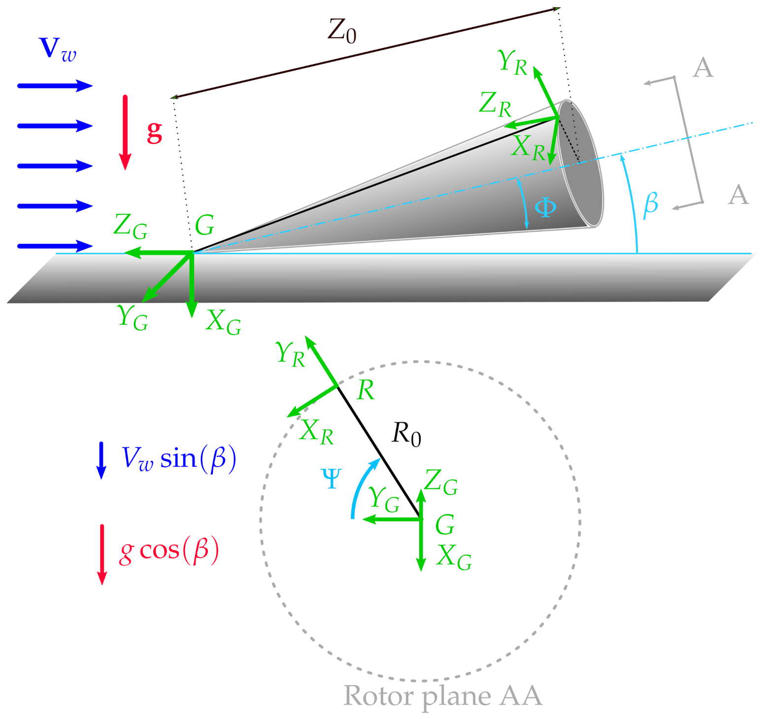
The relative positioning of the lifting surfaces, as well as the inertia matrix of the craft, are typically given in a reference system attached to the AWES, which does not depend on the operational regime and might be centered in principle in any point of the aircraft. This coordinate system is called here body coordinate system ${\mathcal{F}}_B$. In Table 13, data of the lifting surfaces, and similarly the elements of the inertia matrix, are assigned in this coordinate system. To express the geometrical and inertial quantities given in ${\mathcal{F}}_B$ into ${\mathcal{F}}_S$, where the equations have been written, ${\theta }_{BS}$ is defined as the angle around the $Y_B$ axis which describes a rotation from ${\mathcal{F}}_B$ to ${\mathcal{F}}_S$. A graphical representation of ${\mathcal{F}}_B$ and ${\mathcal{F}}_S$ is given in Figure 8, highlighting two possible flight conditions. Finally, the wind velocity and the elevation angle describe the operational regime.

Once the inputs are defined in LT-GliDe, the trim condition is computed. In particular, the turning radius $R_0$, the kite velocity $u_0$, the tether strain and the lifting properties of the control surfaces describe the trim condition. Algorithm 1 is used to find the trim condition for an AWES flying the circular path.

Algorithm 1: Algorithm for the trim evaluation.

The code is such that five different cases of increasing complexity can be analyzed. In

Table 14. Flight options in LT-GliDe.

Case	Motion		Wind		Tether
a	Straight	$R_0\to \infty$	off	$G\to \infty$, $u_0$ imposed	off	$\beta =\frac{\pi }{2}$
b	Straight	$R_0\to \infty$	off	$G\to \infty$, $u_0$ imposed	on
c	Straight	$R_0\to \infty$	on		on	$\beta <\frac{\pi }{2}$
d	Circular		off	$G\to \infty$, $u_0$ imposed	on
e	Circular		on		on	$\beta <\frac{\pi }{2}$

they are summarized. Results from the five cases are introduced, so that complexity is incrementally increased and they can be compared. Case a models the motion of an aircraft in steady and leveled flight without tether (this is basically a standard aircraft in steady, horizontal flight). Case b models the motion of a tethered AWES in a straight motion, with an imposed velocity. Case c models the motion of a tethered AWES in a straight crosswind motion. Case d models the motion of a tethered AWES in a circular motion, with an imposed velocity. Case e models the motion of a tethered AWES in a circular crosswind motion.

Once the trimmed condition has been computed, the linearized dynamics are populated and the eigenproblem can be studied. The eigenvectors of the linearized system give information about its eigendynamics, while the eigenvalues provide a crucial information on the stability of the system.

5. Model Validation

5.1. Eigenproblem Validation

To validate the problem formulation, an ultralight glider named Zefiro, designed internally at the Department of Aerospace Science and Technology of the Politecnico di Milano [20], has been considered. This aircraft has been selected because it is expected to have similar characteristics to AWESs, in term of mass properties and flight dynamics for straight and leveled flight, as per available internal studies and reports. The geometry and mass properties necessary for this study are given in

Table 15. Geometry and mass properties of the ultralight aircraft Zefiro. The tether attachment position has been arbitrarily picked.

Main Wing		Horizontal Tail		Vertical Tail		Geometry		Mass
A	14.25 m${}^2$	A	1.1 m${}^2$	A	1.49 m${}^2$	${\mathbf{X}}_{0CG}^b$	[0,0,0]’ m	m	530 kg
b	15.18 m	b	2.44 m	b	1.6 m	${\mathbf{X}}_{0W}^b$	[0.25,0,0]’ m	$I_{xx}^b$	2104 kg m${}^2$
$C_{D0}$	0.0176	$C_{D0}$	0.0176	$C_{D0}$	0.0176	${\mathbf{X}}_{0H}^b$	[−4,0,0]’ m	$I_{yy}^b$	1122 kg m${}^2$
$\Gamma$	−5${}^{\circ }$					${\mathbf{X}}_{0V}^b$	[−4,0,0]’ m	$I_{zz}^b$	3134 kg m${}^2$
$\Lambda$	5${}^{\circ }$					${\mathbf{X}}_{0T}^b$	[−0.2,0,0]’ m	$I_{xz}^b$	91 kg m${}^2$

. Zefiro features $-5^{\circ }$ of dihedral angle and $5^{\circ }$ of sweep.

Once all the derivatives of external forces are evaluated and the linearized problem populated (Equation (32)), the eigenvalues can be computed and the system stability studied. To check the correct implementation of the equations of motion, the eigenfrequencies of short period, phugoid and Dutch roll are compared with values predicted by the models presented in [21], finding a good agreement. In

Table 16. Eigenfrequencies (rad/s) and damping ratios computed with different formulation.

Model	Short Period		Phugoid		Dutch Roll
	${\omega }_n$	$\zeta$	${\omega }_n$	$\zeta$	${\omega }_n$	$\zeta$
LT-GliDe	12.6	0.46	0.11	0.26	7.35	0.13
Reduced LT-GliDe	9.58	0.60	0.11	0.26	5.21	0.18
Stevens [21]	9.83	0.59	0.20	0.28	5.14	0.19

the eigenfrequencies and damping ratios computed with the different methods are shown for a velocity of 80 m/s.

In the Reduced LT-GliDe model, the computation of the eigenvalues is performed by considering the same state variables as the approximated analytical formulation of Stevens [21]. The values found in this case are indeed more similar to the values found with the analytical formulations.

5.2. Aerodynamic Derivatives Validation

To validate the aerodynamic derivatives analytically derived as shown in the previous part of the paper, the computed values have been compared with the outcome of TORNADO [22], a vortex lattice method.

In order to make TORNADO model the same aerodynamic problem, the MATLAB^® optimization function fmincon, with sqp algorithm, is used to impose the same lift coefficients in the lifting surfaces. In TORNADO, real airfoil data are used to model the wing and tail. Only the lifting surfaces are modelled and the fuselage is left out. The inflow is set to consider both atmospheric wind speed and aircraft motion. To be consistent with the analytic formulation, the drag coefficient at zero lift $C_{D0}$ is included in the drag evaluation. The external forces derivatives are finally obtained by finite difference. In the optimization function, the pitch angle of each lifting surface (main wing and tails) and the ailerons deflection are included as design variables. The square of the difference between the lift coefficients found in LT-GliDe with Algorithm 1 and the lifting coefficients found in TORNADO by pitching the wings is included as objective function. Once the optimization converges (i.e., the two software model the same trim condition), the aerodynamic derivatives can be compared and used to study the eigenvalue problem.

The validation of the derivatives has been performed considering one element a time (e.g. only the main wing or only the vertical tail) and the full aircraft. In this way, the derivatives can be checked individually.

Moreover, the cases introduced in Table 14 can be analyzed in a sequential way, such that different terms in the derivatives can be studied. For example, $\frac{\partial {\mathbf{f}}^w}{\partial \tilde{u}}$ (Equation (56)) can be understood and expressed for the five cases as follow

• $\frac{\partial {\mathbf{f}}^w}{\partial \tilde{u}}=2{\mathbf{P}}_{\mathbf{A}}{\mathbf{C}}_{R0}$ for a straight motion without wind (case a & b)
• $\frac{\partial {\mathbf{f}}^w}{\partial \tilde{u}}={\mathbf{P}}_{\mathbf{A}}\left(2{\mathbf{C}}_{R0}-\frac{{\mathbf{C}}_{\eta }}{G}\right)$ for a straight motion with wind (case c)
• $\frac{\partial {\mathbf{f}}^w}{\partial \tilde{u}}=2\left({\mathbf{P}}_{\mathbf{A}}+{\mathbf{D}}_{\eta \eta }\right){\mathbf{C}}_{R0}$ for a circular motion without wind (case d)
• $\frac{\partial {\mathbf{f}}^w}{\partial \tilde{u}}={\mathbf{P}}_{\mathbf{A}}\left(2{\mathbf{C}}_{R0}-\frac{{\mathbf{C}}_{\eta }}{G}\right)+2{\mathbf{D}}_{\eta \eta }\left({\mathbf{C}}_{R0}-\frac{{\mathbf{C}}_{\eta }}{G}+\frac{{\mathbf{C}}_{L\alpha }}{G}\right)$ for a circular motion with wind (case e)

In

Table 17. Eigenvalues found with the analytical approach (LT-GliDe) and with the vortex lattice method (VLM) in the circular motion case with wind (case e) for different values of sweep and dihedral angle.

$\Gamma =-5^{\circ }$	LT-GliDe	$-29.69$	$-5.75\pm 13.69i$	$-1.05\pm 7.66i$	$-0.20\pm 3.65i$	$-0.01\pm 0.73i$	$-0.17\pm 0.08$
$\Lambda =+5^{\circ }$	VLM	$-24.66$	$-5.41\pm 13.33i$	$-0.98\pm 7.18i$	$-0.23\pm 3.60i$	$0.00\pm 0.75i$	$-0.20\pm 0.09$
$\Gamma =-{10}^{\circ }$	LT-GliDe	$-30.88$	$-5.92\pm 14.85i$	$-0.73\pm 7.72i$	$-0.20\pm 4.15i$	$0.01\pm 0.78i$	$-0.20\pm 0.02$
$\Lambda =+5^{\circ }$	VLM	$-25.13$	$-5.53\pm 14.52i$	$-0.60\pm 7.24i$	$-0.26\pm 4.16i$	$0.01\pm 0.80i$	$-0.21\pm 0.02$
$\Gamma =-5^{\circ }$	LT-GliDe	$-28.29$	$-6.27\pm 17.36i$	$-0.96\pm 7.49i$	$0.05\pm 5.04i$	$0.00\pm 0.73i$	$-0.15$    $-0.10$
$\Lambda =+{10}^{\circ }$	VLM	$-22.68$	$-5.92\pm 17.17i$	$-0.91\pm 7.07i$	$0.01\pm 5.06i$	$0.00\pm 0.74i$	$-0.16$    $-0.11$

, the eigenvalues for Zefiro in the circular motion case with wind at 8 m/s (case e), obtained with TORNADO and with LT-GliDe, are presented for different values of sweep and dihedral angles. The eigenvalues are considered close enough, so that the analytical models for the derivatives in LT-GliDe can be considered a good approximation of the vortex lattice solution of TORNADO.

Both the analytical approach introduced in this paper and the numerical one based on TORNADO can be used to estimate the aerodynamic derivatives of the aircraft. Once the aerodynamic derivatives are estimated (with one of the two methods), derivatives related to the tether and gravity, computed analytically, can be added to formulate the linearize problem and study the eigenproblem associated to the AWES dynamics. The advantage of the analytical approach is the negligible computational cost and the possibility of understanding analytically the relationship between design parameters and stability, which may turn particularly useful in a preliminary design phase where the configuration and geometry of the flying craft are still not frozen. The advantage of a numerical approach is the possibility to model any geometry. The two approaches are therefore to be seen as complementary: the analytical approach will be useful for physical understanding, preliminary design and optimization, while the numerical approach for the detailed aerodynamic design.

6. Results

The results introduced here are meant to show the potential of the proposed approach. A detailed analysis of a AWES designed for power generation is left to future works. In

Table 18. Operational regime characteristics and eigenvalues for the straight motion cases.

Case	a	b	c
$V_w$	-	-	8
G	∞	∞	9.96
$u_0$	80	80	79.67
$\beta$	${90}^{\circ }$	0	0
${\epsilon }_0$	-	6.1 mm/m	6.0 mm/m
Short period	$-5.7830\pm 11.2040i$	$-5.5883\pm 13.3645i$	$-5.7970\pm 13.8910i$
Phugoid	$-0.0275\pm 0.1039i$	$-0.1746\pm 2.6180i$	$-0.1755\pm 3.0697i$
Loyd	0	$-0.2786$	$-0.1358$
Spiral / Pendulum	$-0.0025$	$-0.0639\pm 0.4652i$	$-0.0811\pm 0.4617i$
Dutch roll	$-0.9286\pm 7.2878i$	$-1.0884\pm 7.7242i$	$-1.0660\pm 7.6339i$
Roll sub.	$-29.4738$	$-29.0046$	$-29.7689$

and

Table 19. Operational regime characteristics and eigenvalues for the circular motion case.

Case	a	d	e
$V_w$	-	-	8
G	∞	∞	9.94
$u_0$	80	80	79.5
$\beta$	${90}^{\circ }$	0	0
$\Phi$	-	23.2${}^{\circ }$	23.3${}^{\circ }$
${\epsilon }_0$	-	6.6 mm/m	6.5 mm/m
Short period	$-5.7830\pm 11.2040i$	$-5.5643\pm 13.1730i$	$-5.7535\pm 13.6858i$
Phugoid	$-0.0275\pm 0.1039i$	$-0.1493\pm 3.3064i$	$-0.1979\pm 3.6480i$
Loyd	0	$-0.2117$	$-0.1740\pm 0.0776i$
Spiral	$-0.0025$	$-0.3444$
Pendulum	0	$-0.0018\pm 0.7093i$	$-0.0052\pm 0.7318i$
Dutch roll	$-0.9286\pm 7.2878i$	$-1.0701\pm 7.7724i$	$-1.0481\pm 7.6643i$
Roll sub.	$-29.4738$	$-28.9837$	$-29.6862$

, the eigenvalues for the five cases are reported and linked to each other. The straight and circular motion cases are analyzed in the following sections.

6.1. Case a

This case models the straight and leveled flight of a conventional aircraft. No novelty is introduced in this case, as the tether is not present in the model and the aircraft is flying straight. Conventional longitudinal and lateral modes can be found. A lift coefficient of the main wing of 0.09 is found at a velocity of 80 m/s. The aircraft is longitudinally stable, with a static margin of 20.3 %. For a conventional aircraft, eight eigenvalues are found. Typically, the longitudinal motion can be described by four state variables ($\tilde{u},\tilde{w},\tilde{q},\theta$), which correspond to four eigenvalues: two pair of complex conjugate eigenvalues describing the so-called short period and the phugoid modes. The lateral-directional motion can be described by four state variables ($\tilde{v},\tilde{p},\tilde{r},\varphi$), and it is typically characterized by a pair of complex conjugate (Dutch roll) and two real eigenvalues (spiral and roll subsidence mode).

6.2. Case b and c

For these cases, the tether is added and the mean elevation angle is set to zero, such that gravity is not influencing the results. The considered tether has a diameter of $d_t=1$ cm, the total length at rest is $L_t^0=400$ m, the drag coefficient $C_{\perp }=0.8$ and the Young modulus $E=110$ GPa. The linear spring constant associated to the tether is $\kappa =A_{t}E/L_t^0=21\mathrm{kN}/\mathrm{m}$. The lift coefficient of the main wing is set to 0.9. Since the tether is part of the modelling, two new eigenvalues are expected, related to the position state variables ${\tilde{y}}_{rs}$ and ${\tilde{z}}_{rs}$. The motion is straight, thus the longitudinal and lateral motions can be studied separately.

In Table 18, the eigenvalues of case b and c are reported and associated with the eigenvalues of the airplane mode case. Eigenvalues and eigenmodes trends are consistent for the two cases, so that they are analyzed here together.

Figure 9 shows the longitudinal eigevalues for an increasing tether stiffness for case b. For $E\to 0$, the tether deformation $\epsilon$ goes to infinity to produce enough force on the tether to balance the aerodynamic forces. As in this case the elastic effects are negligible, the tether force is a constant force applied on the tether attachment. This force could be understood as a gravitational force applied on the tether attachment and not on the center of mass.

As the elasticity grows, the short period increases the imaginary part. By performing the same plot for $\kappa =\left(A_{t}E\right)/L_t^0\to \infty$, it is found that the short period has a vertical asymptote corresponding to the eigenmode of the system spring-mass with the elasticity from the tether and the mass from the kite. The phugoid increases its real part till approximately $\kappa \approx 4$ kN/m and later decreases it. A new real longitudinal eigenmode starts from zero and moves in the real axis in the negative direction. In this paper, this eigenmode is called Loyd mode, after Miles L. Loyd, who derived the first power equation of AWESs [23]. The Loyd eigenvalues collapse at very low tether stiffness to a value, suggesting that this mode is not influenced by the tether elasticity.

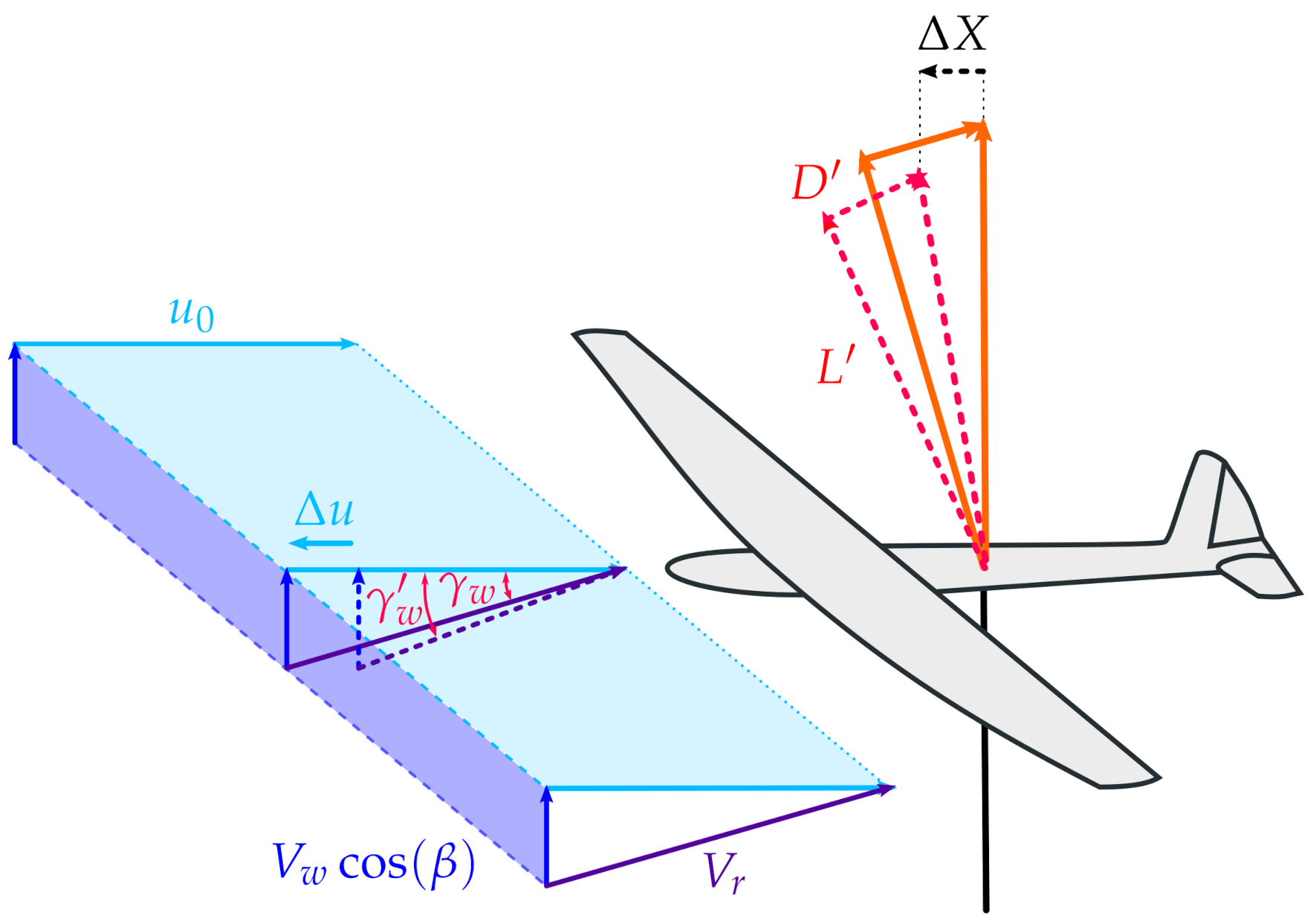
The Loyd mode involves mainly the longitudinal velocity $\tilde{u}$. For AWESs, the longitudinal velocity in equilibrium is given by the balance of the projection of lift along the $X_S$ axis and drag. When $\tilde{u}$ is perturbed, the kite tends to go back to the equilibrium point. A graphical representation of this mode is given in Figure 10. In the figure, the AWES velocity is decreased of $\Delta u$, such that the inflow angle ${\gamma }_w$ is increased with respect to the steady state value (${\gamma }_w^{\prime }>{\gamma }_w$). Lift is perpendicular to the relative wind speed and a positive force $\Delta X$ along the $X_S$ axis is generated. This force acts to restore the equilibrium condition.

The eigenmode can be approximated by a simple first order differential equation in the general form $\tilde{\dot{u}}=\tilde{\mathbf{A}}(1,1)\tilde{u}$, such that the associated eigenvalue is

$$\begin{array}{cc}\hfill {\lambda }_L& \approx \left(\frac{C_L}{G}-2C_D-\frac{C_{D\alpha }}{G}-2C_{\perp }\frac{d_t{L}_t^0}{4A}\right)\frac{\frac{1}{2}\rho A{u}_0}{m},\hfill \end{array}$$

(85)

where the aerodynamic coefficients are related to the full flying craft. For the case with no wind (case b), $G\to \infty$, then

$$\begin{array}{cc}\hfill {\lambda }_L{|}_b& \approx -2\left(C_D+C_{\perp }\frac{d_t{L}_t^0}{4A}\right)\frac{\frac{1}{2}\rho A{u}_0}{m}.\hfill \end{array}$$

(86)

For the straight motion case with wind (cases c), $G=\frac{C_L}{C_D+C_{\perp }\frac{d_t{L}_t^0}{4A}}$, then

$$\begin{array}{cc}\hfill {\lambda }_L{|}_c& \approx -\left(C_D+\frac{C_{D\alpha }}{G}+C_{\perp }\frac{d_t{L}_t^0}{4A}\right)\frac{\frac{1}{2}\rho A{u}_0}{m}.\hfill \end{array}$$

(87)

This approximation suggests that for a well designed AWES this eigenvalue is always real and negative, as the term inside the brackets in Equations (86) and (87) is positive.

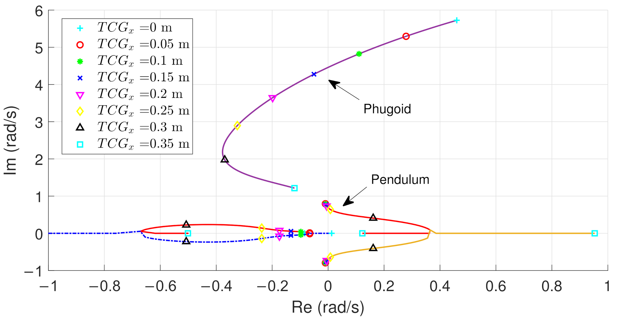
To better characterize the longitudinal modes, the eigenvalues are tracked as function of the tether attachment position along the $X_S$ axis. Figure 11 shows the longitudinal eigenvalues for an increasing distance between the tether attachment and the center of mass. When $TC{G}_x=0$ m, the two points coincide, while when $TC{G}_x=0.2$ m (nominal value considered in the paper), the tether attachment is placed 20 cm aft. Interestingly, the phugoid for high $TC{G}_x$ collapses to two real eigenmodes, one of which moves along the real positive axis. The Loyd eigenvalue is basically fixed at low $TC{G}_x$ and it drastically decreases its real part approximately when the phugoid becomes unstable.

Figure 12 shows two lateral eigenvalues as functions of the tether stiffness. The lateral mode related to Dutch roll and to roll subsidence are basically not influenced by the tether stiffness, then they are left out of the plot. The spiral mode increases its real part until matching another lateral eigenvalue on the real axis. After the two coalesce, they become complex conjugates for further values of the parameter. The coalescence happens at really low stiffness values ($\kappa \approx 0$ kN/m), and the eigenvalues collapse rapidly to a location, suggesting that this mode is not influenced by the tether elasticity. The eigenvalues for $\kappa >0$ kN/m have the imaginary part much larger than the real part, suggesting that this mode is lightly damped. This new oscillating stable mode is dominated by a linear lateral motion (involving ${\tilde{y}}_{rs}$), and small perturbations in $\varphi$ and $\psi$ and it is called here pendulum mode. Its natural frequency is ${\omega }_n=0.47$ rad/s (case c).

By considering a pendulum composed by the tether and a kite subject to aerodynamic force, the oscillation frequency is ${\omega }_{pend}=\sqrt{\frac{T}{m{L}_{t0}}}$, where T is the tether force, m is the kite mass and $L_{t0}$ is the tether length. The frequencies found in this simplified way is ${\omega }_{pend}=0.49$ rad/s (case c), close to what has been found in the LT-GliDe analysis.

By modifying the dihedral angle, while keeping the main wing aerodynamic center fixed to isolate the effect of the change, to $\Gamma =0^{\circ }$, the pendulum mode becomes unstable: ${\lambda }_p=0.04\pm 0.47$. If it is modified to $\Gamma =-{10}^{\circ }$, the real part becomes more and more negative: ${\lambda }_p=-0.19\pm 0.42$. Dihedral angle then largely influences the real part of the pendulum mode and should be considered to achieve stability. The spiral mode, for conventional aircrafts, depends on the dihedral angle: so does the pendulum mode for AWESs, which arises from it (Figure 12).

6.3. Case d

The circular motion is now considered. In this case, the inflow varies along the main wing and ailerons are used to trim the aircraft. In particular, it is assumed that ailerons deflections do not influence the section drag coefficient (i.e., $\Delta C_D=0$). Longitudinal and lateral modes cannot be separated and they shall be studied together. However, by looking at the numerical values in Table 19, short period, Dutch roll and roll subsidence have consistent values with the straight motion cases.

Figure 13 shows all the non-zero eigenvalues (apart from the roll subsidence) for the circular motion without wind (case d).

The pendulum mode is represented by a pair of complex conjugate eigenvalues starting from the origin. For $\kappa >1$ kN/m, all points have the same value, suggesting that this mode is not influenced by the tether elasticity. The spiral mode eigenvalue moves along the real axis. For extremely low $\kappa$ it moves towards the negative direction, and for $\kappa \approx 2$ kN/m it starts increasing in its real part again. It is basically not influenced by the tether stiffness. The Loyd mode decreases its real part as in the straight motion case and from low tether stiffness its eigenvalues are fixed to the same value.

6.4. Case e

In case e the wind velocity is considered and the kite speed is computed from the force balance. Similar to the previous cases, in Figure 14 the eigenvalues are tracked for an increasing tether stiffness. Only the modes typical of AWESs are shown in figure. Interestingly, Loyd and spiral modes are coalescing and merging into a pair of complex conjugate eigenvalues. The corresponding mode is called positional mode in the paper. The positional mode is not influenced by tether stiffness, as for low values of rigidity the eigenvalues have the same value.

In Figure 15, the eigenvalues are tracked as functions of the tether attachment position. The Loyd and the spiral mode for an increasing distance between the center of mass and tether collapse to a pair of complex conjugate eigenvalues (positional mode). This new oscillating mode is stable and highly damped. By increasing again $TC{G}_x$, the positional mode splits again in two real eigenvalues.

The phugoid is also largely influenced by the tether attachment position. For $TC{G}_x=0$ m, this mode is unstable, while when moving the tether attachment aft, its real part gets negative.

The pendulum mode eigenvalue displays instead an opposite trend. While moving the tether attachment aft, its real part becomes positive and finally the two pairs of complex conjugate eigenvalues become two real and positive eigenvalues. For the straight motion case (Figure 11), for high $TC{G}_x$ the phugoid splits into two real eigenvalues, while for the circular motion case the pendulum splits instead. This suggests that, when designing the AWES for stability, the circular motion case with wind shall be considered to properly characterize the eigendynamics of the system: even if some of the eigenvalues for straight and circular motion are similar for some specific cases, trends over the full design space might change radically.

This analysis highlights the importance of carefully choosing the tether attachment position when designing for stability.

7. Conclusions

This paper introduces a methodology to study the flight stability of rigid wing Airborne Wind Energy Systems (AWESs). A fictitious steady state motion of the kite in a circular path is found by considering all fluctuating terms during the loop, such as gravity and aerodynamic forces related to the mean elevation angle, as disturbances. The selected circular path is characterized by a turning radius which makes the force on the tether to be maximized. Once the steady state is found, all derivatives of external forces are computed to formulate the linearized dynamics, and the flight stability can be studied from the ensuing model. As the fictitious steady state is representative of the flight over the loop, flight dynamic performances and control efforts are expected to benefit from a stable design.

The steady state forces and the aerodynamic derivatives are computed using an analytical approach. The computational cost of the linearized problem evaluation is negligible compared to other methods, which make this tool suitable for a preliminary design phase. Moreover, the analytical formulation allows for an intuitive and quantitative understanding of how stability is influenced by design parameters. Indeed, the modelling introduced in this work takes into account all the main design features of AWESs: main wing geometry (position, area, aspect ratio, sweep, dihedral), main wing aerodynamics, control surfaces aerodynamics and geometry (area, aspect ratio, position), tether attachment position, tether mechanical and aerodynamic properties and mass properties of the kite. Moreover, the non-uniform distribution of the inflow along the wing span, due to the rotational velocity of the kite, is also taken into account.

The presence of the tether introduces three new state variables compared to conventional aircraft flight mechanics. However, the variable describing the kite position in the circular path does not influence the linearized dynamics because the problem has been formulated to be axial-symmetric.

The model is implemented in MATLAB^® and the suite has been named LT-GliDe (Linearized Tethered Gliding system Dynamics). LT-GliDe is a module of an under-development multidisciplinary design and optimization framework for rigid wing AWESs, named T-GliDe (Tethered Gliding system Design). Five cases of increasing complexity can be studied: AWES operating in aircraft mode (without tether), AWES operating in tethered straight motion without wind, AWES operating in tethered straight crosswind motion, AWES operating in tethered circular motion without wind, AWES operating in tethered circular crosswind motion.

The aerodynamic analytical derivatives have been validated using vortex lattice method (TORNADO) and an internally-designed glider, called Zefiro, is used to validate the problem formulation for straight and leveled flight. Zefiro is then used as an example to show the features of this modelling approach. A tether is attached to Zefiro in a position such that all eigenvalues have a negative real part for the tethered circular crosswind motion case. The five cases are finally analyzed.

In straight tethered motion, longitudinal and lateral motion can be decoupled. Ten non-null eigenvalues are found, two more than a conventional aircraft in steady and leveled flight. It has been shown how the tether modifies the conventional eigenmodes and the physics of two new modes is explained. The Loyd mode is a mode typical of AWESs, which brings the kite back to the equilibrium longitudinal velocity after a perturbation. The pendulum mode arises by the merge of a new mode with the spiral mode and has the frequency of a pendulum characterized by the force applied on the tether. Its real part, defining the mode stability, is largely influenced by the main wing dihedral angle.

In circular motion, longitudinal and lateral equations are coupled and so are the eigenmodes. However, short period, Dutch roll and roll subsidence eigenvalues have consistent values with the straight motion cases. Eleven non-null eigenvalues are found in this case, three more than for conventional aircrafts. Two are due to the presence of the tether and one to the steady maneuver. Also in this case, the pendulum mode can be found, as well as the Loyd mode in the case without wind. For the crosswind circular motion case, the Loyd mode merges with the spiral mode to bear a pair of complex conjugate eigenvalues (positional mode).

It is investigated how the tether attachment position influences stability. By moving the tether attachment aft with respect to the center of mass, the phugoid becomes stable and the pendulum mode unstable. The tether attachment location should then be carefully designed to achieve stability of all modes. Flight mechanics should generally be studied with the circular crosswind motion model, as the eigendynamics for this case can be radically different from the more simplified other cases.

As LT-GliDe is suitable for preliminary design and optimization of rigid wing AWESs, it is being included in a system design framework (T-GliDe) and optimal designs will be analyzed in future works. It is expected that an aircraft designed with this approach will reduce control action and the need for control authority. Aero-elastic time-marching simulations are envisaged to study the eigenmodes and the controllability with higher fidelity codes.

References

1. Trevisi, F.; Gaunaa, M.; Mcwilliam, M. Configuration optimization and global sensitivity analysis of Ground-Gen and Fly-Gen Airborne Wind Energy Systems. Renew. Energy RENE 2021, 178, 385–402. [Google Scholar] [CrossRef]
2. Schmehl, R.; Tulloch, O. Airborne Wind Energy Conference 2019: (AWEC 2019); Delft University of Technology: Glasgow, UK, 2019. [Google Scholar]
3. Vermillion, C.; Cobb, M.; Fagiano, L.; Leuthold, R.; Diehl, M.; Smith, R.S.; Wood, T.A.; Rapp, S.; Schmehl, R.; Olinger, D.; et al. Electricity in the air: Insights from two decades of advanced control research and experimental flight testing of airborne wind energy systems. Annu. Rev. Control 2021. ISSN 1367-5788. [Google Scholar] [CrossRef]
4. Makani Power. Available online: https://makanipower.com/ (accessed on 21 June 2021).
5. KiteKraft. Available online: https://kitekraft.de/ (accessed on 21 June 2021).
6. EnerKite. Available online: https://www.enerkite.de/en/ (accessed on 21 June 2021).
7. KITEPOWER. Available online: https://kitepower.nl/ (accessed on 21 June 2021).
8. Ampyx Power. Available online: https://ampyxpower.com/ (accessed on 21 June 2021).
9. TwinTec. Available online: http://twingtec.ch/ (accessed on 21 June 2021).
10. KiteMill. Available online: http://www.kitemill.com/ (accessed on 21 June 2021).
11. Homsy, G. Oktoberkite and the MX2. In The Energy Kite Part I; Echeverri, P., Fricke, T., Homsy, G., Tucker, N., Eds.; Makani Technologies LLC: Alameda, CA, USA, 2020; pp. 7–89. [Google Scholar]
12. Sicard, J.; Homsy, G.; Abraham, M. Kite Stability in Crosswind Flight. In The Energy Kite Part II; Makani Technologies LLC: Alameda, CA, USA, 2020; pp. 223–232. [Google Scholar]
13. Terink, E.J.; Breukels, J.; Schmehl, R.; Ockels, W.J. Flight Dynamics and Stability of a Tethered Inflatable Kiteplane. J. Aircr. 2011, 48, 503–513. [Google Scholar] [CrossRef]
14. Salord Losantos, L.; Sánchez-Arriaga, G. Flight Dynamics and Stability of Kites in Steady and Unsteady Wind Conditions. J. Aircr. 2015, 52, 660–666. [Google Scholar] [CrossRef] [Green Version]
15. Pastor-Rodríguez, A.; Sánchez-Arriaga, G.; Sanjurjo-Rivo, M. Modeling and Stability Analysis of Tethered Kites at High Altitudes. J. Guid. Control. Dyn. 2017, 40, 1892–1901. [Google Scholar] [CrossRef]
16. Trevisi, F.; Gaunaa, M.; Mcwilliam, M. The Influence of Tether Sag on Airborne Wind Energy Generation. J. Phys. Conf. Ser. 2020, 1618, 032006. [Google Scholar] [CrossRef]
17. Gaunaa, M.; Forsting, A.R.M.; Trevisi, F. An engineering model for the induction of crosswind kite power systems. J. Phys. Conf. Ser. 2020, 1618, 032010. [Google Scholar] [CrossRef]
18. Nelson, R.C. Flight Stability and Automatic Control, 2nd ed.; McGraw-Hill: New York, NY, USA, 1998. [Google Scholar]
19. Phillips, W.F.; Anderson, E.A.; Jenkins, J.C.; Sunouchi, S. Estimating the Low-Speed Downwash Angle on an Aft Tail. J. Aircr. 2002, 39, 600–608. [Google Scholar] [CrossRef]
20. Department of Aerospace Science and Technology (DAER), Politecnico di Milano. Via La Masa, 34, 20156 Milano-Italy. Available online: https://www.aero.polimi.it/ (accessed on 21 June 2021).
21. Stevens, B.L.; Lewis, F.L. Aircraft Control and Simulation; John Wiley: Hoboken, NJ, USA, 2003. [Google Scholar]
22. Melin, T. User’s Guide and Reference Manual for Tornado. Available online: https://tornado.redhammer.se/index.php (accessed on 21 June 2021).
23. Loyd, M.L. Crosswind Kite Power. J. Energy 1980, 4, 106–111. [Google Scholar] [CrossRef]
Figure 1. General procedure for the stability analysis of rigid wing AWESs.
Energies 14 07704 g001
Figure 2. Ground coordinate system F G and rotating coordinate system F R .
Energies 14 07704 g002
Figure 3. Rotating coordinate system F R and stability coordinate systems F S . On the left, a graphical representation of the three sequential planar rotations from F R to F S . As angles ϕ , θ and ψ are assumed to be small and R R S R is linearized about the condition ϕ = θ = ψ = 0 , they can be interpreted as rotation angles about axes X R , Y R and Z R , which is shown on the right.
Energies 14 07704 g003
Figure 4. Right wing coordinate system F W r and stability coordinate system F S .
Energies 14 07704 g004
Figure 5. Velocity triangle and aerodynamic forces for the main wing.
Energies 14 07704 g005
Figure 6. Symmetrical ailerons deflection.
Energies 14 07704 g006
Figure 7. Main forces acting along the Y S axis. The vertical tail is stabilizing the effect of the centrifugal forces.
Energies 14 07704 g007
Figure 8. Body reference frame F B and stability reference frame F S for a case with negative θ B S (a) and positive θ B S (b).
Energies 14 07704 g008
Figure 9. Longitudinal eigenvalues for an increasing tether stiffness for case b. The top-right box displays the area close to the origin.
Energies 14 07704 g009
Figure 10. Graphical representation of the Loyd mode.
Energies 14 07704 g010
Figure 11. Longitudinal eigenvalues as function of the tether attachment position for case c. The short period is not shown.
Energies 14 07704 g011
Figure 12. Two lateral eigenvalues for an increasing tether stiffness for the case b.
Energies 14 07704 g012
Figure 13. Eigenvalues for an increasing tether stiffness for case d. On the top plot, all eigenvalues, apart roll subsidence, are shown. On the bottom, the eigenvalues close the origin are displayed.
Energies 14 07704 g013
Figure 14. Eigenvalues for an increasing tether stiffness for case e.
Energies 14 07704 g014
Figure 15. Sensitivity of the eigenmodes with respect to the tether attachment position along the X S axis for case e.
Energies 14 07704 g015