The Elephant Problem—Determining Bulk Thermal Diffusivity

Abstract

This study investigates a measurement method of thermal diffusivity for samples with arbitrary geometries and unknown material properties. The aim is to curve fit the thermal diffusivity with the use of a numerical simulation and transient temperature measurement inside the object of interest. This approach is designed to assess bulk material properties of an object that has a composite material structure such as underground soil. The method creates the boundary conditions necessary to apply analytical theory found in the literature. It was found that measurements best correlated with theory and simulation at positions between the center and surface of an object.

1. Introduction

Underground soil for thermal energy storage is becoming more common as it is abundant and a viable storage media. The earth consists of at least two phases, consisting of materials that have very different thermal properties (e.g., humid earth, gravel, and air). The properties of the underground need to be determined to properly design seasonal underground thermal storages. Bore probe samples of underground are composed of inhomogeneous materials and mean soil property values are needed for the analysis and design of the storage performance.

The use of analytical instruments to measure mean property values (e.g., thermal conductivity) of such geological probes is quite complex owing to the geometry and nature of the samples. Geological probes are extracted with rotary drilling equipment, rendering cylindrical samples. Owing to the finite length of drill rods (<3 m), only sections of earth can be obtained, and they are often fractured or broken during the process of extraction [1]. Extending the theory of heat conduction in solids to measure thermal conductivity requires subjective assumptions treating samples as homogenous materials with uniform water distribution, perfect contact with the measurement device, and no migration of moisture during measurement [2].

There are two categories of state-of-the art measurement methods (steady-state and transient) for thermal conductivity, which is needed to calculate thermal diffusivity. Each method has its own set of advantages and disadvantages in determining thermal conductivity [2,3,4,5,6,7,8,9].

A new method is developed in this work for the determination of thermal diffusivity for a solid sample of arbitrary shape using a combination of a simple experimental temperature measurement in combination with a numerical simulation of a complex geometry and fit of the thermal properties.

To develop the method, first, an analytical and numerical solution are evaluated for a sphere as a well-known geometry using a material with known properties. The definition of a maximum acceptable deviation for thermal diffusivity of 10% is established to constrain the analysis. Second, a simple experiment to employ the necessary boundary conditions to validate the test method and numerical model is designed and developed. The procedure assumes a sufficiently high heat transfer rate of approximately 1000 W/(m·K) over the entire object surface. Finally, tests using an irregular shape (an elephant as a metaphor for sympathy and size of the problem) are analyzed for comparison with the simplified geometry.

2. Materials, Theory, and Methods

2.1. Materials

The material chosen for physical test measurements was polylactic acid (PLA). It was chosen for its low thermal diffusivity, which allowed for a compact test stand and flexibility as a 3D-printable material, i.e., a sphere and an elephant. Materials often used in thermal storages exhibit low thermal diffusivities, making PLA a suitable choice. Tap water was used as the heat transfer fluid in the tank.

Table 1. Thermal properties of materials used in the experimental set-up.

Material	Thermal Conductivity	Specific Heat Capacity	Density
Water	0.629 [W/(m·K)] 1	4178.8 [J/(kg·K)] 1	992.1 [kg/m3] 1
Air	0.0267 [W/(m·K)] 1	1006.7 [J/(kg·K)] 1	1.149 [kg/m3] 1
PLA	0.129 [W/(m·K)] 2	1301.5 [J/(kg·K)] 2	1120.7 [kg/m3] 2
PIR	0.02 [W/(m·K)] 3	n/a	n/a

¹ Referenced from the VDI Heat Atlas @ 40 °C for water, 30 °C for air. ² Determined using in-house measurements. ³ Referenced from Swisspor product label. Thermal diffusivity of PLA 8.8442 × 10⁻⁸ (m²/s) determined from ².

lists the material properties of the materials used. The tank was insulated using Swisspor AG (Boswil, Switzerland) PIR insulation panels. Figure 1 below shows the basic layout of the test stand.

A tank made of 2 mm carbon nickel steel plate was fabricated to contain a fluid bath in which the objects were to be placed for measurement.

2.2. Theory

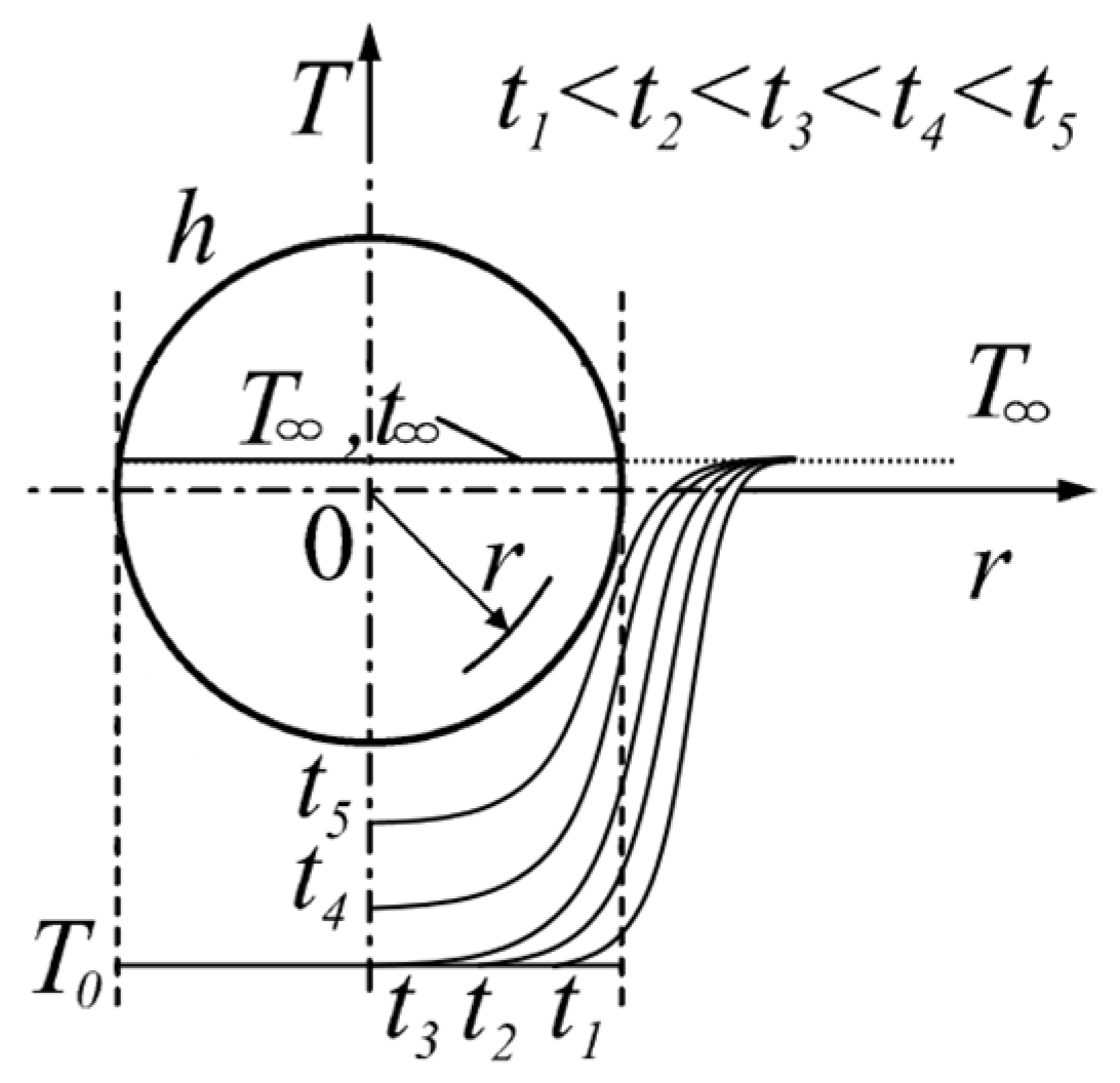
An analytical solution for the transient temperature evolution inside an object exists for a sphere, cylinder, and flat plate [10,11]. Figure 2 below depicts the qualitative temperature change for a cool sphere immersed into a warm fluid.

The x-axis indicates the radial position, and the y-axis indicates temperature. The initial temperature of the sphere before entering the fluid is denoted as ${\mathrm{T}}_0$ and the final temperature as ${\mathrm{T}}_{\infty }$. Profiles ${\mathrm{t}}_1$ to ${\mathrm{t}}_5$ display how the temperature changes as a function of time and radial position within a spherical object.

Temperature profiles are a function of several important boundary conditions. First, a symmetric temperature profile assumes a constant value of high heat transfer over the entire surface of the object. Second, the thermal properties of the object must be considered as well as the characteristics of the fluid flow. Third, geometry has a great influence on the temperature evolution within the object. Figure 3 below illustrates the solution for the transient temperature field as an error function approximated with a series of transcendental functions. The plot below is for the center of a sphere of arbitrary material and heat transfer conditions.

The x-axis represents non-dimensional time and is scaled using the thermal diffusivity $\mathsf{\kappa }$ (m²/s) of the chosen material and scaled by the characteristic length, r (m), i.e., the Fourier number:

$$\mathrm{Fo}=\frac{\mathsf{\kappa }\cdot \mathrm{t}}{{\mathrm{r}}^2}$$

(1)

The y-axis is defined by a non-dimensional temperature representing the fractional temperature change relative to the range defined by the initial temperature of the sphere, ${\mathrm{T}}_0$, and the temperature of the water in the tank, ${\mathrm{T}}_{\infty }$,

$$\mathsf{\Theta }=\frac{\mathsf{\theta }}{{\mathsf{\theta }}_0}=\frac{\mathrm{T}\left(\mathrm{r},\mathrm{t}\right)-{\mathrm{T}}_{\infty }}{{\mathrm{T}}_0-{\mathrm{T}}_{\infty }}$$

(2)

The curves in Figure 3 above represent the evolution of temperature at the center of a sphere, $\mathrm{T}\left(\mathrm{r},\mathrm{t}\right)$, where $\mathrm{r}=0$. They are a family of curves representing the ratio of convective heat transfer at the surface, $\mathrm{h}$ (W/(m²·K)), to the conductive heat transfer, λ (W/(m·K)), inside the object scaled by the characteristic length, e.g., the Biot number for a sphere:

$$\mathrm{Bi}=\frac{\mathrm{h}\cdot \mathrm{r}}{\mathsf{\lambda }}$$

(3)

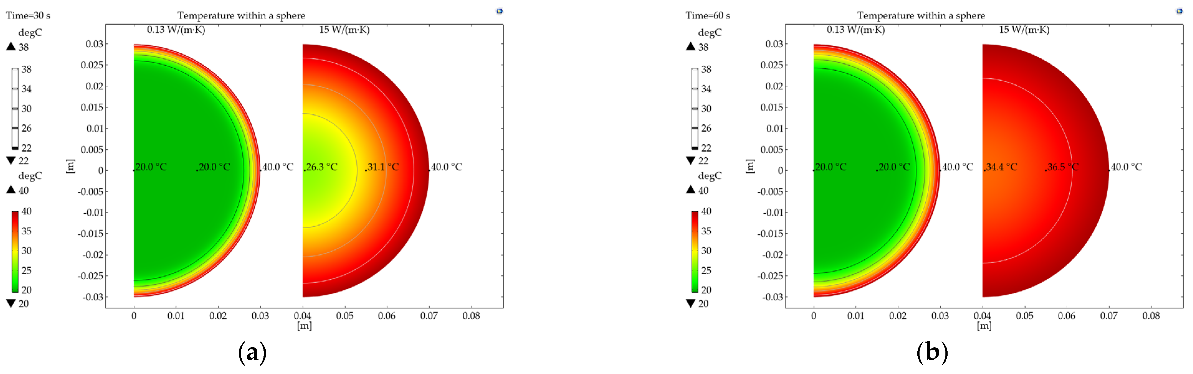
The Biot number determines the transient temperature profile as an object is heated up or cooled down in an immersed fluid. Generally, a Bi ≪ 1 indicates relatively poor convective heat transfer and near uniform temperature within the object (a), whereas a Bi ≫ 1 indicates relatively poor conductive heat transfer and a large temperature gradient within the object. Figure 4 below compares both (a) and (b) scenarios at two different times.

The sphere on the right in both panels represents a metal that experiences a sharp rise in temperature in a very short period. In addition, Figure 3 reveals an exponential approach to the theoretical boundary condition $\mathrm{Bi}=\infty$ with increasing Biot numbers. The roots of the transcendental equation for $\mathrm{Bi}=120$ are approximately 0.83% different from the boundary condition $\mathrm{Bi}=\infty$. A $\mathrm{Bi}\ge 120$ was chosen sufficient to assume this boundary condition for comparison with experimental measurements. Thus, the method in this work relies on high Biot numbers with relative high heat transfer coefficients and the selection of a test material with low conductivity was made to allow for more measurements during the change in temperature.

Geometries of an arbitrary shape take on similarly shaped curves as those found in Figure 3. Analytical functions for the transient temperature evolution for arbitrary geometries do not exist in the literature. A complex surface exhibits a unique set of Biot curves that do not correlate with those of a sphere. Therefore, a numerical simulation is necessary to generate the curves necessary for comparison with the measured results for arbitrary geometries.

2.3. Methods

2.3.1. Procedure

The measurement concept was developed with an experiment to create the boundary conditions necessary for comparison of the measurements with the related theory for the sphere and with a numerical model for the elephant. The numerical model was validated for a sphere also using the analytical theory. All measurements were compared using the ideal boundary condition $\mathrm{Bi}=\infty$. The goal was to measure the elephant and record a position specific temperature over time to determine the thermal diffusivity by comparison with a numerical model.

2.3.2. Physical Experiment

Using the stated materials and related theory, an experiment was developed to determine the average thermal diffusivity of an arbitrary object. The proposed method prescribes the rapid immersion of a test object into a turbulent isothermal fluid.

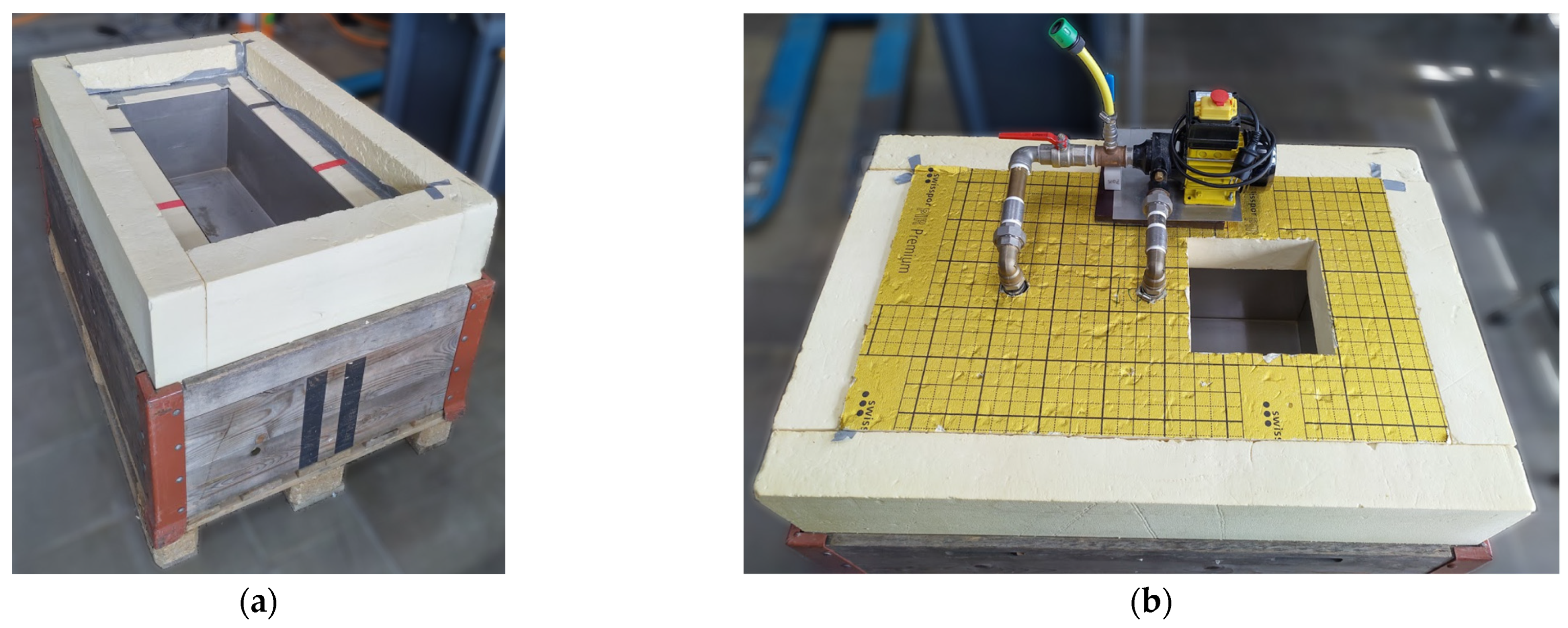
The test stand shown in Figure 5 consists of an insulated steel tank for the purpose of circulating water across the test object via a pump. A quantity of water weighing 60 kg was used to transfer heat to the cooler object without a significant drop or gain in fluid temperature during the test.

A Keysight (Otelfingen, Switzerland) DAQ970A data logger recorded temperature data from calibrated type K, 0.13 mm wire thickness, (∅ = 0.6 mm), PFA-insulated thermocouples (Omega (Norwalk, CT, USA): 5SC-TT-KI-36-2M) for the water temperature and temperature inside the object. A measurement sweep was recorded every ~0.2–0.3 s for approximately 1 h. The velocity of the water was regulated (~0.1 m/s) to create a sufficiently high and constant heat transfer coefficient at the surface of the objects consistent with a Bi > 120 with the given geometry and thermal diffusivity of the test material.

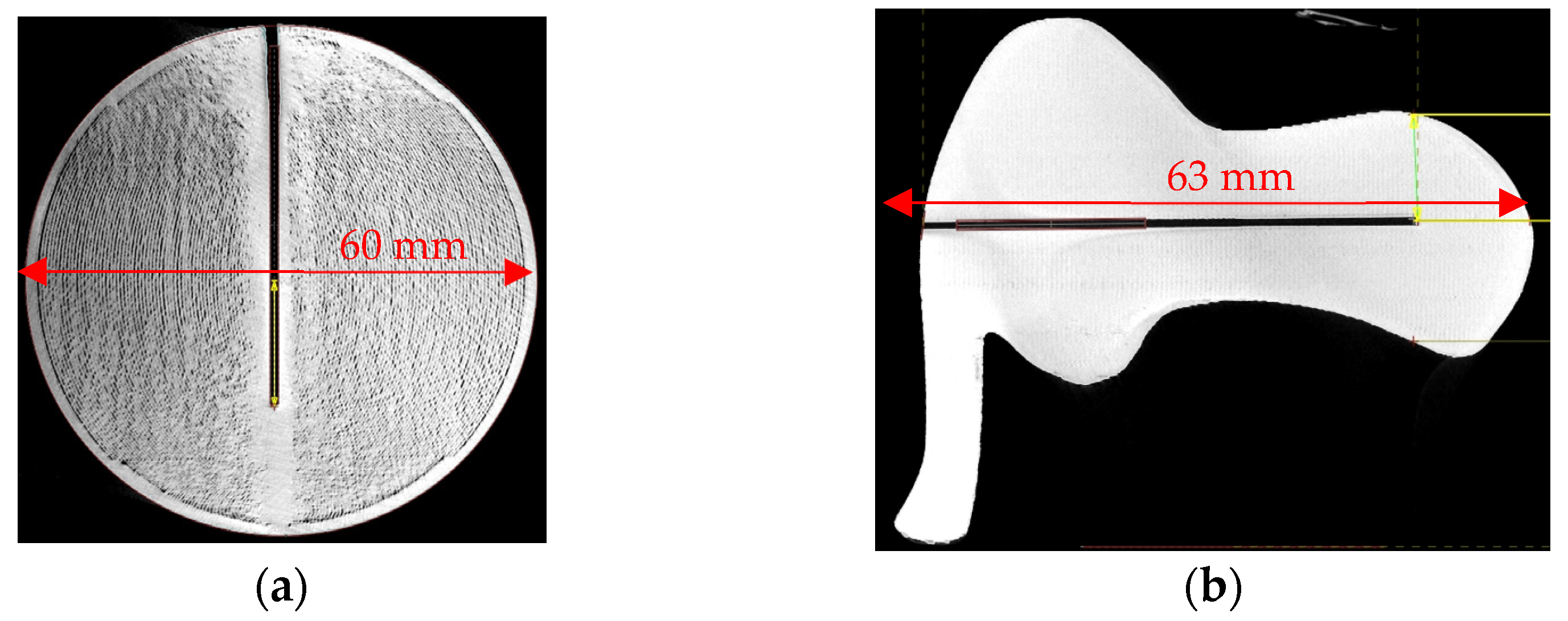
Spheres (∅ = 60 mm) and an elephant (l, w, h = 63 mm × 43 mm × 61 mm) of PLA measuring were 3D-printed using an Ultimaker 3 (Utrecht, The Netherlands). A hole of ~1 mm was drilled to a prescribed internal point to place a thermocouple and measure the internal temperature of the object over time. The calibrated thermocouples were placed in contact with the objects at the end of the drilled hole. Figure 6 shows an example of hole drilled for measurement.

2.3.3. Numerical Simulation

A numerical simulation in COMSOL Multiphysics (Zürich, Switzerland) v5.5 was used to model the temperature evolution of the object placed into the steel tank. The model did not account for the fluid flow. A boundary condition of $\mathrm{Bi}=\infty$ was chosen, where the free temperature of the fluid is assumed to be the surface temperature of the object. A sphere was simulated with a 2D axisymmetric transient simulation for comparison with the analytical theory using a maximum element size of 0.6 mm, consisting of 14,176 elements. After validation, a 3D transient model for the elephant served as the point of comparison with measurement data from the elephant test object with a maximum element size of 6.38 mm, consisting of 29,383 elements. Figure 7 below shows both meshes simulated.

3. Results

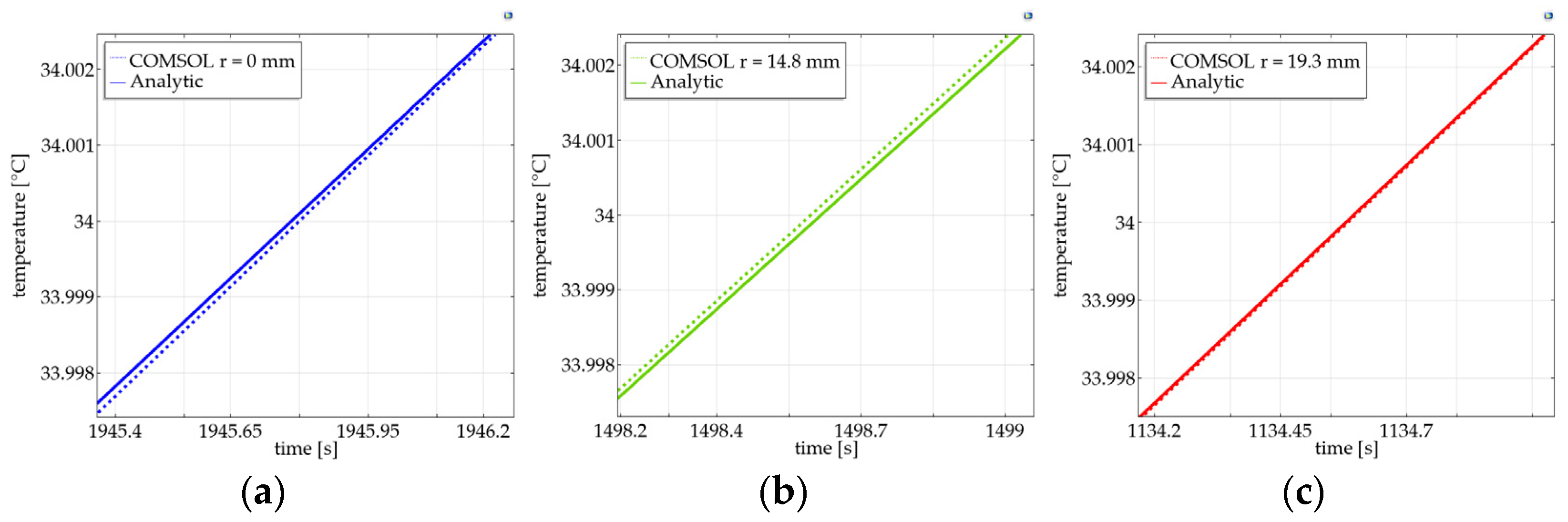
3.1. Validation of COMSOL Simulation and Theory

Effective use of a COMSOL simulation for arbitrary geometries required a model validation with a geometry compatible with the analytical theory. The comparison was made for a sphere at the center (r = 0), r = 14.8 mm, and r =19.3 mm. A sphere of initially 20 °C was exposed to a sudden change of surface temperature of 40 °C. Figure 8 plots the simulated temperatures versus the analytical for a period of 2 h (7200 s).

3.2. Comparison of Experimental Spheres with COMSOL and Theory

Consistent with the validation, the same three positions were used for experimental measurements in four spheres of PLA (K2–K5) and their corresponding individual measurements (e.g., K2_#1, K4_#6, and so on). The plot colors reference the positions indicated in Figure 8. Figure 9 below plots an individual measurement at each position and with a list of the remaining measurements below. Thermal diffusivity was determined via curve fitting with the reference point (1 − Θ) = 0.70 as the value to fit the simulated results with no deviation relative to the measured result. The data below the plots represent the measurement deviation of the calculated thermal diffusivity for each test (PLA from Table 1) with theoretical calculations and simulated output.

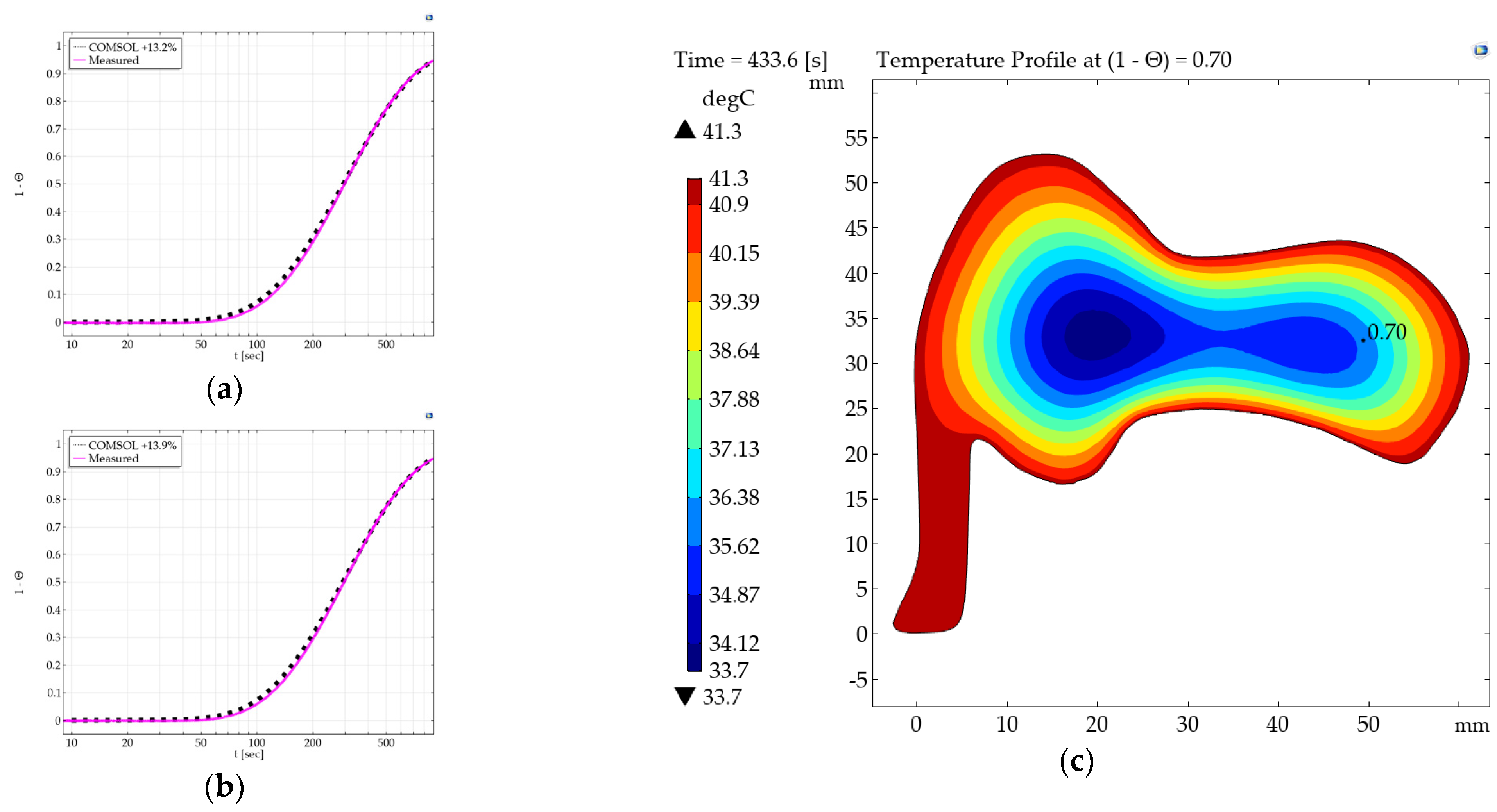
3.3. Comparison of Experimental Elephant and COMSOL

A hole was drilled from one side of the elephant to a prescribed internal position as with the spheres (Figure 6b). The thermocouple was place at this position and temperature was recorded over time and compared with the numerical simulation, as symmetry could no longer be applied. Figure 10 below shows two measurements and deviations from 3D simulations with the point of measurement marked with a black dot.

4. Discussion

4.1. Validation of COMSOL Simulation and Theory

To no surprise, the validation of the COMSOL model using the analytical theory for a sphere proved a success. As shown in Figure 11, the COMSOL model tracked the analytical solution with virtually no deviation at the comparison point of (1 − Θ) = 0.70 or 34 °C.

4.2. Comparison of Experimental Sphere Measurements, Theory, and COMSOL

The accuracy of measurements varied with the position within the sphere. The center (r = 0 mm) measurements proved to be the worst performers. Figure 9 shows relatively large deviations from the theory and model and is an expected result. The center of an object with spherical symmetry is equally affected in space and time by imperfect placing of its tip. The asymmetric nature of the fluid flow, measurement equipment, and the hole drilled into a sphere disrupt the boundary condition of a uniform heat transfer rate at the surface. Thus, the measurements render a poor comparison with model results as the model did not incorporate any asymmetric features.

For the off-center positions (r = 14.8, 19.3 mm), the results were in good agreement with the model. These two measurement positions were located closer to the direction of fluid flow. The surfaces that influenced these measurement points exhibit much more consistent surface characteristics and flow regimes, and thus more consistent heat transfer rates. While the results in measurement point r = 19.3 mm were more accurate, it was located only 10.3 mm away from the nearest surface. This excluded a major portion of the material from the measurement. A meaningful bulk material property measurement is representative of the largest possible proportion of the sample tested. Therefore, the best measurement recorded during this study was r = 14.8 mm.

4.3. Comparison of Experimental Elephant Measurements COMSOL

The deviation of measurements from the ideal boundary condition $\mathrm{Bi}=\infty$ for the elephant was between the measurements made at the center of spheres (r = 0 mm) and r = 14.8 mm. The deviation from model output indicates effects indicative of an inconsistent boundary condition. The position measured experienced thermal effects from surfaces that did not conform well with the assumption of a constant heat transfer rate at the surface. Figure 12 below shows a widthwise-vertically oriented slice along the axis of the drilled hole. The point of measurement is indicated with a white dot.

It is apparent that the region of the lower belly is close enough to influence the point of measurement. This area experiences a very different flow regime from the surfaces that meet the flow first. In addition, the legs are sinks to heat augmenting the temperature evolution with surfaces outside the assumption of constant heat transfer.

5. Conclusions

The results of this study have found a viable method of determining thermal diffusivity via a transient temperature measurement inside an object immersed in a moving fluid and comparison with a numerical simulation. The use of 3D-printed material was particularly challenging as the objects created did not exhibit consistent quality. Nevertheless, simulated temperature profiles in COMSOL were congruent in shape to the measurements in tests using spheres and the elephant. The next logical step would be to take the related theory and results to support the construction of a test rig capable of measuring a cylindrical geometry.

The method developed here can now be used as follows with an example of a cylindrical bore probe. The bore probe will be packed in foil to prevent drying, and a temperature sensor (or two) will be placed close to the center with known positions. The cylinder shall be stable in temperature (e.g., ambient) and will be placed in a water bath or oven with different and constant temperature. The recorded temperature versus time will be compared to numerical simulations of the same geometry and by fitting the thermal diffusivity, matching measurement, and simulation, the effective property is obtained. In case thermal conductivity is required, the specific heat capacity of the sample and density must be measured with other standard analytic instruments like calorimetry.

Establishing the necessary boundary conditions for assumed $\mathrm{Bi}=\infty$ is critical. Flow conditions need to be determined with a robust margin to guarantee that $\mathrm{Bi}\ge 120$ is achieved and difference between $\mathrm{Bi}=120$ and $\mathrm{Bi}=\infty$ is negligible. Further, a larger object may require either a larger fluid bath or larger fluid stream as the Nusselt number scales with increasing characteristic length.

References

- National Academies of Sciences, Engineering, and Medicine. Manual on Subsurface Investigations; The National Academies Press: Washington, DC, USA, 2019. [Google Scholar] [CrossRef]
- Bovesecchi, G.; Coppa, P. Basic Problems in Thermal-Conductivity Measurements of Soils. Int. J. Thermophys. 2013, 34, 1962–1974. [Google Scholar] [CrossRef]
- Palacios, A.; Cong, L.; Navarro, M.; Ding, Y.; Barreneche, C. Thermal conductivity measurement techniques for characterizing thermal energy storage materials—A review. Renew. Sustain. Energy Rev. 2019, 108, 32–52. [Google Scholar] [CrossRef]
- Jannot, Y.; Degiovanni, A. Thermal Properties Measurement of Materials; John Wiley & Sons, Inc.: Hoboken, NJ, USA, 2018. [Google Scholar] [CrossRef]
- Maglic, K.D.; Cezairliyan, A.; Peletsky, V.E. Compendium of Thermophysical Property Measurement Methods Vol. 1, Survey of Measurement Techniques; Plenum Press: New York, NY, USA, 1984. [Google Scholar] [CrossRef]
- Maglic, K.D.; Cezairliyan, A.; Peletsky, V.E. Compendium of Thermophysical Property Measurement Methods Vol. 2, Rec Mmended Measurement Techniques and Practices; Springer USA: Boston, MA, USA, 1992. [Google Scholar] [CrossRef]
- Zhao, D.; Qian, X.; Gu, X.; Jajja, S.; Yang, R. Measurement Techniques for Thermal Conductivity and Interfacial Thermal Conductance of Bulk and Thin Film Materials. J. Electron. Packag. 2016, 138, 040802. [Google Scholar] [CrossRef] [Green Version]
- Czichos, H.; Saito, T. Springer Handbook of Materials Measurement Methods; Smith, L., Ed.; Springer: Berlin/Heidelberg, Germany, 2006. [Google Scholar] [CrossRef]
- Czichos, H.; Saito, T. Springer Handbook of Metrology and Testing; Smith, L., Ed.; Springer: Berlin/Heidelberg, Germany, 2011. [Google Scholar] [CrossRef]
- VDI. VDI Heat Atlas, 2nd ed.; Springer GmbH: Berlin/Heidelberg, Germany, 2010; ISBN 978-3-540-77876-9. [Google Scholar]
- Hetnarski, R.B. Encyclopedia of Thermal Stresses, 2014th ed.; Springer: Berlin/Heidelberg, Germany, 2013; pp. 6186–6198. [Google Scholar]
- COMSOL Multiphysics® v. 5.5. Stockholm, Sweden. Available online: www.comsol.com (accessed on 20 July 2021).