1. Introduction
Global energy-related CO
2 emissions surpassed 30 Gt in 2010 and were above this benchmark throughout the whole decade, reaching 33.4 Gt in 2019, with some slowdown during the pandemic (31.5 Gt in 2020 [
1]). With globally recognised urgency for decarbonisation of the global economy, the success of bending the global emission curve downwards depends on the steps taken in every country and every economic sector, but especially in the electricity sector. The electricity sector alone comprises around a third of total CO
2 emissions (12.3 GtCO
2 in 2020 [
2]). However, decarbonisation of electricity generation opens a roadmap for decarbonisation of transportation, industry, and end-use sectors through electrification [
3,
4].
Primarily depending on fossil fuels for its energy requirements, India is already the third-largest emitter of CO
2, with 2.3 Gt from energy in 2019 [
5], though further growth in energy consumption is required to meet development goals. Having limited domestic fossil energy options, India currently imports roughly 90% of the crude oil and half the natural gas consumed in the country, with a quota of coal [
5,
6]. Further growth in energy consumption may increase India’s dependence on coal and energy imports. While growth in imports undermines national energy security and increases vulnerability to global markets, further growth in fossil fuel combustion may also raise air quality concerns.
Historically, the primary source of energy in Indian electricity generation has been coal. Thermal generation (coal, gas, oil) in total contributed around 60% to the generation mix [
7]. The total installed capacity more than doubled in the past decade, from 143.8 GW in 2009–2010 to 370.1 GW in 2019–2020 [
8], while the structure of production notably changed towards non-fossil energy sources: traditional nuclear and hydro, as well as recently progressing solar and wind energy. India has shown remarkable progress in integrating intermittent renewables with the electric power grid, reaching >20% of total generation capacity and >8% in total generation.
Progress in renewable energy is achieved by both policy and dramatic reduction in the costs of photovoltaics and wind turbines, making them highly cost-effective [
9]. After joining the Paris Accord [
10], India introduced various policies pledging to reduce intensity of its gross domestic product by 33–35% from 2005 levels by 2030, with 40% of its cumulative installed capacity from renewable energy sources [
11]. The government also set a renewable energy target of 175 GW of capacity by 2022 (100 GW solar, 60 GW wind power, 10 GW bioenergy, and 5 GW small hydro) and 450 GW by 2030 [
12]. The steps taken in the implementation of these goals have already brought notable results, and if this continues, India may achieve the INDC (intended nationally determined contributions) goals even earlier or exceed them by 2030 [
5]. Still, the country’s power sector CO
2 emissions are approaching 1 Gt (960 MtCO
2 in 2019–2020 vs 520 MtCO
2 in 2007–2008). India continues to build coal-fired power plants to secure its energy needs.
India’s high potential for renewable energy along with cost reductions could be a possible answer to further energy growth without jeopardising the transition to economic prosperity and sustainability. Thanks to its geographic location and 250–300 sunny days a year, India has solar energy irradiation of an average of 4–7 kWh/m² per day throughout the country [
13]. Covering 3% area of waste land by solar photovoltaics modules can add around 750 gigawatts [
14], which will generate roughly the annual total consumption of 2019. Wind energy has also significant potential in southern and eastern parts of the country, with varying estimates of up to 3400 GW [
15]. However, even if the annual potential of solar and wind energy far exceeds reasonable needs, the intermittent nature of these energy sources creates challenges for grid integration along with creating redundant generating capacity, which in turn leads to lower capacity utilisation of the electricity system (see, for example, [
16]). With the growing penetration of renewable energy sources into the electricity system, the inherent challenges of intermittent supply, uncertainty, variability, and reliability become major issues [
17,
18].
The hourly match of supply and demand is harder to achieve when electricity supply is defined by geophysical and meteorological conditions and demand is defined by consumer needs, which is beyond the control of the system operators. Balancing technologies, such as energy storage, backup or fixed firm capacity, and manageable demand, becomes increasingly important in the high-renewable power grid. However, the need for balancing can potentially be reduced in the planning stage of the power system itself. Different generation profiles and repetitive patterns of wind and solar resources across locations could be taken into account. Selecting locations with long-term wind–solar and spatial complementary patterns and proper sizing of capacities across locations along with the power grid may minimise variability in the total electricity supply.
The complementarity of intermittent energy sources can be defined as a negative correlation of long-term hourly generation time series. As such, even if generation patterns do not precisely repeat themselves in terms of days, seasons, and years, there might be a strong correlation of output from technologies in neighbouring or distant locations. A negative correlation between intermittent energy sources is especially valuable in building a diversified generation portfolio that reduces balancing needs.
To take advantage of this potential complementarity between resources, long-term power system planning is indispensable. Considering more locations with different generation profiles and more extended time series will lead to more robust results. This necessitates using large-scale modelling to take into account long-term data and optimise spatial allocations of electricity-generating capacities towards building a resilient, robust, cost-efficient, carbon-free power system.
A growing number of studies are addressing the challenges of building power systems with a high share of intermittent renewables, evaluating potential obstacles and limits, properties, and requirements of full-renewable systems. In general, a growing share of intermittent renewables may reduce systemwide electricity costs, and 100% renewable systems have been shown technically feasible and economically viable for number of countries and regions, including India.
TERI [
19] has undertaken a techno-economic assessment of expansion of renewables in 2025–2030. Applying the open-source modelling framework PyPSA [
20] to the power sector in India, the study estimates the share of variable renewable energy sources to reach 26% in the baseline and 32% in high-renewable scenarios (or 42% and 47%, respectively, if hydro, biomass, and nuclear are included) without raising the total economic costs. Higher penetration of renewables requires further study.
Lu et al. (2020) developed cost minimisation model to evaluate India’s potential for integrating solar and wind energy by 2040 using reanalysis weather data from NASA (MERRA-2 and GEOS-5 datasets). Authors concluded that India could satisfy 80% of the expected demand in 2040 with wind and solar energy, and lower costs. Still, coal plays a significant role as a backup capacity, balancing the power system throughout a year [
21].
Gulagi et al. (2017) explored 100% renewable energy transition pathways for India until 2050 using a set of alternative energy storage, generation, and few demand-side technologies to balance demand and supply. The authors found that energy storage plays a growing role in the system, but levelised systemwide costs of electricity can be potentially lower than the current level [
22]. The technical feasibility of 100% renewable energy for India is also concluded by Lawrenz et al. (2018), who considered heat and transportation sectors along with electric power, and further discussed potential social, economic, and political barriers of the energy transformation [
23].
Geospatial complementarity of solar and wind energy with transmission can play a balancing role and mitigate seasonal variation in production, such as the monsoon effect [
24,
25]. The connection of distant regions with high-voltage power grids can provide additional balancing options, improve reliability, and reduce costs of multi-country power systems [
22].
Another important source of balancing high-renewable energy systems is demand-side flexibility. It can be modelled by sector coupling, when demand-side technologies are explicitly considered, or based on assumptions regarding the potential demand shift in time or reduction. Balasubramanian and Balachandra develop a mixed-integer linear-programming model to study demand-side interventions as potential solutions to managing the challenges associated with renewable energy integration and found the interventions to be effective in moderating variability associated with electricity demand [
26]. Lugovoy et al. (2021) considered different types of demand-side technologies with different properties and requirements, showing their role in storage reduction in a 100% renewable scenarios for China [
27].
The discussed studies apply different models and software to access the operation and expansion of the power sector with a high share of renewables, though all of them share similarities in methodology. This included linear cost-minimisation modelling framework to optimise capacity structure of the power sector, and one-hour resolution to represent intermittent energy sources and energy storage. Moreover, the discussed models have several regions connected with electricity transmission lines; the production of renewables is defined by capacity factors, estimated based on weather data in modelled regions. Such a framework represents the state of the art in long-term energy system modelling. However, analyses with a high share of renewables can also benefit from higher spatial resolution to better represent intermittency and complementarity across locations. Consideration of alternative weather years can also improve the robustness of the results for long-term planning.
The earlier studies of 100% renewable systems for India, discussed above, have reached hourly representation with a full year of weather data (8760 h) for up to 10 regions. However, the chosen weather year and the number of locations of renewables are not always clarified. In this study, we further explored a potential transition of the Indian electric power system to carbon neutrality around mid-century using large-scale modelling with improved granularity and number of weather years. Scenarios in the study are optimised for 41 years of hourly weather data, 32 regions connected with the transmission grid, 114 spatial locations (clusters) of wind, and 60 of solar energy.
We intentionally limited energy supply sources to wind and solar to evaluate the structure and features of such a 100% renewable power system, the potential for complementarity of the energy sources across locations, and the role of alternative balancing options including demand-side flexibility. We used the larger scale data and designed a set of 153 scenarios to study the concept of a wind- and solar-based power system for India with balancing requirements. Forty-one years of hourly weather data capture long-term complementarity patterns across locations and the two energy sources. Instead of proposing particular storage technologies with different duration profiles, we use one generic storage and study intraday and longer duration in each scenario to evaluate intermittency patterns, complementarity effects, and substitution between different balancing options. Additional technologies, such as hydro and biomass energy, can be considered in further studies to evaluate their role and impact on the required balancing options and costs.
This paper is organised as follows.
Section 2 presents the data and methods and assumptions used in the IDEEA model, i.e., a power system optimisation model with potential for extension to whole energy sector optimisation.
Section 3 presents the results and discussion, including capacity and generation profiles, seasonality and storage duration, interregional trade and demand flexibility, system-wide levelled costs for multiple scenarios, and transition dynamics.
Section 4 presents a summary and conclusions.
2. Data and Methods
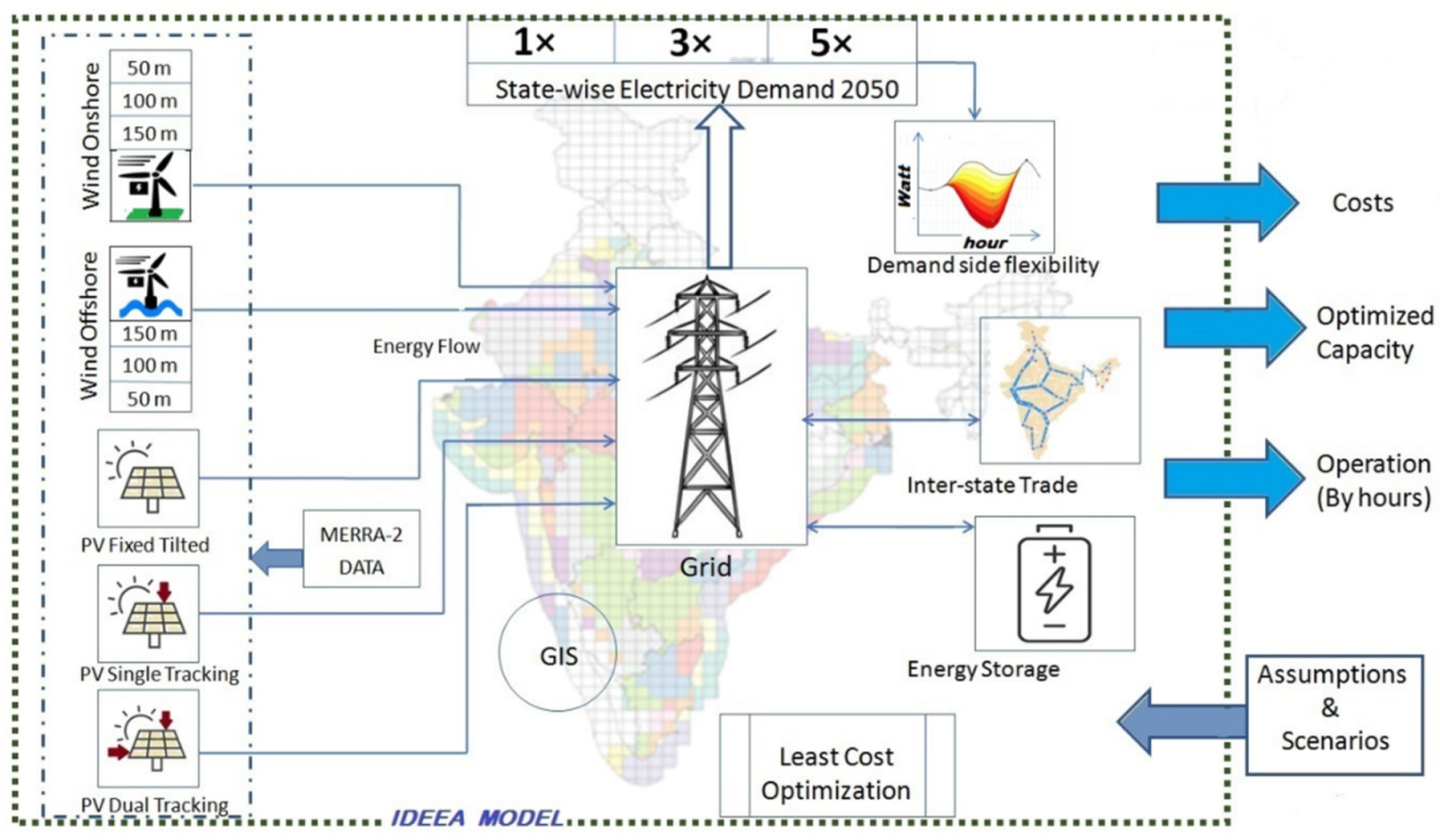
This section discusses the data and methodology used in achieving a zero-carbon pathway by 2050 for India. Geographic information system (GIS) data and 41 years of Modern-Era Retrospective Analysis for Research and Applications (MERRA)-2 data were used to estimate solar and wind potential across the country in achieving this objective. India’s installed capacity and technology-based generation profile for FY 2019–2020 were used to validate the model developed.
2.1. IDEEA Model
The IDEEA model adopts a capacity-expansion framework for electric power systems, with potential extension to whole energy system optimisation. Formerly known as reference energy system or bottom-up energy system models—and recently, macro-energy systems [
28]—this modelling approach combines engineering with economics. Energy and materials (commodities) are measured in physical quantities. Commodities can be produced, transformed, stored, and transported with various technological processes (technologies). Every process has a set of simplified but close-to-reality characteristics (parameters), such as efficiency and costs. Technologies can be combined into technological chains to convert the primary supply and resources (e.g., coal, gas, oil, biomass, solar, wind, hydro-energy) into usable energy (electricity) or any other commodity specified as the final demand.
The technological chains compete in the model based on their potential, availability, and cost. The least expensive option that satisfies all the resource requirements and additional constraints (such as policies) is considered optimal for each scenario. However, multiple scenarios are generally required to address uncertainty in the data, technological parameters, or costs to study the sensitivity of the modelling results to different sets of assumptions. Well-known examples of macro-energy models and model generators with a focus on whole energy systems are TIMES/MARKAL [
29], MESSAGE [
30], TEMOA [
31], OSeMOSYS [
32], and ReEDS [
33]. Examples of power system models are Switch [
34,
35], PyPSA [
20], and GenX [
36]. The family of models is growing rapidly; more can be found on the Open Energy Modelling Initiative website [
37].
The current version of the IDEEA model is based on the energyRt [
38], an open-source model generator implemented in R [
39]. This package has sets of classes and methods to generate an energy system model, create a dataset for the model formulated in an algebraic programming language, solve the model, read the solution, and process the results for comparative analyses. It has an embedded generic energy system model translated into several algebraic programming software languages (GAMS, Python/Pyomo, Julia/JuMP, and GLPK/MathProg). Around 100 predefined constraints (the model equations can be found on the software website) are activated, depending on the configuration of the model. Basic energy models developed with energyRt have been compared to other software, and deliver identical results after harmonisation of parameters [
40].
The IDEEA model is also integrated with the Indian GIS information for quick linkage with geospatial datasets (such as MERRA-2), evaluation of available land, and distances between interregional power grid nodes. The number of regions in the model is scalable. A 34-region version is presented in
Figure A1 and
Table A1, though for the current study we focus on 32 mainland regions. Every region in the model can be split into territorial clusters to address spatial variations in wind and solar patterns within the region. A total of 114 spatial clusters for wind energy and 60 for solar energy are considered in this paper.
Time resolution in the IDEEA model is also flexible. All scenarios in the study, except ‘transitional’, have 1-hour steps for 8760 total hours per year. Having every hour of a year represented in the model is essential for modelling the intermittent nature of renewable systems and proper sizing of balancing options. A schematic representation of the IDEEA model structure used to study a 100% renewables power system design is shown in
Figure 1.
2.2. Wind and Solar Energy Potential
Due to its proximity to the equator, India has sturdy solar energy potential with low variation throughout the year. The resource is substantial in all regions, though it varies based on elevation, humidity, and precipitation. Several regions in India also have substantial wind resources. Recent studies have identified renewable energy sources in India as 850–3400 GW for onshore wind and 1300–5200 GW for utility-scale photovoltaic power, based on geospatial analysis and economics [
15]. These estimates were based on technological assumptions, land availability, and costs.
Continuous advancement in technologies and reductions in cost render systems more productive and accessible. For example, current mainstream photovoltaic technologies have 15–21% efficiency [
41], meaning that only around 20% of solar radiation exposed on a photovoltaic panel can be transformed into electricity. According to the National Renewable Energy Laboratory, the best laboratory practices exceed 40% efficiency [
42]. This growth in efficiency means reduction in land used, the same area being able to accommodate twice the capacity if efficiency doubles. The efficiency of wind turbines tends to grow as well. Every technological upgrade, such as a higher hub for wind energy, efficiency improvement of photovoltaics, extends the technical boundaries of their application, and lowers costs to make these technologies economically more attractive.
We use MERRA-2 data [
43] to evaluate the long-term potential of solar and wind resources and hourly electricity output for several types of wind and solar power generation technologies. The reanalysis data are a product of Earth system models that use satellite images to reproduce historical geophysical processes, including wind speed, solar radiation, and precipitation. MERRA-2 [
44] and ERA5 [
45] datasets are open to the public. Though such reanalysis data may have a potential bias for some locations if compared with direct observations [
46,
47], still the data are quite close to reality and available for literally every location in the world for every hour of more than four decades, making this a good source of information for high-renewable systems.
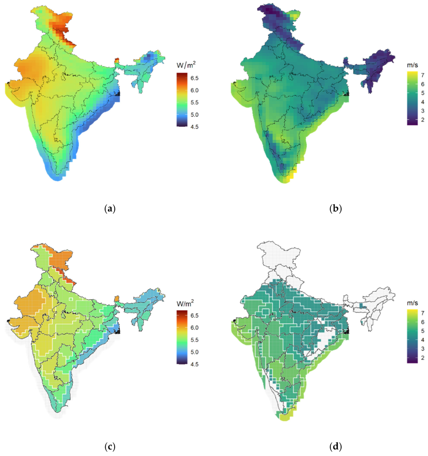
Figure 2 shows 41-year averages (1980–2020) of global horizontal irradiance (incoming shortwave flux on a horizontal surface) and wind speed at 50 m height for every cell of the MERRA-2 grid (roughly 50 × 60 km for India’s latitude). The total number of spatial-grid cells is 1200 with offshore territories. Every cell of the grid can be considered a long-term hourly time series (starting 1 January 1980 at 12:00 a.m. and ending 31 December 2020 at 11:00 p.m.) with around 360,000 observations (hours). The solar radiation data have been used to evaluate electricity generation by solar photovoltaics with three types of trackers (fixed tilted installation with an optimal angle equal to the latitude, one-axis tilted tracker, and dual tracker).
The average height of modern turbines is >70 m, with some being >200 m. Such heights are not available in the MERRA-2 dataset. Therefore, we extrapolated wind speed at higher altitudes using a dynamically estimated wind gradient: the Hellmann constant based on the given wind speed at 10 and 50 m for every hour. The authors realise that such extrapolation adds to the uncertainty in the wind speed measurements and may introduce additional potential bias. Therefore, we designed scenarios with and without wind speed extrapolation to study the sensitivity of the results to these methodological assumptions.
The potential hourly output for every technology is represented as an hourly capacity factor for every spatial grid cell using the merra2ools package for R [
48]. The package reproduces Sandia’s plane-of-array model and algorithms for solar-array trackers [
49]. In addition, it uses an average of wind power curves of several mainstream wind turbine models.
The clusters were defined using 41 years of hourly correlations between neighbour cells separately for solar radiation and wind speed. Additional clustering criteria were geopotential height (from MERRA-2) and estimated long-term average capacity factors. The number of clusters for every IDEEA region represents at least 85% of the variation of the considered indicators.
Figure 2c,d show the resulting 114 spatial clusters for wind and 60 for solar energy. Locations with lower than 20% average annual availability were dropped. Offshore wind locations were associated with the closest region based on the proximity of every cell to the mainland regions.
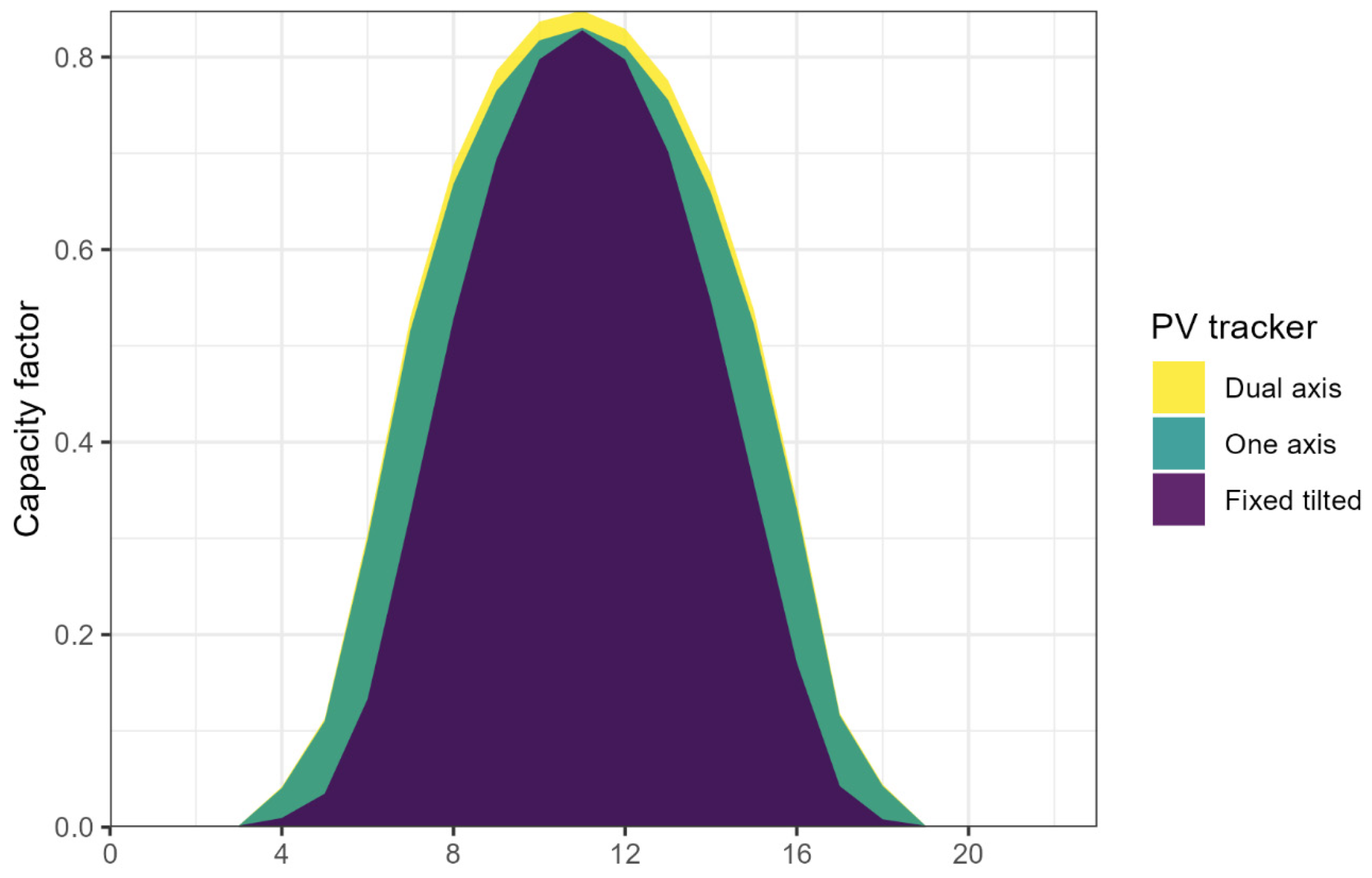
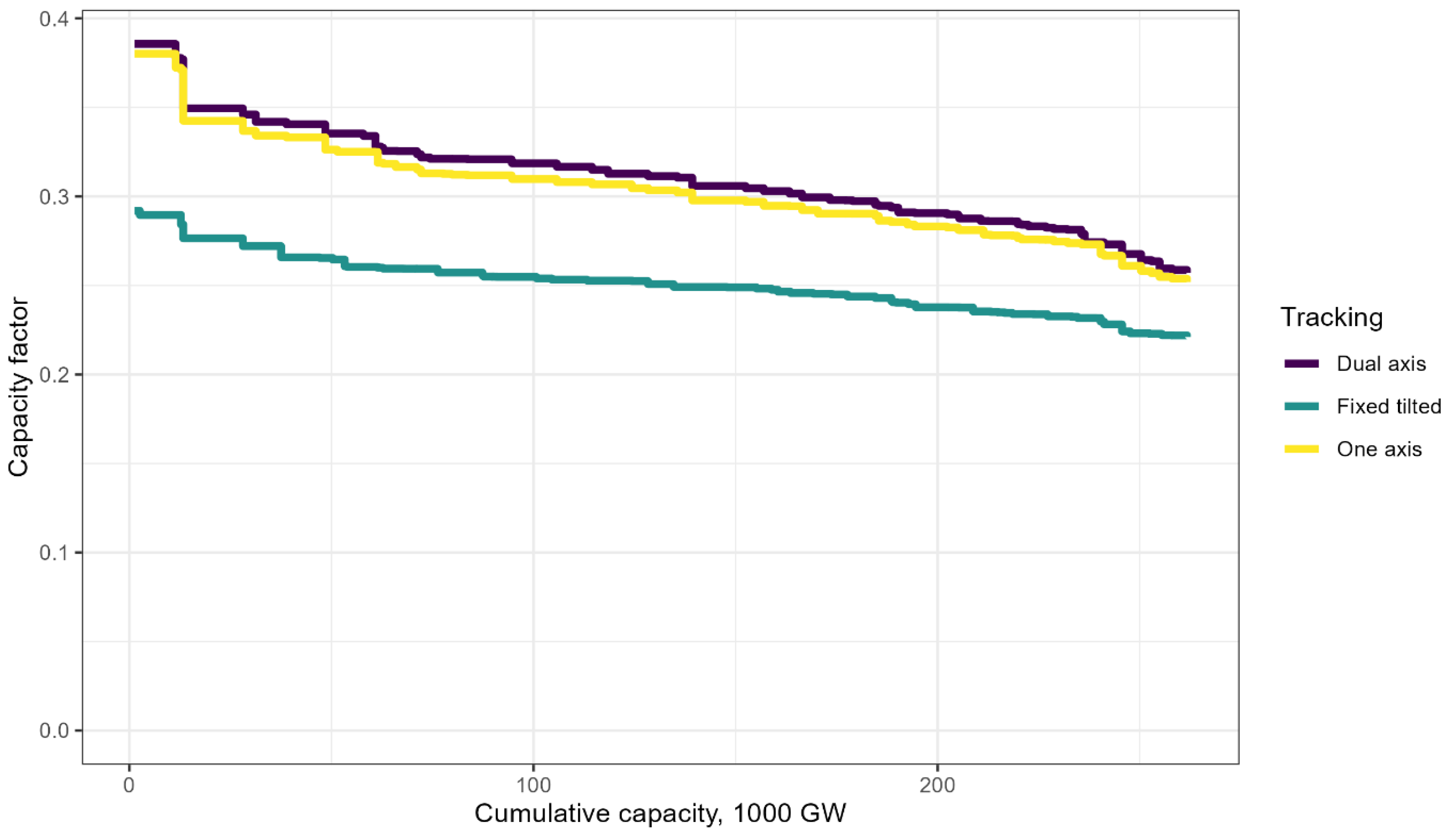
Figure A2 in
Appendix A compares the long-term average performance of three types of photovoltaic trackers used in this study. The main gain in generation happens when moving from fixed models to one-axis tilted tracking. This type of tracking captures more sun during the day by tilting the panel to the east in the morning and tracking its progress towards the west during the day. While the second axis tracker adds some value during peak hours, the overall gain in production is not so significant. Still, this type of tracking offers the highest generation throughout a year.
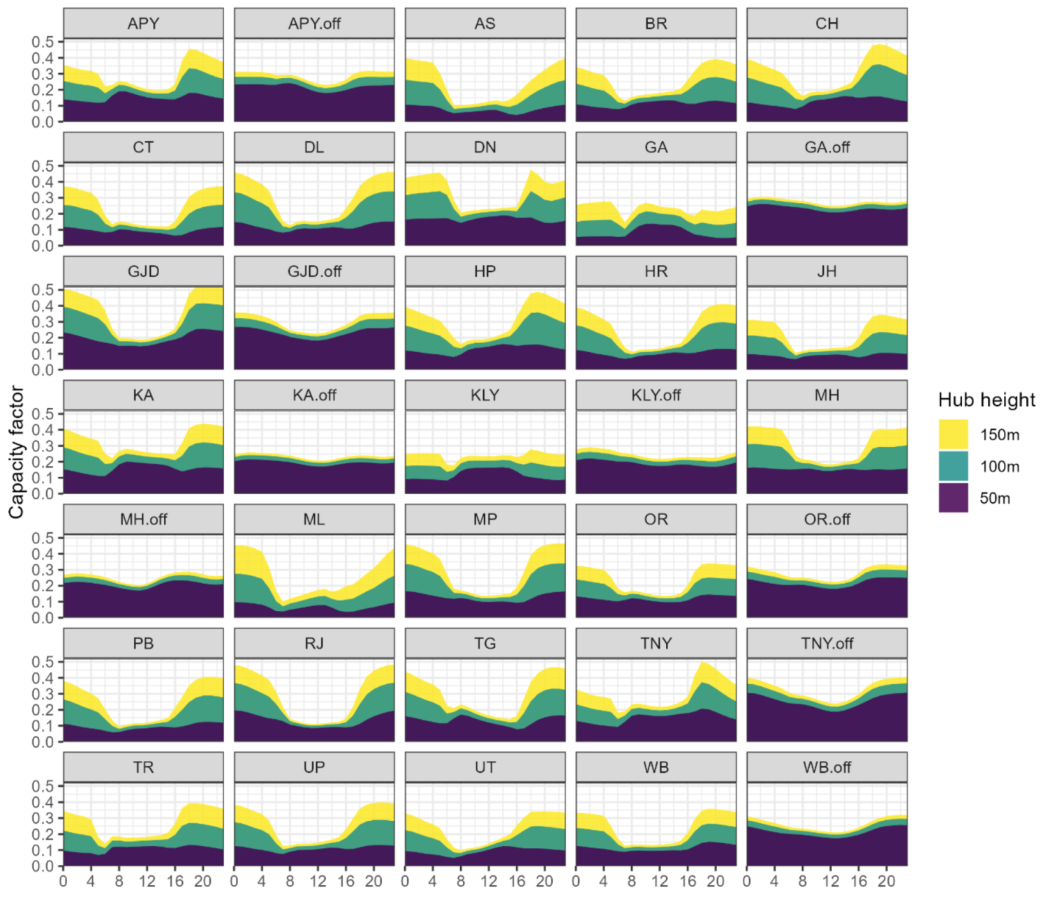
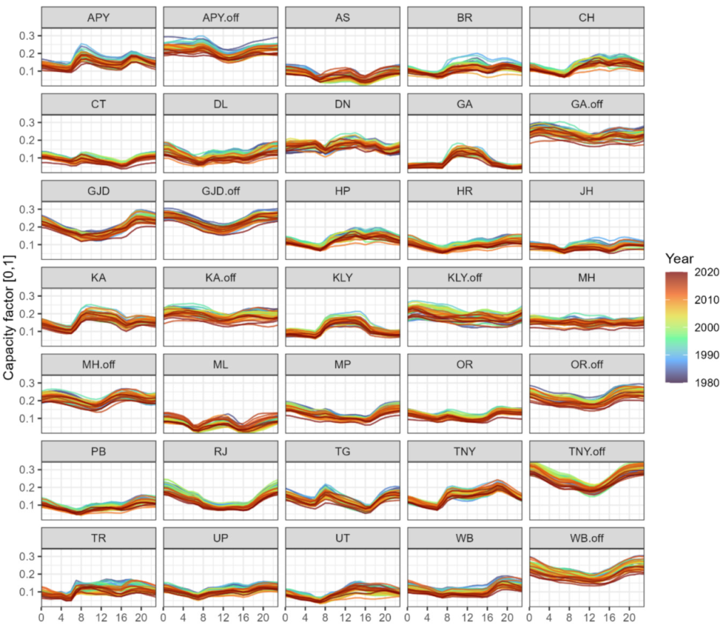
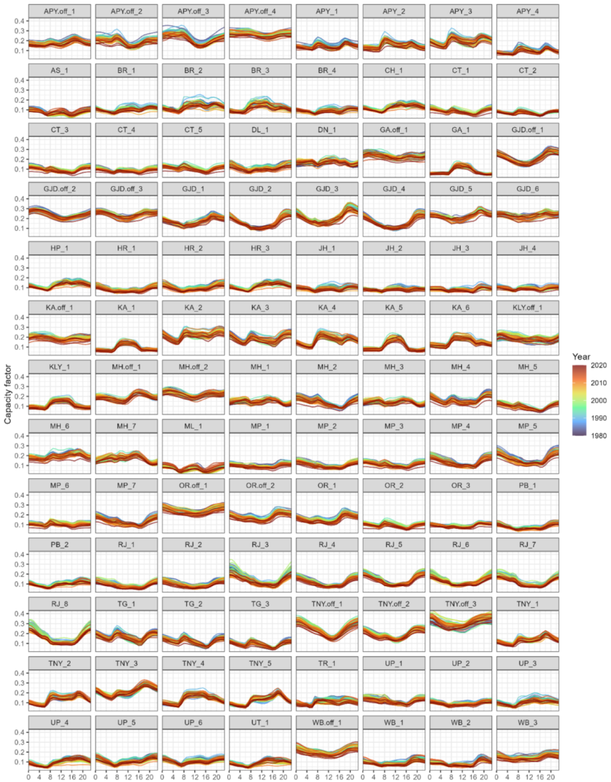
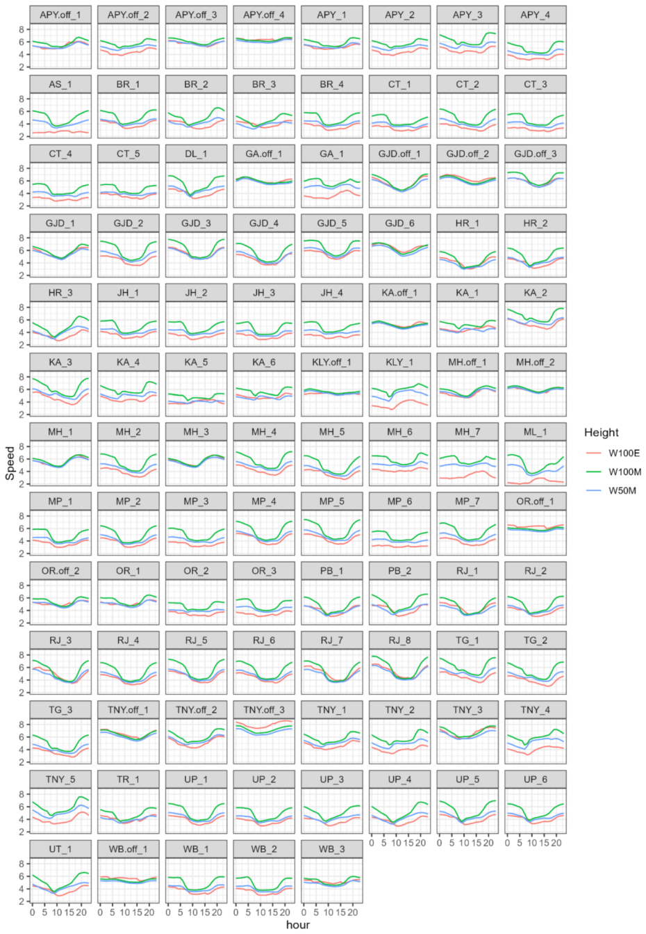
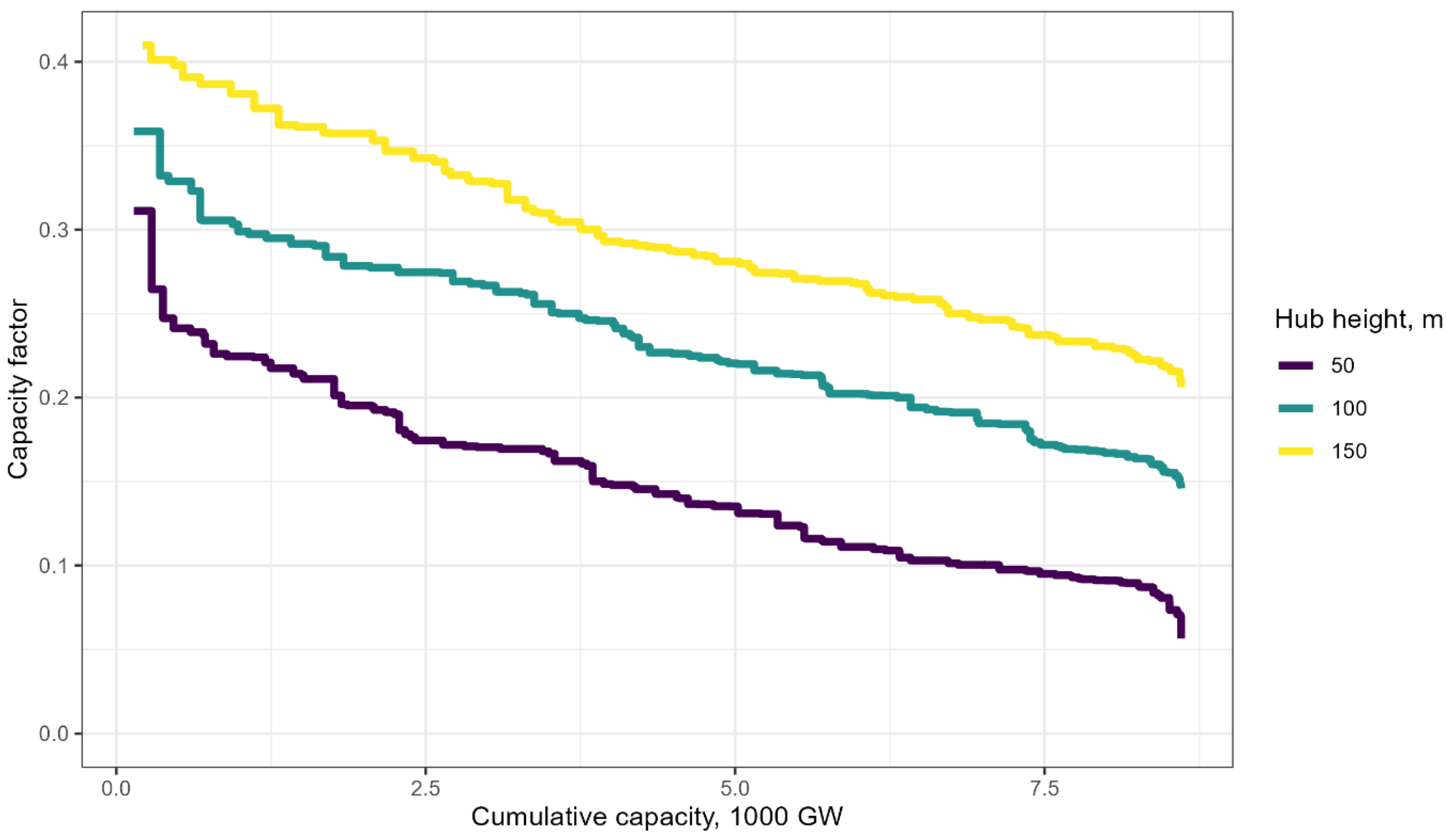
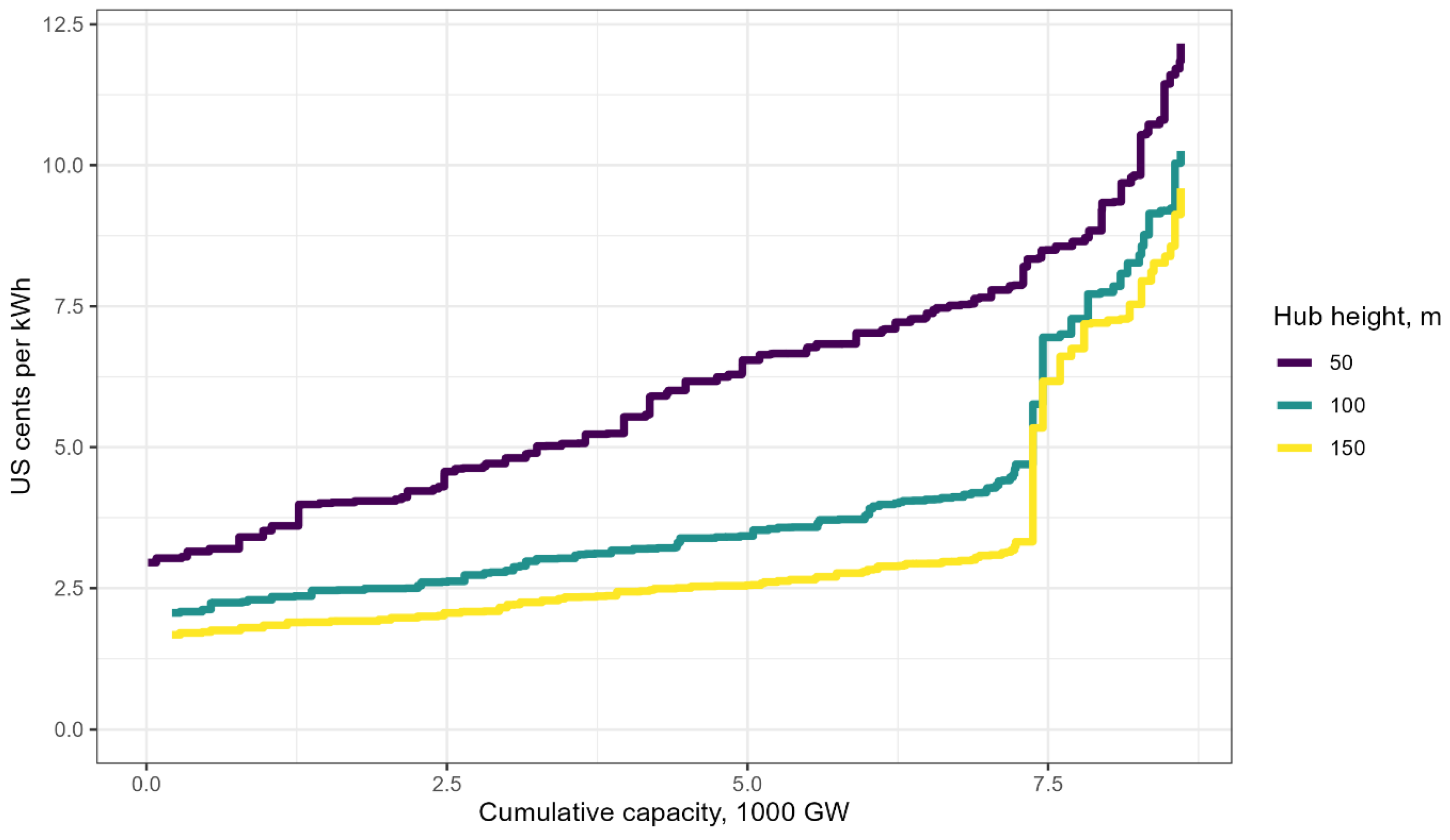
Figure A3 shows the estimated average intraday performance of wind turbines for 50, 100, and 150 m hub heights. The difference in production is driven by the wind speed. The estimated 100 and 150 m capacity factors show higher levels of production and also higher variation in wind speed during a day. The slowdown of wind in the daytime and increase in night hours have been observed in India before [
50,
51]. It is also visible on 50 m data from MERRA-2 and consistent through all 41 years (see
Figure A4 and
Figure A5 for average diurnal capacity by year). Such intraday profiles are opposite to solar energy and thus highly complementary.
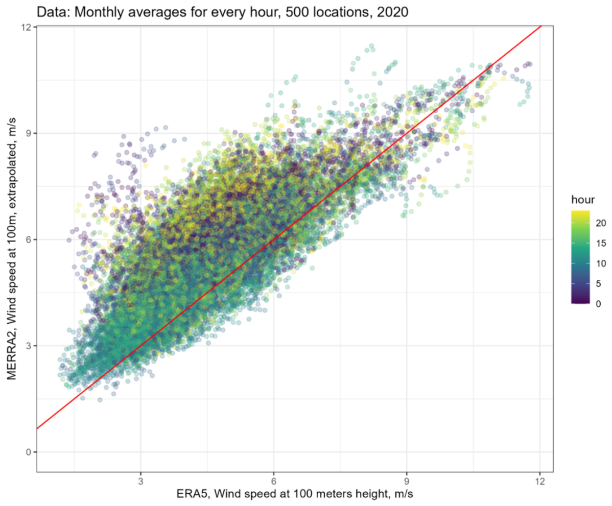
This diurnal wind speed variation in MERRA-2 was also observed in the ERA5 reanalysis database (see
Figure A6), which reports wind speeds at 100 m height, though the ERA5 data show overall less wind for India than MERRA-2 and extrapolated data show higher variations in wind speed (see also
Figure A7). The increase in wind speed differences between day and night hours is a result of a negative correlation of wind speed at 10 and 50 m height in MERRA-2 data. The direct extrapolation might have a bias and should be validated by real measurements. If confirmed, the higher hubs might also be more beneficial, due to higher complementarity with solar energy.
2.3. Technological Assumptions
Wind speed and solar radiation for every MERRA-2 grid cell and every hour of the past 41 years were further used to evaluate capacity factors for alternative wind power plants and photovoltaic system-tracking technologies. (Capacity factors were defined as a coefficient of 0–1 that represents capacity utilisation, a share of current electricity production from its nameplate peak for every location of potential installation and every hour. Capacity factors within an hour were equal for all installations within the same territorial cluster.) We considered three options for wind turbines: 50, 100, and 150 m hub height. The power curve and costs per megawatt of capacity, required land use, and the power curve linking wind speed with power generation were assumed to be the same for the three technologies. Therefore, the difference between wind power output of the technologies is driven by wind -speed differences at different heights and offshore wind installations also have higher costs. Similarly, we considered three types of solar trackers for photovoltaic systems: fixed tilted, one-axis tilted tracker, and dual tracker.
The goal of considering different solar and wind power technologies is a sensitivity analysis of results to different technologies and assumptions. There was only one type of wind generator and one solar power plant present in every particular scenario. Wind technologies did not compete based on performance and costs, and different solar technologies were not compared within one scenario. All types of solar or wind power generation technology were assumed to have the same costs and not vary across regions.
Hourly capacity factors predetermine the supply of electricity in every location. With known hourly generation potential, the total electricity supply can be optimised by sizing the generation capacity in every location, subject to given demand and the available balancing options. When wind and solar energy are the only source of electricity, both have exogenous supply predetermined by model input. Matching demand and supply can be achieved by balancing technologies, such as storage and grid. Energy storage offers intertemporal balancing by accumulating energy when it is bountiful and discharging when the generation is lower than the load demanded. On the contrary, the electric power grid can be used for spatial balancing between connected areas, dispatching electricity from regions with high generation to locations with a deficit.
Several storage technologies (batteries, hydro storage, compressed air, flying wheels) can be selected for a particular application based on the required duration of storage and costs. Similarly, long-distance grids offer different technologies (direct or alternate currents, voltage), resulting in varying levels of transmission losses, sizing, and costs. The goal of this study was instead to advise on the potential role of storage and the grid in balancing. Therefore, we considered generic energy storage with 80% roundtrip efficiency and generic power grid technology with 3% loss per 1000 km.
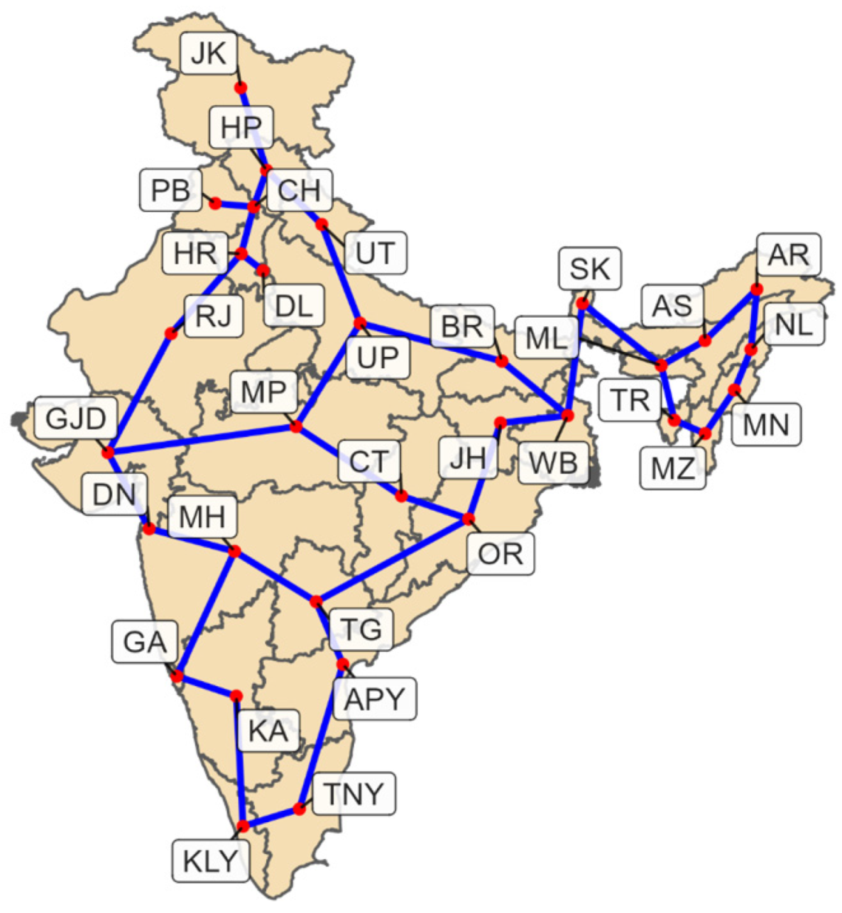
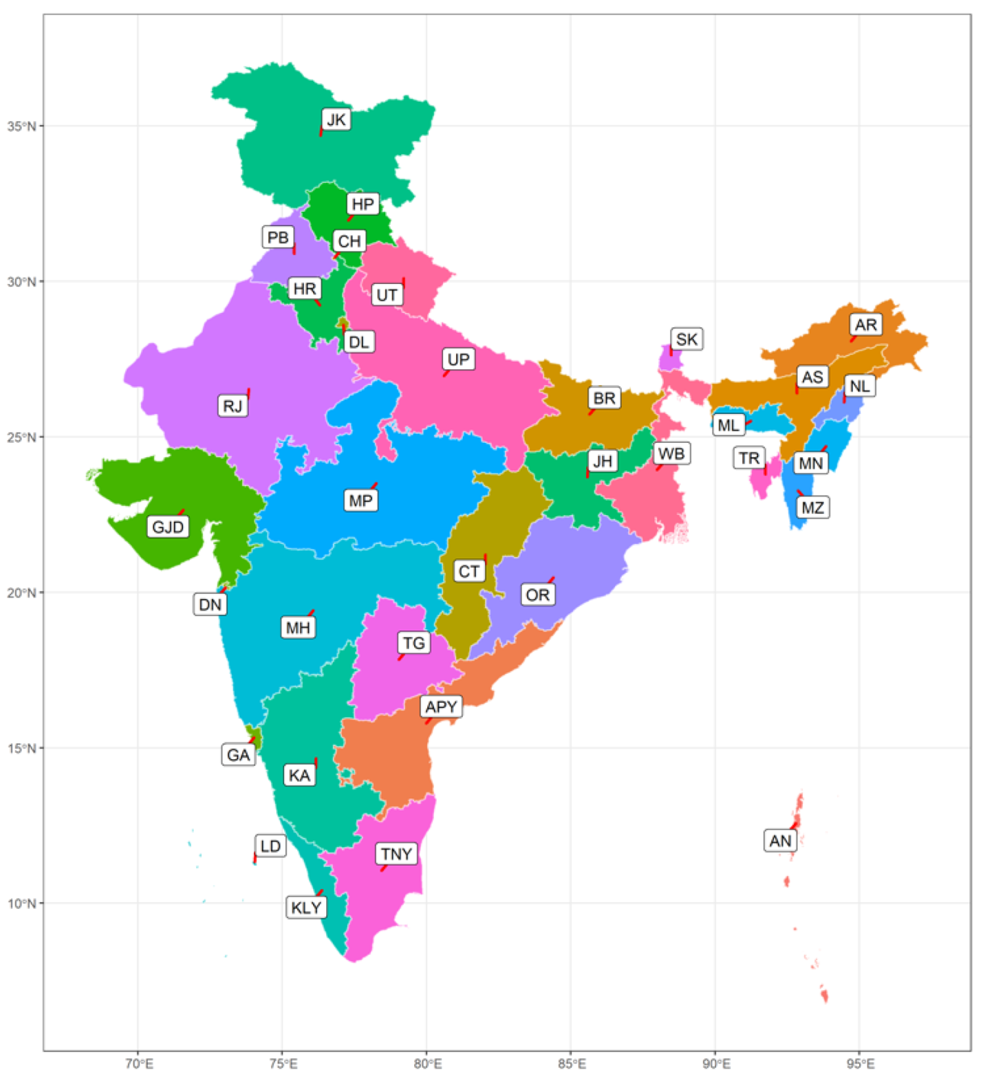
For simplicity and computational tractability of the scenarios with power grid technology, we limited the number of connections (nodes) on the nationwide transmission system to the number of regions (
Figure 3). The location of each node is the geographical centre of the region. The number of connections for every region is limited to three, ensuring that every region is connected to the network. Each of the 36 power lines is a different technology in the model. The length of every power line was defined as the horizontal spatial length between two nodes plus 15% for potential landscape variation.
Costs of solar and onshore wind technologies were taken from generic tariff orders issued by the Karnataka Electricity Regulatory Commission to determine tariffs for solar and wind power, which reflect market prices of domestically produced technologies for 2019 [
52,
53]. Offshore wind technologies are in the early development stage in India [
54]. We assumed that the cost of offshore installations was triple that of onshore, based on average international differences for the technologies [
55,
56]. Costs of energy storage and long-distance power grids were taken from international sources. Costs of every power line were also indexed for regions with differences in average elevation >1000 km and for regions with varying heights within the region.
Table 1 summarises capital cost assumptions for each technology.
We assumed that up to 10% of every territory could be used for wind turbine installations (assuming 6 MW/km
2) and up to 1% of the area in every solar cluster for photovoltaic installations (assuming 20 MW/km
2). In this paper, we do not locate where the installations will happen in every spatial cluster. Instead, we assume that the defined share of every cluster is suitable for the installations, using the land directly or combining with other economic activities, such as agriculture for wind turbines and buildings or highways for photovoltaics. The resulting nationwide cumulative supply curves for wind and solar energy are shown in
Appendix A,
Figure A8,
Figure A9,
Figure A10 and
Figure A11.
Another balancing option considered in the study was demand-side flexibility. Energy storage and power grids can be used to adjust electricity supply based on given demand. However, different demand-side technologies have different requirements: some can be adjusted to follow the supply. Demand-side management programs and time-of-use tariffs are designed to shift demand in time to improve efficiency and decrease overall system costs. Electrification, automation, and robotisation trends will probably increase the flexibility of demand-side technologies, making the intraday load curve more manageable. Optimisation of the supply-side and load curve can provide valuable insight into how much supply-side balancing options can be substituted by responsive demand.
Different demand-side technologies have different flexibility requirements. In this study, we considered technologies with the intraday shift. Potentially, these can encompass a broad group of end-use electricity consumers, including electric cars and trucks, air conditioning, water heating, refrigeration, charging of autonomous devices, cloud computing, and more. The assumed daily requirement for this technology group was fixed.
Finally, to track system inefficiency and achieve model convergence for all scenarios, we set a limit on marginal electricity costs of USD 1 per kWh. Suppose the system cannot deliver electricity in a particular hour and region. In that case, it will be ‘imported’ from ‘outside’ the modelled power system and considered unmet demand (‘unserved’ in figures) or system failure to deliver electricity. On the other hand, generated but unconsumed electricity is regarded as curtailed supply (‘curtailed’ in figures).
2.4. Scenarios
The set of scenarios in this paper was designed to study the potential and intermittent nature of solar and wind energy sources separately and together to evaluate the role of alternative balancing options and address uncertainty regarding technological parameters and the final demand. With this goal, we considered four dimensions (branches) of scenarios with three to five sets (groups) of alternative parameters in each branch, as summarised in
Table 2.
The first branch of scenarios comprises alternative combinations of supply-side technologies, starting from one energy source (solar or onshore wind), continuing with combinations, and finally adding offshore wind. Scenarios with only one energy source are helpful for understanding that source’s pure potential, intermittent nature, and requirements for balancing options to serve demand. Further combination of several generation sources highlights potential complementarity and benefits of mixing different energy sources in terms of reducing required energy storage and power grid.
The second branch comprises five alternative balancing options. The ‘none’ group of scenarios does not have any technology to balance supply with demand, other than sizing the supply and overbuilding generation capacity. The model optimises generation capacity (solar photovoltaic panels and wind turbines) in each region to minimise costs of supply, unmet demand, and curtailment. This group also helps to evaluate the pure complementarity of wind and solar energy on long-term historical weather data. Another two balancing options are energy storage and interregional electric power grid. Adding generic energy storage identifies hours where there is a lack of supply and evaluates how much energy should be moved in time to serve the load within each region.
On the contrary, the electric power grid can be used to balance supply and demand spatially every hour. In scenarios where the technology is available, the model sizes all the considered interregional power lines. The combination of storage and power grid adds both spatial and temporal balancing options to the model. The last balancing option in the branch is the flexibility of the demand side. This group of scenarios has the option to partially manage the load curve within a day.
The last two branches in the scenario matrix address uncertainties in the data and future demand for electricity by setting a range of possibilities for technological parameters (‘technological optimism’) and the level of final demand. The ‘level of demand’ branch addresses uncertainty regarding the potential level of electricity consumption in 2050 and beyond. We introduce three demand scenarios: actual level of 2019 (1×), triple (3×), and fivefold (5×) the demand of 2019.
The role of the ‘technological optimism’ branch of scenarios is studying the effects of technological uncertainty on the results. As discussed in the Data and Methods Section, wind speed data at 50 m from MERRA-2 must be extrapolated to obtain numbers on heights for modern wind power turbines that capture stronger winds. Any chosen extrapolation procedure adds to the uncertainty and can potentially introduce systematic or unsystematic bias. This extrapolation error can be addressed by validation and bias-correction procedures if real measurement data are available. In this study, we did not have enough information to validate the extrapolated wind speed data. Instead, we considered scenarios based on un-extrapolated data (50 m) and data extrapolated for 100 m and 150 m, analysing differences in results and leaving validation for further research.
The four branches of scenarios give 180 possible combinations (4 × 5 × 3 × 3), where 144 scenarios have fixed (‘FLAT’) load assumptions for every hour within a year. The remaining 36 scenarios have an endogenous demand structure with the ability to optimise daily load by shifting it within 24 h. The model optimises the share of the responsive demand and the shape of the hourly load curve of the responsive part of demand in all the 32 regions and every day.
Figure 4 compares structures and levels of total annual demand by scenarios. The ‘FLAT’ type indicates fixed time load, constant every hour of a year for every region. At least 25% of total demand in every region is reserved for ‘FLAT’ load. The remaining 75% is the area for optimisation, a choice between ‘FLAT’ and ‘FLEX-24h’ load type in every region, based on price signals, to be discussed.
Two-level electricity pricing is another assumption in scenarios with responsive demand. Fixed flat load requires guaranteed electricity supply for 24 h, 365 days a year. In contrast, the responsive load requires a certain number of watthours within a day, where hours of dispatch and consumption are negotiated between electricity producers and consumers. Indeed, the two types of electricity supply (‘FLAT’ and ‘FLEX-24h’) are different market products with different characteristics and should be priced differently. Since the rigid ‘FLAT’ demand is harder to deliver with intermittent renewables, this type of supply requires more balancing, potentially has more curtailments, and is thus more expensive. As such, for every kilowatt hour of electricity supplied to the ‘FLAT’ load, we set a credit to work as an external subsidy in the model and serve as a price signal for the production side that adjusts generation capacity and balancing technologies to reach the minimal system costs with the introduced price credit. The flexible part of demand was also priced with much lower credit to distinguish this part of demand from curtailments (losses).
Setting different credits will result in different shares of the two types of loads. In the paper, we set the price credit for the ‘FLAT’ load as the average of levelised costs of generation (without balancing) and total levelised system-wide electricity costs (with balancing) in scenarios with ‘FLAT’ demand. The credit for ‘FLEX-24 h’ was set to half the cost of generation in every region. This rule serves to demonstrate cost savings.
In total, we report comparative results for 153 scenarios: 144 with constant load and nine with partially flexible load. The responsive demand option is a substitute for daily energy storage. The role of the storage option is already reflected in the ‘stg’ and ‘stg+grid’ groups of scenarios. Therefore, we report the demand-side balancing option (+dsf) only for scenarios with all generating technologies to demonstrate the potential savings in storage by making part of the load responsive within 24 h. All 153 scenarios were solved based on 2020 weather data (MERRA-2). In addition, several scenarios were solved based on 41 years of weather data in one model run to test the long-term viability of the system (see
Table 3).
Solving the model with 8760 h of weather data and around 180 clusters (wind and solar combined) is computationally intensive. A scenario with 1 year’s weather data takes a few hours to solve with dual or primary simplex algorithms (CPLEX solver by IBM). An approximate solution can be achieved in 10–20 min with a barrier algorithm and 10−5 tolerance (equivalent to about 10 MW in the model) on a consumer-level PC with at least 16 Gb of RAM. The 41 years of weather scenarios have roughly 200,000 non-zero data points for each of 180 locations, expanding the initial LP matrix to roughly 500 million rows and columns and 1.5 billion non-zeros.
The 41-weather-year model was formulated to optimise all the capacity in the first year of optimisation but serve throughout the 41 weather years. Optimisation was performed in one step, equivalent to perfect foresight multiyear optimisation modelling. The discount factor was set to zero to equalise alternative weather years in the objective function. Investment costs with 5% capitalised interest payments were annualised and considered annual fixed costs in the model. The lifespan of all technologies was set to exceed the number of weather years. Such settings make the multi-weather-year optimisation equivalent to a 1-year optimisation, with the difference being that the optimisation results fit any of the 41 weather years considered equally (1980–2020). Limiting the investment variables of the model to the first year made the solution tractable. With a problem-reduction routine (performed by the solver), the dimension can be reduced to a matrix with 50–100 million rows and columns and 200–300 million non-zeros, depending on the scenario. Still, the 41-year scenarios require up to 500 Gb of RAM and 30–50 h to solve using a barrier algorithm on a 48-core workstation.
3. Results and Discussion
The scenarios developed outline potential solutions for wind and solar energy-based electric power systems in India, with alternative technological options and assumptions. Scenarios with only one energy source (wind or solar) or no/minimal balancing options are extreme cases that evaluate boundaries of the space of potential technically feasible options. Comparing such corner-solution cases with technological mixtures provides insights into the complementarity of technologies and the benefits of considering them together.
The comparative metrics include total generating and balancing capacity, hourly operation of the system, seasonality, and regional allocation. Although all 153 scenarios have the same 2020 weather year of input data, 11 have been additionally solved on 41 years of data to test the system’s long-term viability and the robustness of the solution for alternative weather years.
3.1. Capacity and Generation Profile
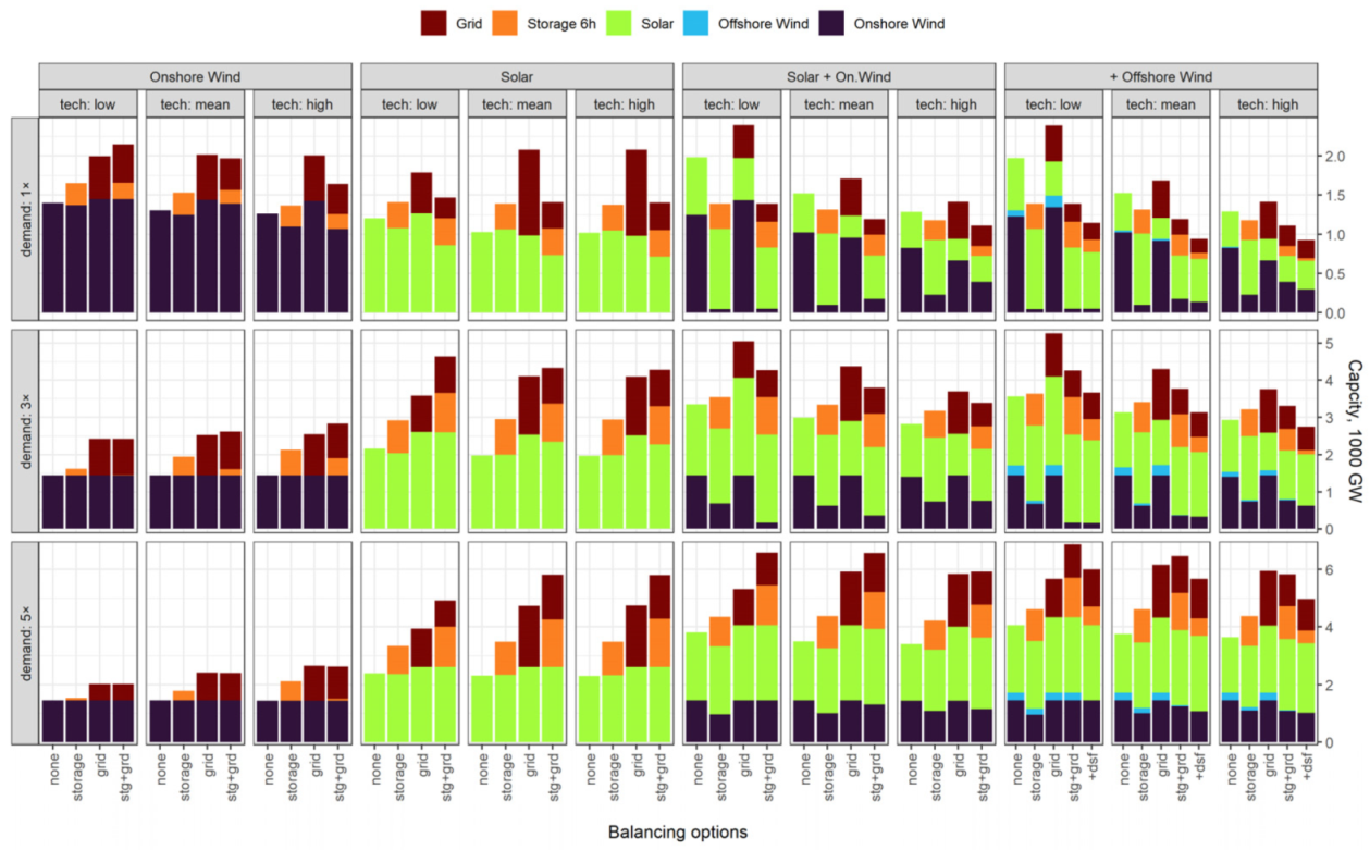
The structure of the generating and balancing capacity of the 153 scenarios is compared in
Figure 5 and generation profiles are shown in
Figure 6. The scenarios are grouped by branches. Each of the 36 cells in the figures has four or five scenarios with alternative balancing options (
x-axis) for the same level of technological optimism (‘tech’). Furthermore, the scenarios are grouped by generating technologies (top) and the level of demand. Every bar in
Figure 5 represents the installed capacity of onshore and offshore wind turbines, solar photovoltaic systems, 6-h storage, and aggregate grid capacity in thousands of gigawatts.
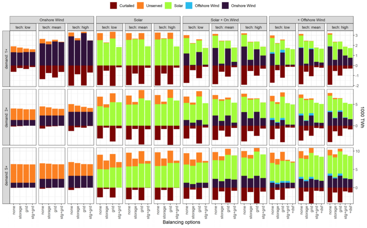
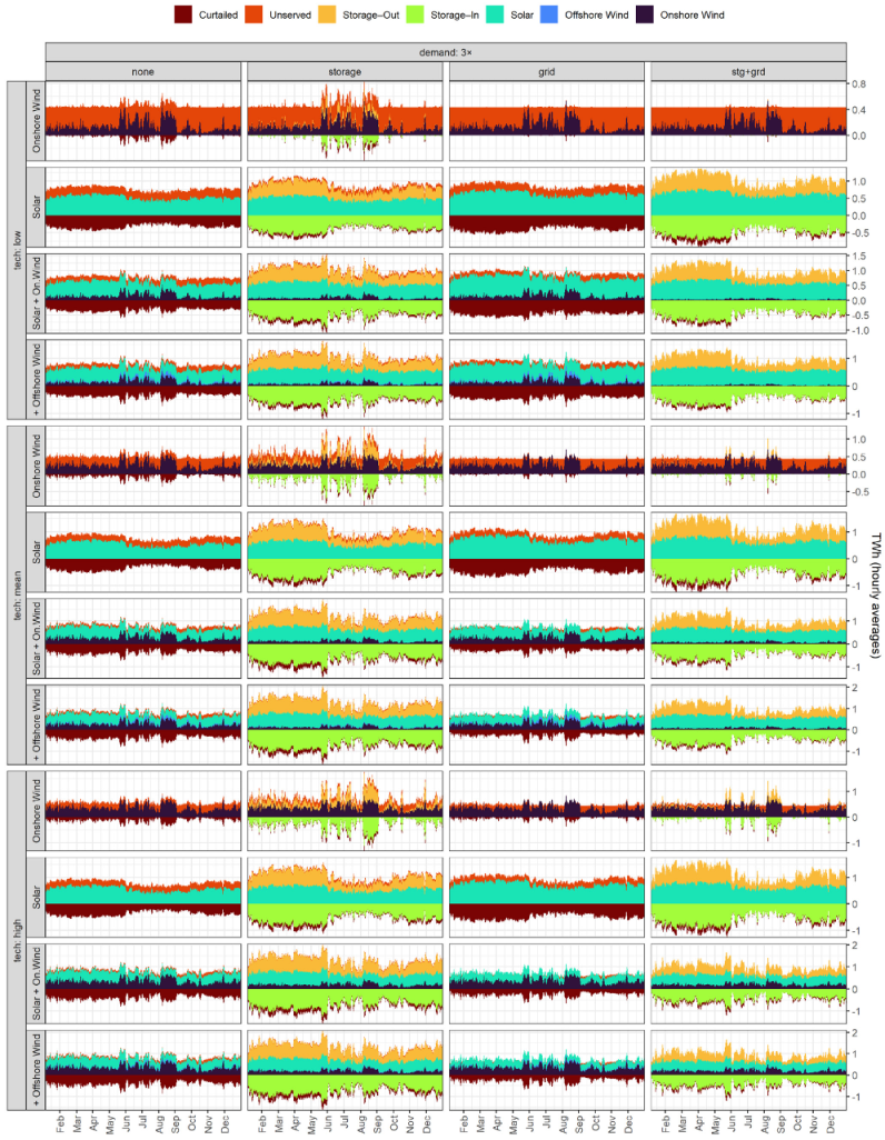
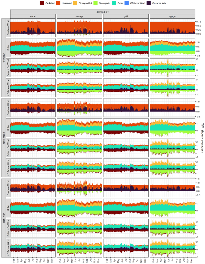
Figure 6 shows the generation structure by technology, unmet load, and curtailed generation.
The unmet load (‘Unserved’) in
Figure 6 indicates the system’s failure to deliver electricity. The height of the bar, when compared with the annual level of demand (1300 TWh in ‘1×’ scenarios; 3800 and 6400 TWh in ‘3×’ and ‘5×’ scenarios, respectively) gives an insight on the share of unmet demand. The curtailed energy supply demonstrates system inefficiency in serving a given demand. Higher curtailments indicate a mismatch between production and consumption by hours throughout the year: the system generates more electricity than consumed, but cannot achieve balance with the options available, other than overbuilding the generating stock. Scenarios with no or lowest unmet load, curtailed energy, and the low-levelised costs of energy might be considered for further evaluation and potential implementation.
Based on the results, wind or solar energy source and no balancing technologies (‘none’ on
x-axis) serve roughly 50% of annual demand (‘1×’ group). Balancing options (‘storage’, ‘grid’, ‘stg+grd’ on
x-axis) increase the served share of the demand up to 100%. Though wind resource is reaching its boundary quickly, less than 50% of annual load can be delivered in ‘3×’ and ‘5×’ demand scenarios with wind energy only. Solar generation reaches its specified 1% land area maximum potential in ‘5×’ scenarios, as indicated by curtailments in the ‘solar’ group with storage- and grid-balancing options (‘stg+grd’,
Figure 5).
Even when balancing technologies are not available, the combination of solar and wind energy reduces the system failure to meet the demand from roughly 50% to 10–25%, depending on demand and technological assumptions (compare ‘unserved’ bars in ‘solar + on. wind’ vs ‘solar’ and ‘onshore wind’ and ‘none’ groups for different ‘demand’ and ‘tech’ groups;
Figure 6).
Offshore wind is a more expensive option and appears only in ‘low optimism’ scenarios and higher-demand scenarios (3× and 5×) when the total wind resource is close to its limit (see ‘+ offshore wind’ scenarios).
The capacity of installed wind energy in wind-only scenarios is generally higher than in solar-only scenarios (see ‘1×’ demand level, ‘wind’ vs ‘solar’ groups). Higher technological optimism leads to lower overall capacity along with significantly higher generation, especially for wind energy. Scenarios with 100 m wind turbine hubs (‘tech: mean’) have double the generation of 50 m hubs (‘tech: low’), and scenarios with 150 m turbines (group ‘tech: high’) show a 30% increase in generation for the same capacity. Differences between solar photovoltaic-tracker types are noticeable in the transition from fixed tilted panels (‘tech: low’) to one-axis tilted tracking (‘tech: mean’), and less visible in further transition to dual-tracking systems (‘tech: high’). As discussed in the Data and Methods Section, the differences in the performance of alternative technologies are driven by estimated capacity factors (see also
Figure A2 and
Figure A3 in the
Appendix A).
Storage and ‘grid’ play different roles when combined with alternative energy sources. ‘Grid’ reduces system failures when combined with wind energy but does not improve solar-only scenarios much. In contrast, storage improves solar-only scenarios dramatically, but does not affect wind-only scenarios much. The same pattern is observed in ‘solar + on. wind’ scenarios. When only storage is available for balancing (‘storage’, x-axis), wind capacity is the lowest in the optimised mix. In grid-only scenarios (‘grid’), wind energy tends to dominate. Unmet load is much lower, but still significant in scenarios with solar and wind energy and only one balancing option.
The dual-balancing option (‘stg+grd’) makes solar-only scenarios technically feasible, with close to zero unmet load and minimal curtailments. Wind energy when considered individually can technically meet demand in ‘1×’ scenarios with 150 m hubs (‘tech: high’). Adding demand-side flexibility (‘+dsf’) to the balancing options reduces required storage several-fold and increases the share of solar across the three demand scenarios (1×, 3×, 5×).
Figure A12,
Figure A13,
Figure A14 and
Figure A15 in the
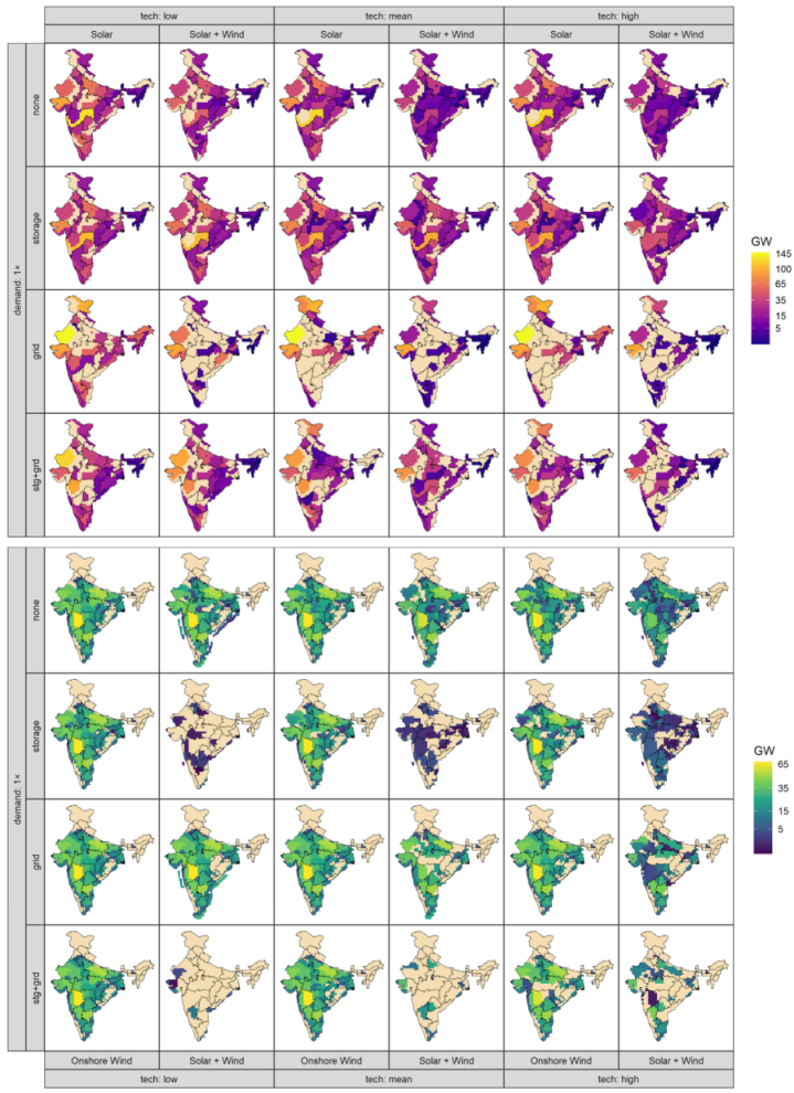
Appendix A show the optimised region-wise clustered generating capacity of solar and wind energy sources by scenario for demand levels of 1×, 3×, and 5×. For demand level 1× (
Figure A12) and solar-only scenarios with no balancing options, Maharashtra state has the highest capacity (around 145 GW in some clusters in the state). In comparison, the north-eastern states of Meghalaya and Mizoram have <5 GW worth of installed photovoltaic systems, driven by lower demand and lower potential of the energy source. With the storage-balancing option, the solar capacity in Maharashtra is still the highest, but lower (120 GW) than without balancing technologies. A further addition of the grid option changes the cost-optimal spatial allocation. The model now installs more solar photovoltaic systems in Rajasthan and Gujarat. Gujarat and Punjab have the highest solar + wind generation (around 35–40 GW), while north-eastern states (Manipur, Meghalaya, and Mizoram) have the minimum generation of <5 GW.
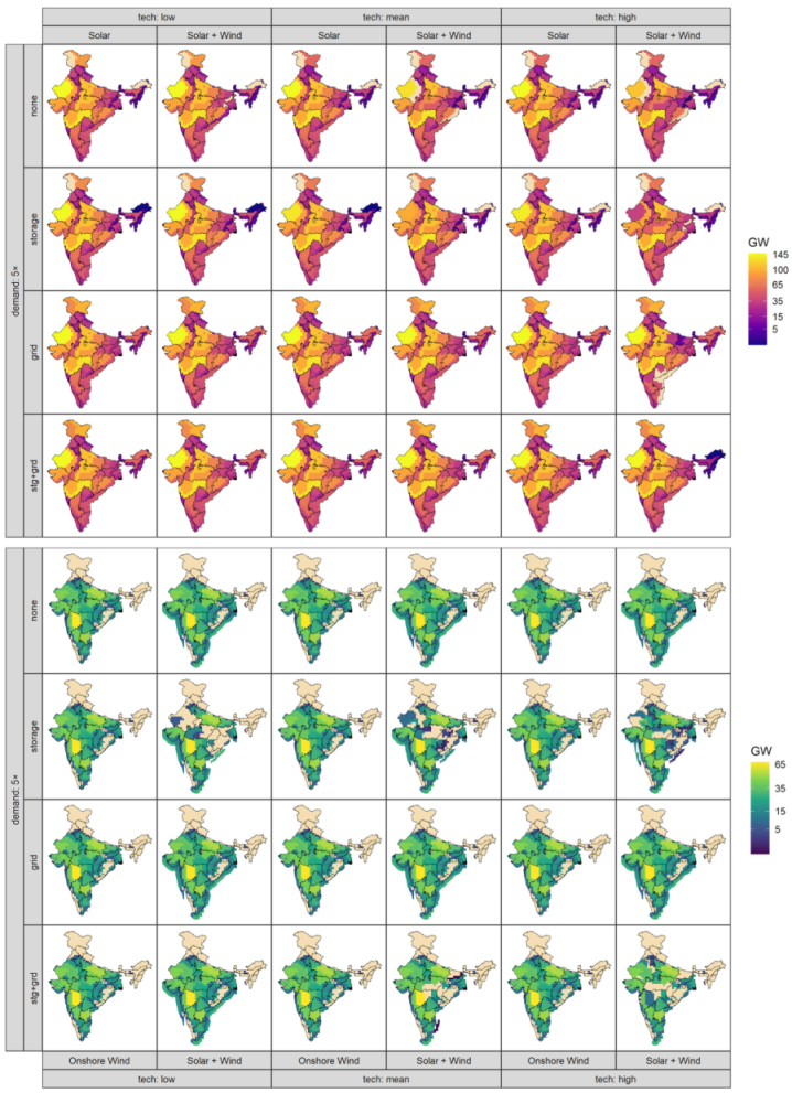
Higher ‘technological optimism’ and higher demand increase the overall role of wind energy, pushing installed capacity to its limits. Offshore wind plays more of a role in scenarios where onshore wind energy reaches its limits. Though the capacity utilisation of offshore wind is, on average, higher than onshore, the increase in cost is too significant, and this energy source is considered the last option (see also
Figure 2).
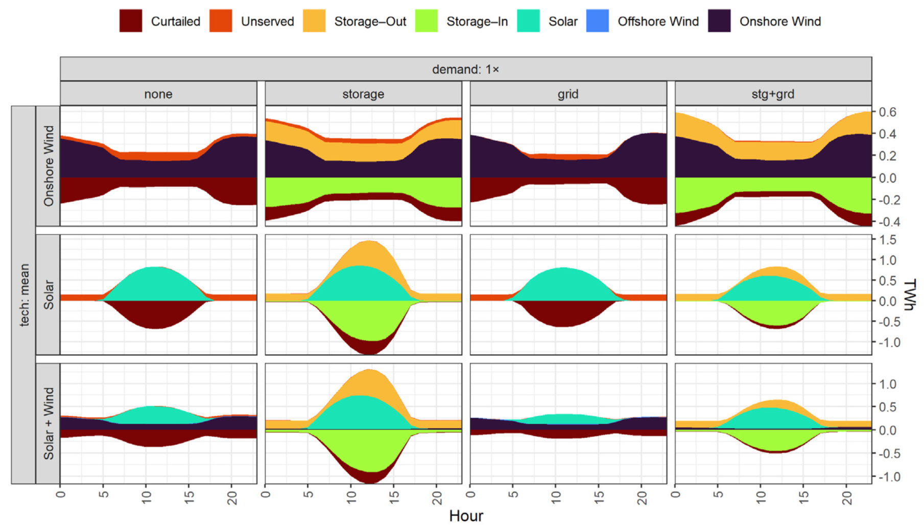
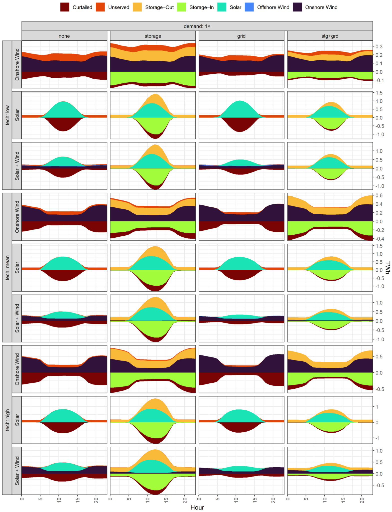
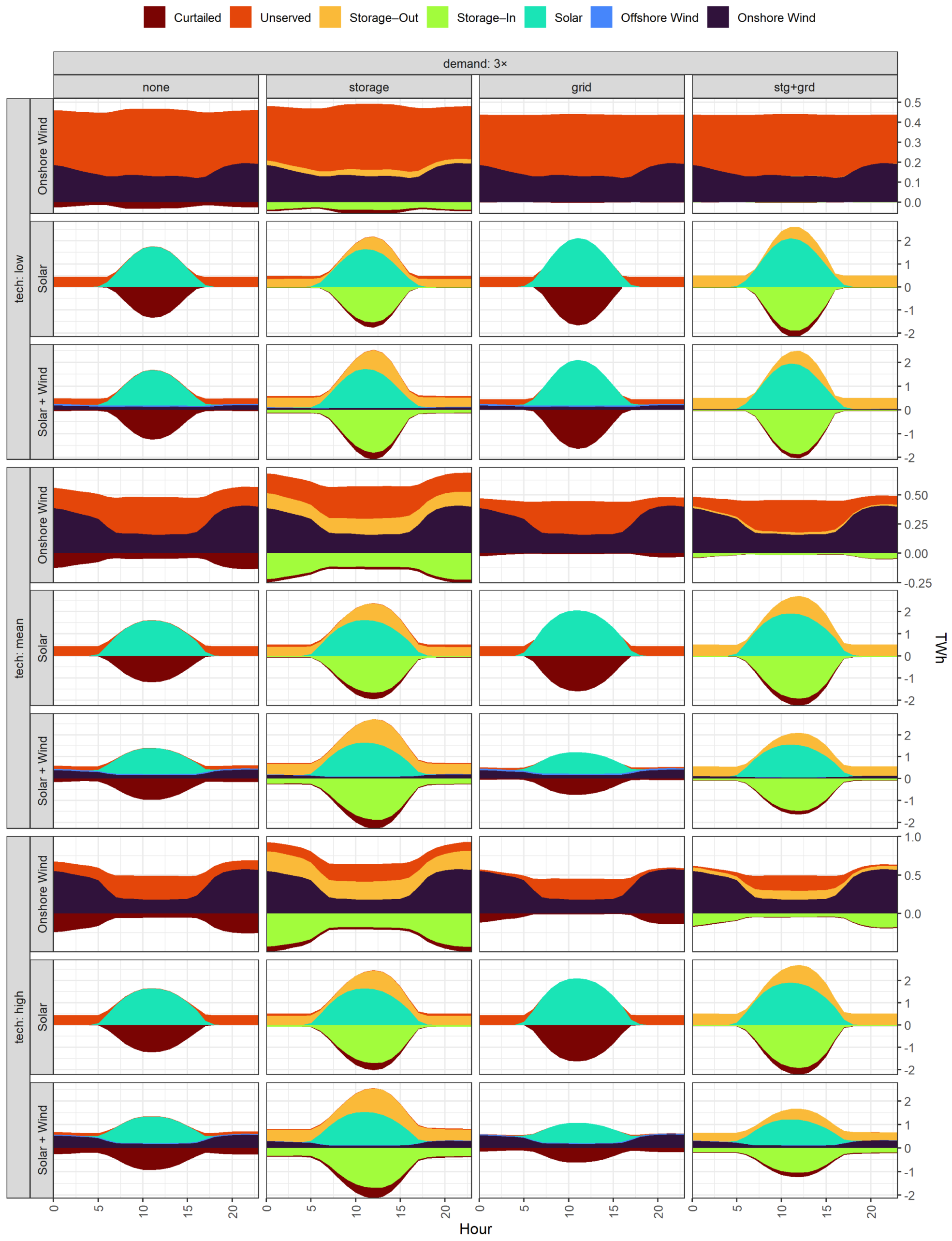
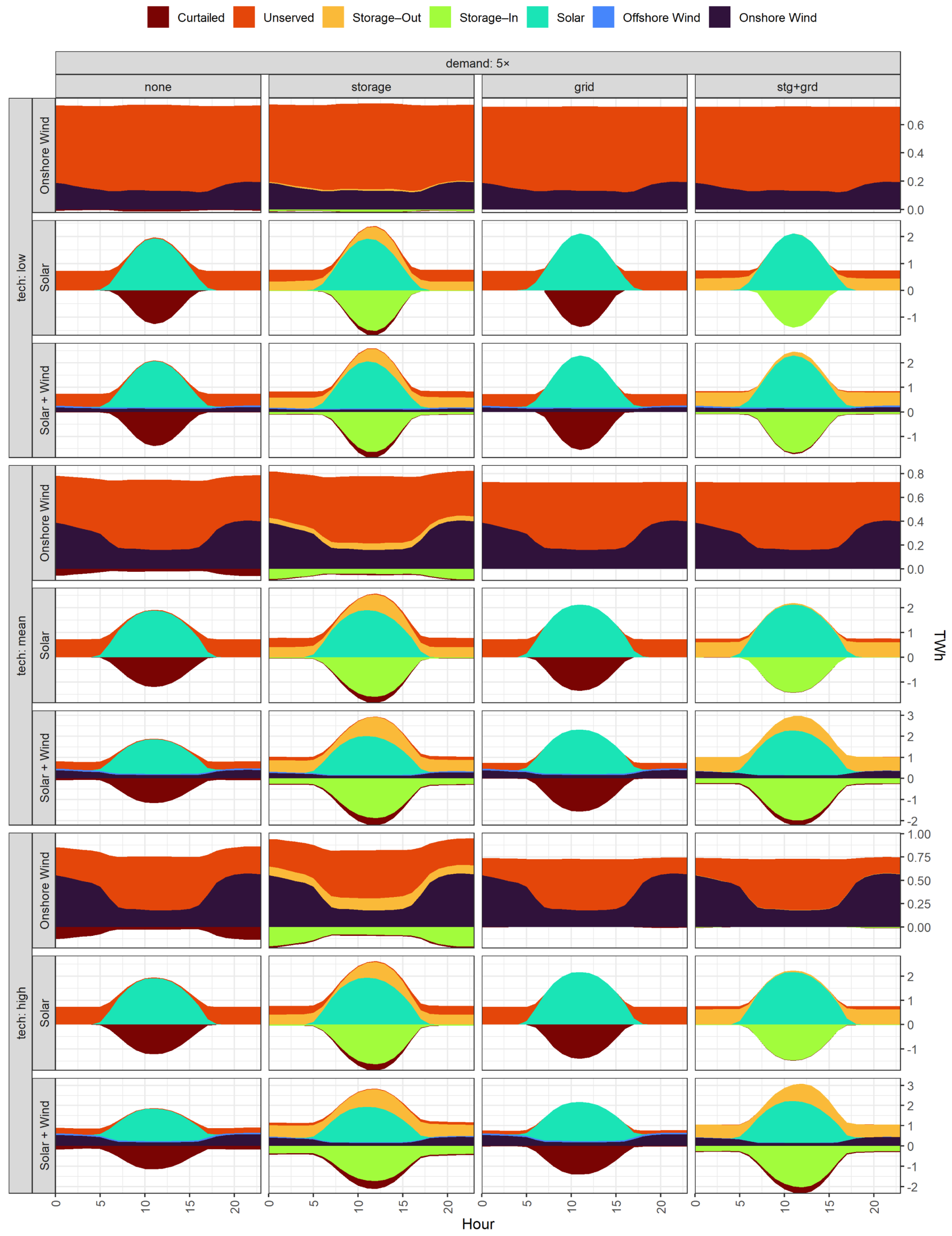
Figure 7 shows simulated intraday generation profiles and operation of storage for scenarios with demand equivalent to 2019 (‘1×’) and different sets of generating and balancing technologies (for the full set of scenarios, see
Figure A16,
Figure A17,
Figure A18 and
Figure A19 in the
Appendix A). The figure reinforces already-formulated findings and adds intraday insights into system operation by scenario. An interesting observation is that the combination of wind and solar energy without any balancing technology can still satisfy most of the final demand by doubling the generation capacity, with the expense of losing half the generated electricity (see column ‘none’, row ‘solar + wind’, and ‘curtailed’ states for curtailed supply of electricity). Individually, solar or onshore wind delivers roughly 50% of required load. Adding storage or grid reduces the system failure to serve the load (see ‘unserved’ load in the figure) and system inefficiency (‘curtailed’ energy). Both balancing options make all versions of the system quite reliable, with 95–100% of served load. Scenarios with combined solar, wind, storage, and grid show minimal overproduction without failing to serve demand.
Notably, the scenario with solar, wind, and grid shows only minimal unmet load, suggesting that spatial balancing can be used to design 100% of solar and wind systems able to serve the given ‘FLAT’ load. Wind energy plays a more significant part in spatial balancing, while solar energy requires more storage for intraday balancing. In scenarios with all generation technologies available, solar and wind energy compete based on cost, accounting for the balancing options. The ‘stg+grid’ scenario has a much lower share of wind energy than without any balancing options (‘none’) or grid-only scenarios (‘grid’), suggesting that wind energy with grid is more expensive than solar with storage. Changing these relative prices in the model will lead to different shares between the sources of energy.
Serving a fixed flat load with intermittent energy sources requires significant balancing capacity in terms of storage and interregional grid. Both technologies are either expensive or hard to deploy. Managing demand can be another option of balancing.
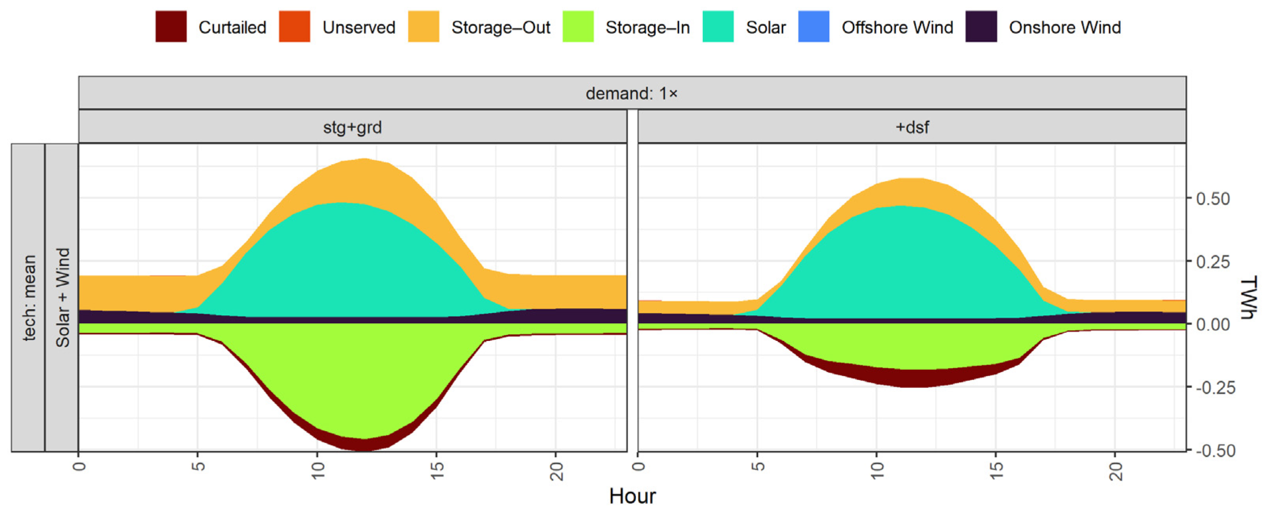
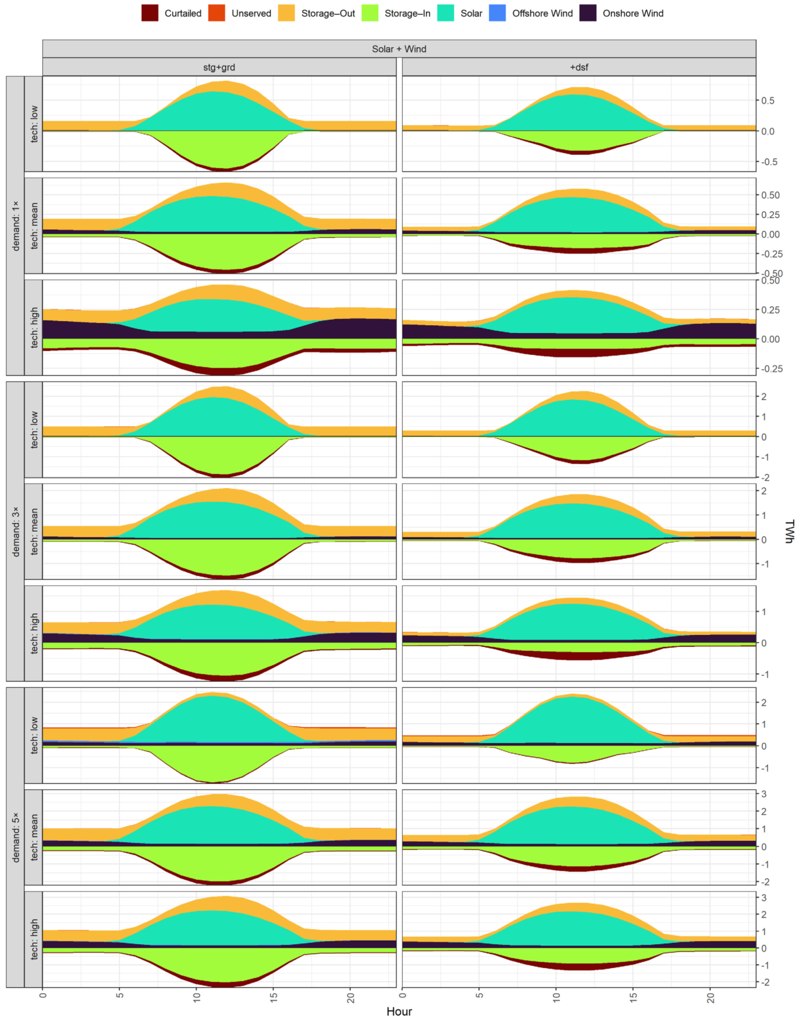
Figure 8 compares the ‘solar + wind’ and ‘stg+grid’ scenarios from
Figure 7 with the additional demand-side flexibility option (‘+dsf’).
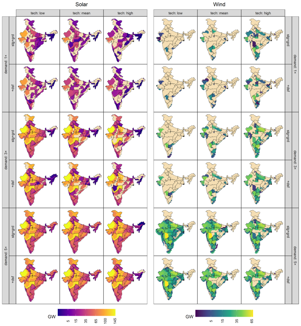
Figure A15 in the
Appendix A shows the optimised region-wise clustered generating capacity of solar and wind energy sources by scenarios without and with responsive demand options (‘stg+grd’ and ‘+dsf’, respectively). The partial flexibility of the load within a calendar day is more consistent with the solar cycle and thus can significantly reduce storage. While the wind capacity is lower in the scenario, the total gigawatts of the grid stays about the same (see
Figure 5).
3.2. Seasonality and Storage Duration
Along with intraday cycles and fluctuations, solar and wind energy potential varies throughout the year. This intermittent nature is harder to address with short-term storage and grid, and requires long-term storage, backup capacity, or interpersonal demand-side management.
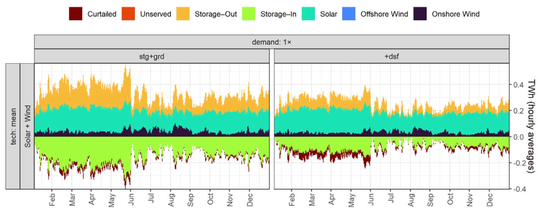
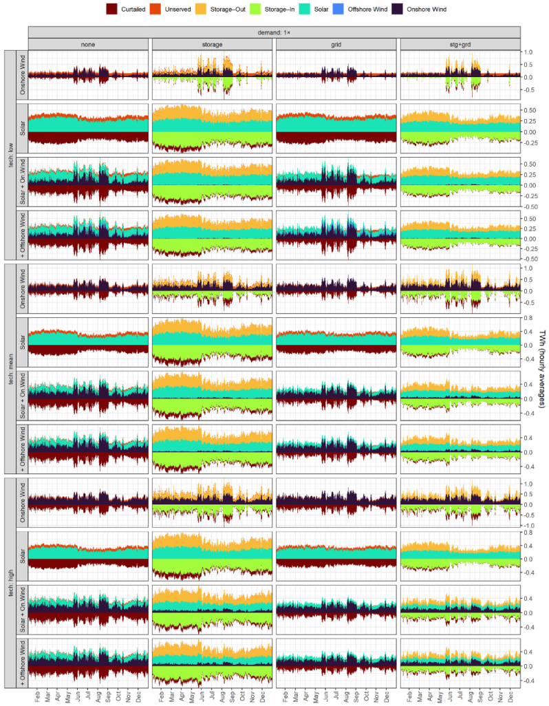
Figure 9 summarises the annual generation and balancing profiles for two scenarios (for all scenarios, see
Figure A20,
Figure A21 and
Figure A22 in the
Appendix A).
Even if the mixture of solar and wind capacity from different clusters is optimised to make fluctuations as minimal as possible to meet the fixed (‘FLAT’) demand in the first scenario in the figure (‘stg+grd’), the fluctuation of both wind and solar energy by day is significant. Wind energy is more variable and shows (in 2020 data) several months with double the production of the yearly average. Still, the system is optimised to accommodate such fluctuations, and curtailments are quite low throughout the year in this scenario. Interestingly, the scenario with the additional balancing option on the demand side (‘+dsf’) shows a higher level of curtailed energy, most likely due to lower storage.
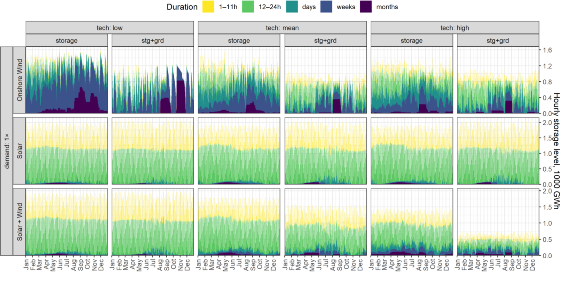
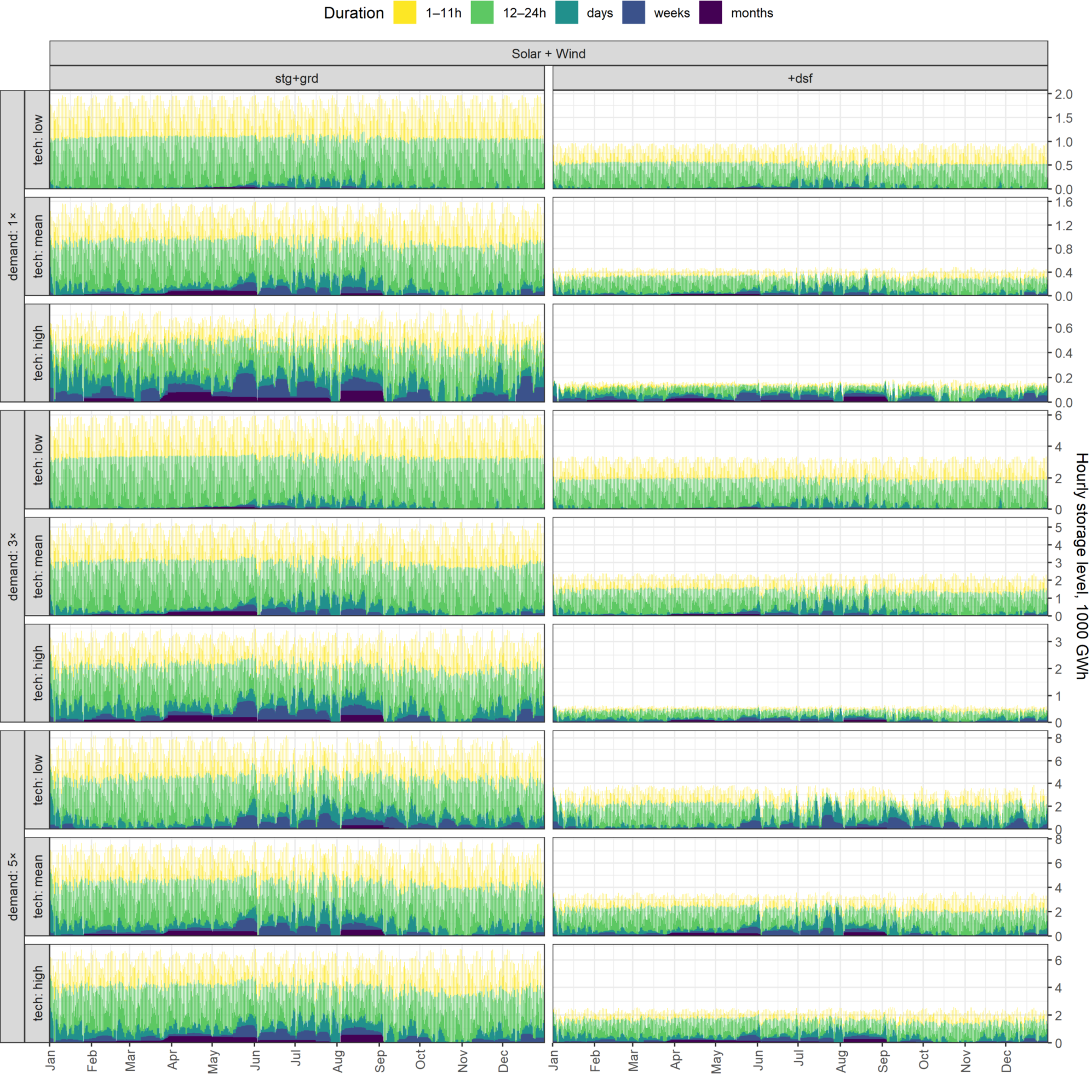
Figure 10 shows decomposition of the storage level by duration of charge in scenarios without demand response at the ‘1×’ demand level (see
Figure A23 and
Figure A24 for all other scenarios). Onshore wind in all technological optimism scenarios requires long-term storage: weeks and months to deliver electricity during shortage seasons, mostly from August to November. For lower wind hubs (‘tech: low’), more storage capacity is required of longer duration due to the more intermittent nature of wind speed at lower heights.
In solar-only scenarios (‘solar’), storage is used mostly for intraday balancing. The need for longer-term storage levels is low and further reduced if combined with grid. The finding that grid reduces long-term storage usage is consistent with Gulagi et al. [
22]. With solar and wind energy combined, storage capacity is drastically lower in 150 m hub scenarios with available grid (compare ‘stg+grd’, ‘tech: high’, and ‘solar + wind’ scenario on
Figure 10 vs all other). This 2.5-fold drop in storage capacity indicates higher intraday complementarity of estimated wind at 150 m with solar energy. As discussed in the Data and Methods Section (see also
Figure A3 and
Figure A25 in
Appendix A), the extrapolated wind speed for higher altitudes requires validation with real measurements once available.
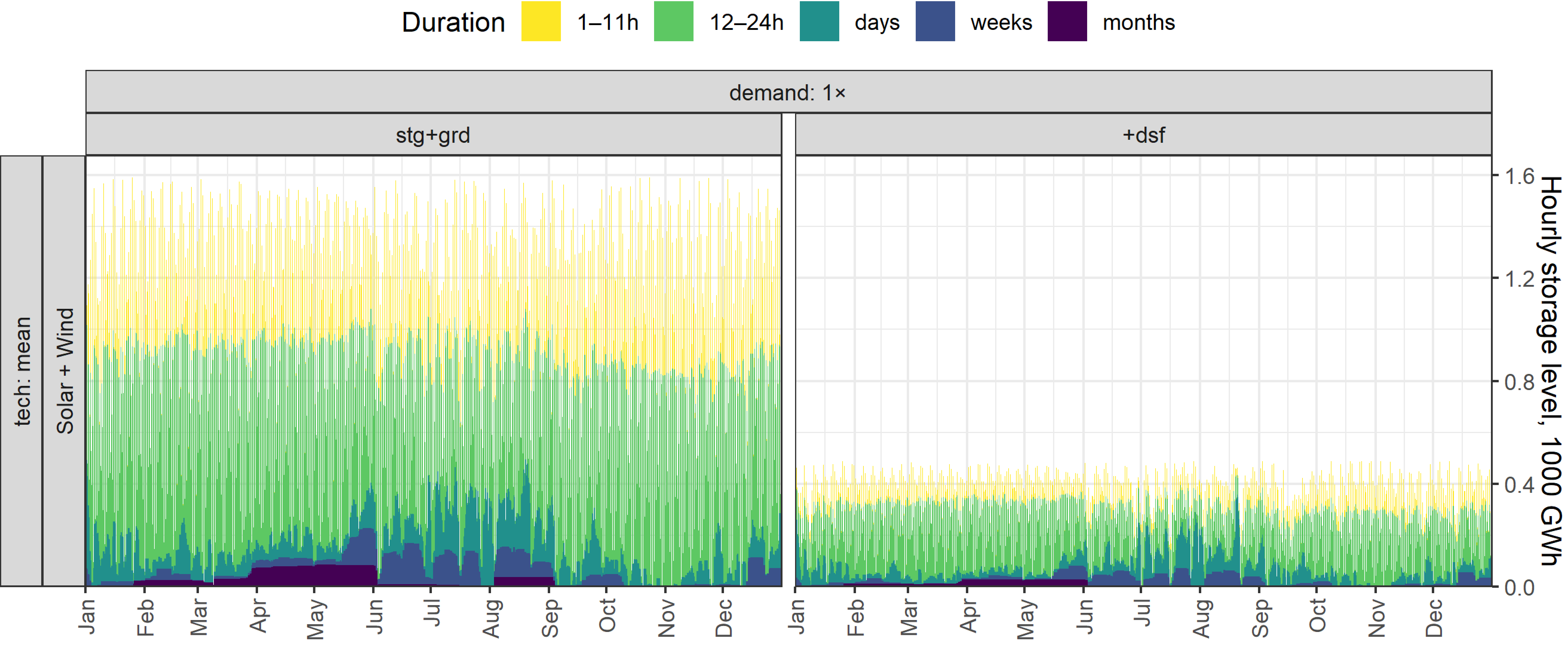
The need for intraday balancing might be significantly reduced with demand-side flexibility.
Figure 11 shows the decomposition of the storage level by duration of charge with and without demand response (see also
Figure 8 and
Figure 9 for the same sets of scenarios and
Figure A24 for all others). With the addition of demand-side flexibilities (‘+dsf’ vs ‘stg+grd’), the storage level reduces a further three to fourfold. Although a little less electricity is produced, around 50% of it is consumed during the daytime, due to the ability to partially adjust the load curve to the supply—basically, the solar generation cycle. As a result, the requirement for intraday balancing is significantly lower. The total hourly storage in the scenarios is still quite high, exceeding 400 GWh. However, this example demonstrates the potential for further reduction in storage needs if demand can be managed. Managing load by season can further reduce the need for long-term storage.
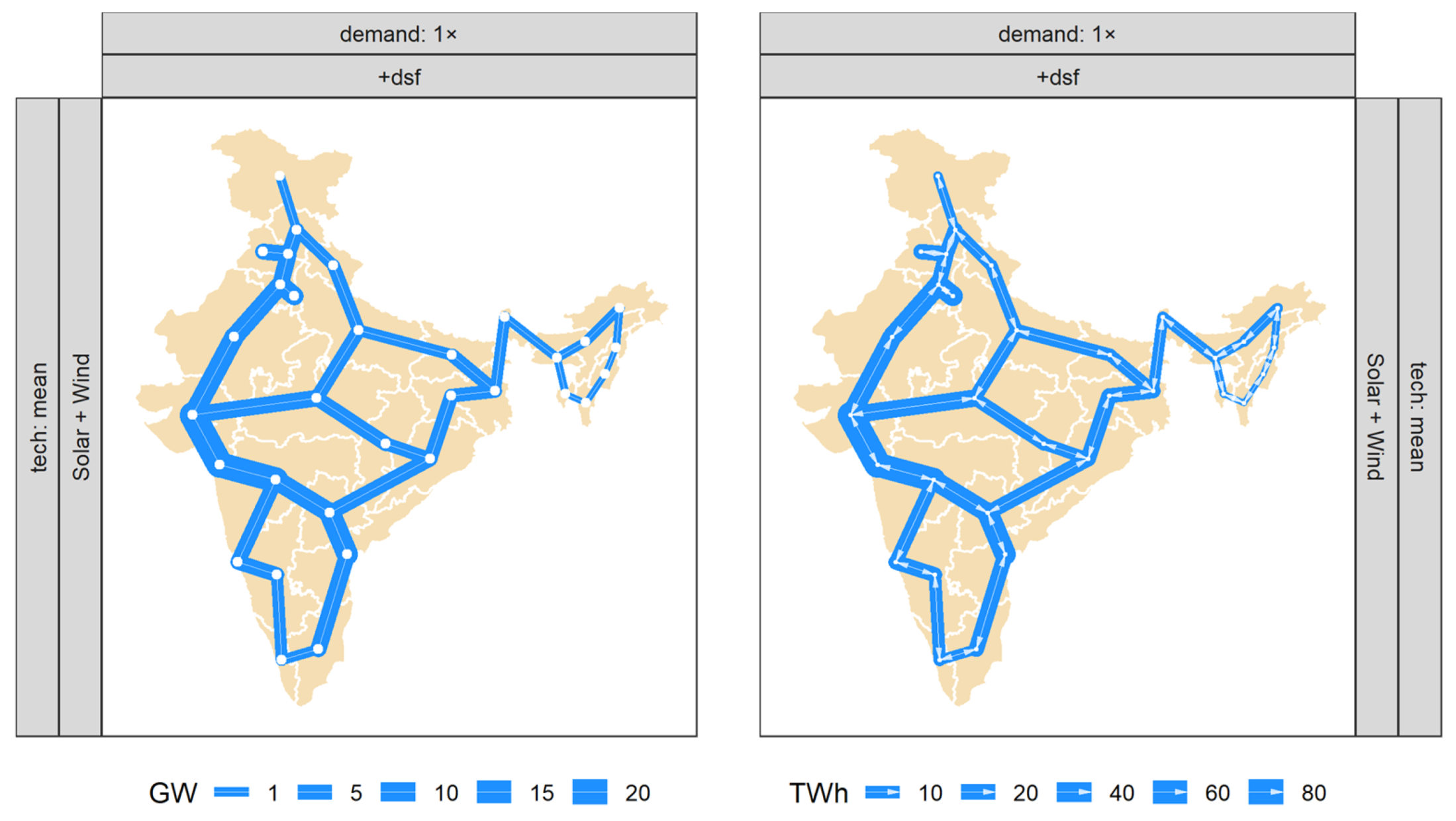
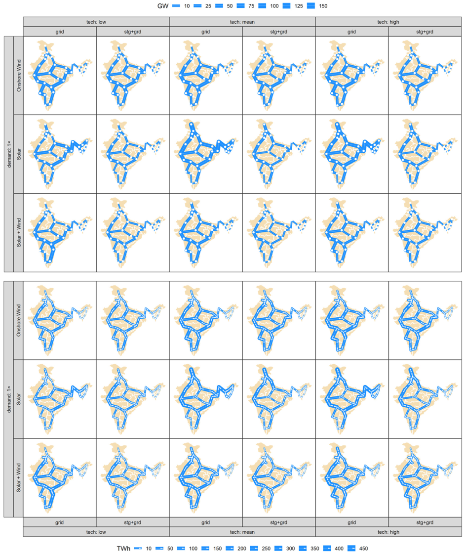
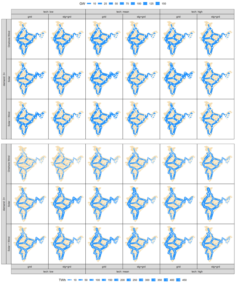
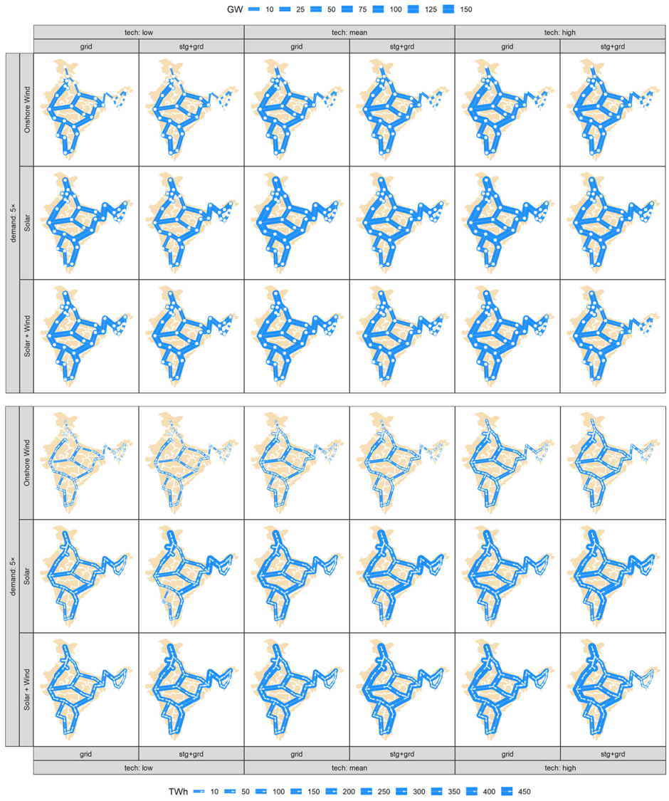
3.3. Interregional Trade
Spatial balancing has been shown to be important in all scenarios.
Figure 12 depicts the interregional grid capacity and annual trades for the ‘1×’ demand level, scenarios with all considered generating and balancing options, and average technological assumptions (see
Figure A26,
Figure A27 and
Figure A28 in the
Appendix A for all scenarios with grid).
All 36 power lines were selected for investment in all scenarios with grid technology. Though the total capacity and each power line differed significantly by scenarios, scenarios without storage tended to use more grid for spatial balancing. In scenarios with wind energy only, the size of the power lines was more uniformly distributed across the country, with lower-capacity connection in the east and north. Grid in solar-only scenarios without storage tends to have ‘heavier’ power lines to the east, while storage shifts the main capacity to the north–centre–south connection. Gujrat and Karnataka showed maximum grid capacity through most scenarios due to the high potential of wind and solar resources in the regions and high consumption.
The overall sizing of the long-distance grid was quite high in all scenarios. The lowest grid capacity can be observed in scenarios with flexibility on the demand side.
Figure 12 shows such a case, where maximum capacity between two regions is 20 GW, which is equivalent to several high-voltage AC or two modern high-voltage DC power lines. Certainly, the shape of the considered grid used to identify the benefits of interregional exchange is quite simple. Further studies may address a more complex network.
3.4. Demand-Side Flexibility
The ability to manage the load curve at least partially can be a huge benefit for a high-renewable power system in India. Scenarios with demand response show much lower storage and grid (see
Figure 11 and
Figure 12 and Discussion).
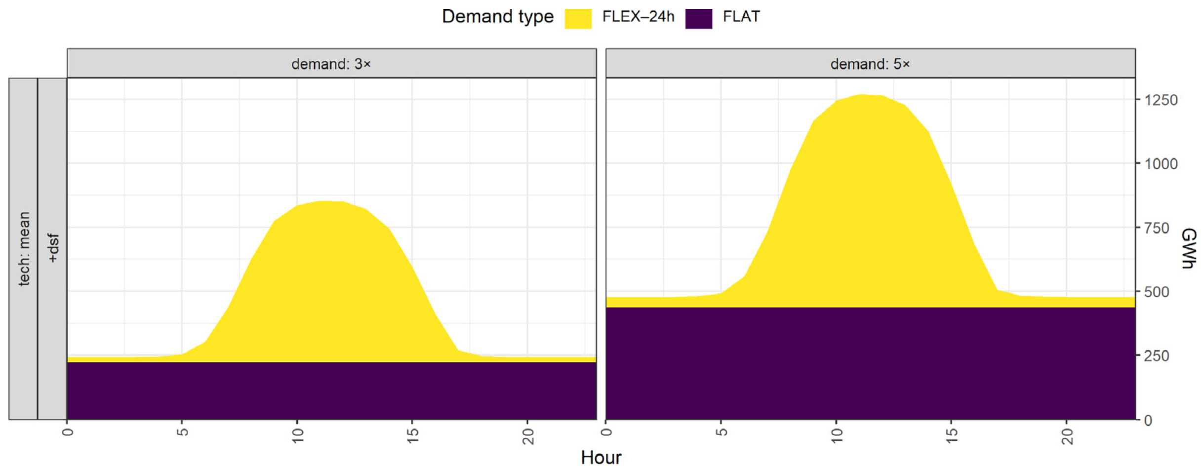
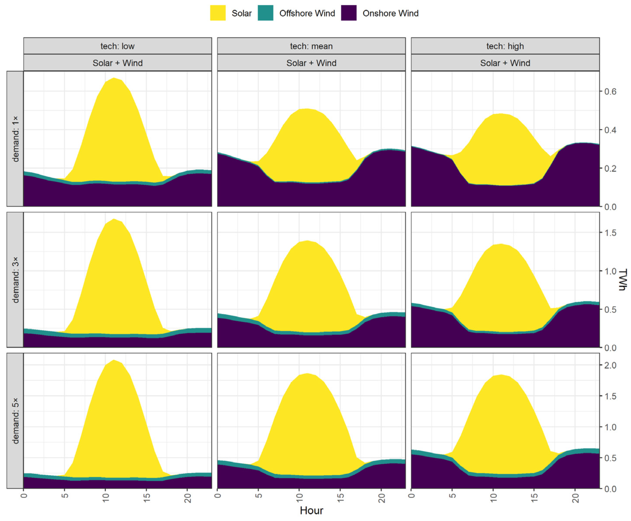
Figure 13 shows demand structure by hour for two scenarios, solved on 41 years of weather data (see
Table 1). The load in the scenarios is split into two technological groups: ‘FLAT’ and ‘FLEX-24h’.
The ‘FLAT’ part of the demand is a fixed load, similar to the base-load definition in power systems. This technological group consumes the same amount of electricity 24 h, 365 days in every region. The FLEX-24h group has the same load for every day of a year, but the time of consumption within a day can vary, which is optimised by the model. As described in the Data and Methods Section, we assumed a two-level electricity market with different pricing for ‘FLAT’ and ‘FLEX-24h’ types of electricity supply. The ‘FLAT’ load can pay higher prices and based on the different assumptions regarding the electricity costs in each group and region, the model optimises both the power system and the load curve to achieve the lowest possible system costs.
We also added constraints on the ‘FLAT’ group to ensure some base load in every region. The ‘5×’ scenarios also had a national constraint on the ‘FLAT’ load type, which ensured nationwide sharing of the ‘FLAT’ load, but the ratio was optimised by the model for every region.
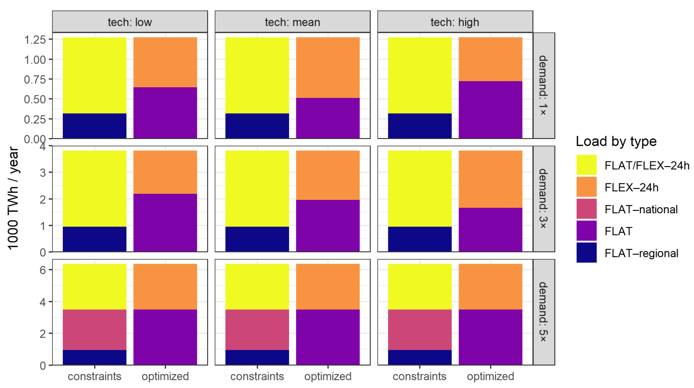
Figure 14 summarises the imposed constraints and optimisation results for each ‘+dsf’ scenario.
As follows from the figure, the resulting share of the ‘FLAT’ load is much higher than its lower constraint (FLAT-regional) in all 1× and 3× demand scenarios. This result is a function of relative prices (or credits) exogenously introduced to the scenarios. A higher price (credit) for ‘FLAT’ electricity will force the system to build more alternatives to flexible load-balancing technologies (storage and grid) to sell more electricity to the ‘FLAT’ load. Lower ‘FLAT’ prices will reduce its competitiveness, and more ‘FLEX-24h’ load will be used to substitute expensive storage and grid use.
Scenarios with the highest demand level (‘5×’) have an additional constraint that requires the total ‘FLAT’ load to be at least 55% nationwide, with a 15% minimal share in every region. Even the pricing methodology is the same as in the ‘1×’ and ‘3×’ demand levels The actual share of the ‘FLAT’ load is at its constrained level. A probable explanation here is the lower potential share of wind energy in total production, since the wind resource is already reaching its upper limit in ‘3×’ scenarios.
3.5. Levelised Costs of Energy
Technological cost assumptions in this study are quite simplified and do not vary across model regions and clusters. However, generation and balancing capacity mixtures in scenarios, overcapacity that leads to energy losses, and unmet demand are very different and should have different economic value.
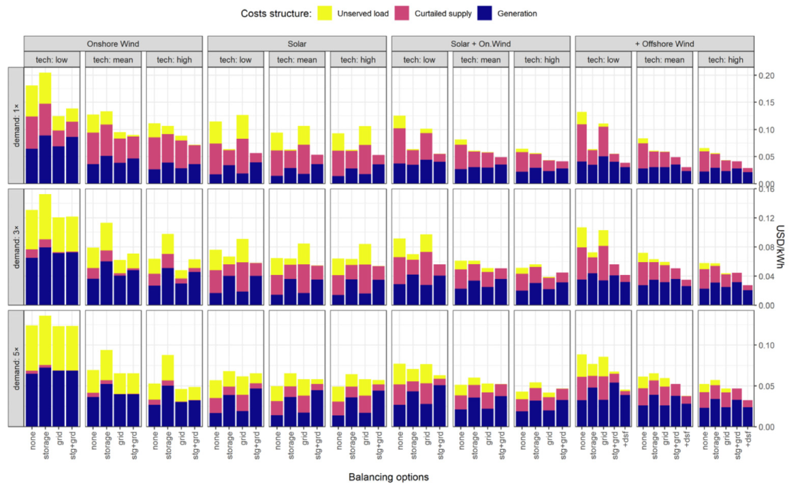
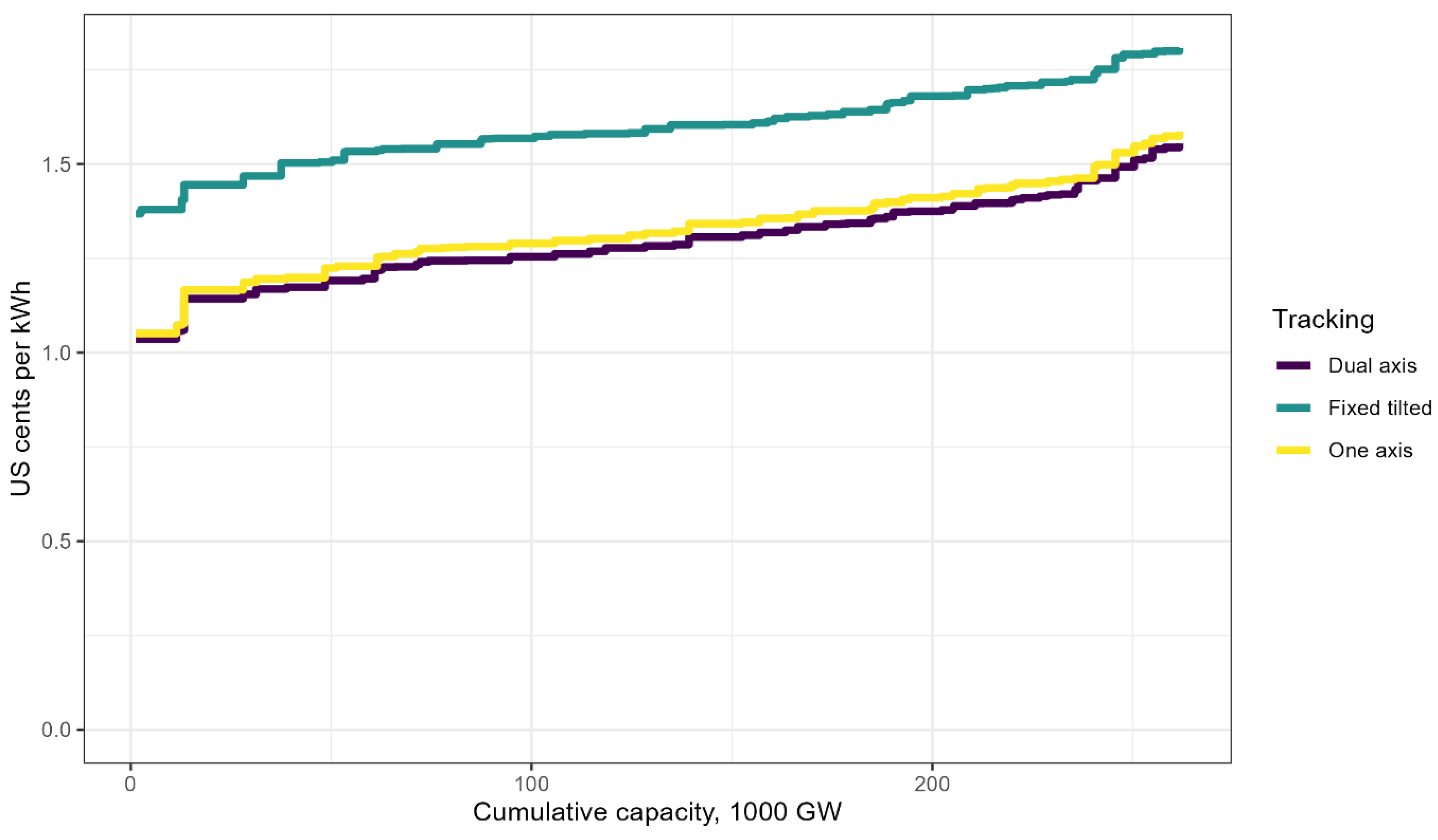
Figure 15 characterises economic metrics of the 153 scenarios: the levelised costs of electricity (LCOE). We split these costs into several groups. The ‘Generation’ bar indicates the costs of electricity production, distribution (long-distance grid only), and balancing. Solar energy is the cheapest energy source in the study. Therefore, scenarios with solar energy only (‘Solar’) and no balancing (‘none’ on
x-axis) show the lowest costs of energy per kilowatt hour. Wind energy is roughly two to four times more expensive than solar, and the difference is lower for higher technological optimism (‘tech: high’). This explains the tendency towards more solar energy in scenarios with both energy options.
‘Curtailed supply’ in the figure indicates energy losses, with an overbuilding of the generation stock to meet demand in hours and regions when electricity production is low or not available and the overbuilding being less expensive than balancing options available in the scenario. The costs of curtailed energy are estimated as generation costs per consumed electricity. Some curtailed energy exists in all scenarios, except those where the power system fails to deliver a significant part of the demand (see ‘Onshore wind’, ‘demand: 5×’ scenarios).
The costs of ‘Unserved load’ in the figure are indicative. To show the magnitude of the system’s failure to deliver electricity when needed, we assumed that the costs of undelivered electricity were 50% higher than generation + curtailed costs. (In the optimisation, the cost of unmet load is USD 1/kWh for all scenarios.) Scenarios with unmet load have used all available options to meet demand, and rejecting the delivery for some hours was the cost-optimal solution for the technological options considered. Existing unmet load indicates that the system has reached its potential to meet demand and additional technological solutions are required to avoid cutting off the demand.
The comparative figure shows several trends. First, more technological options on the generation or demand side reduce system inefficiency and lower the cost of electricity. Using just the complementarity of wind and solar energy without any balancing technologies gives roughly 5–10 US cents/kWh of delivered electricity, depending on demand and technological optimism. Adding storage and grid is sufficient to deliver all demanded electricity in almost all scenarios and pushes the levelised costs below 5 cents/kWh in all scenarios except 5× demand with low technological optimism. Scenarios with demand-side flexibility (+dsf) show the lowest supply costs: 3–4 cents/kWh.
3.6. Long-Term Optimisation
Renewable systems are weather-dependent, 100% renewable depend entirely on weather and balancing capacity. By selecting one weather year for optimisation of the power system, we assume that weather patterns observed that year would repeat or not change significantly in future years. Solar cycles and rainy and windy seasons are well known and represent a significant part of variability in energy sources. However, the weather patterns do not repeat themselves exactly, and optimisation based on one weather year will shape a system that is most consistent with that particular year’s solar and wind energy availability. Longer-term optimisation with several years of weather data will shape a system that is consistent with multiple years of weather data. Additionally, more years of data will more likely capture rare weather events of prolonged intermittent nature that can cause blackouts.
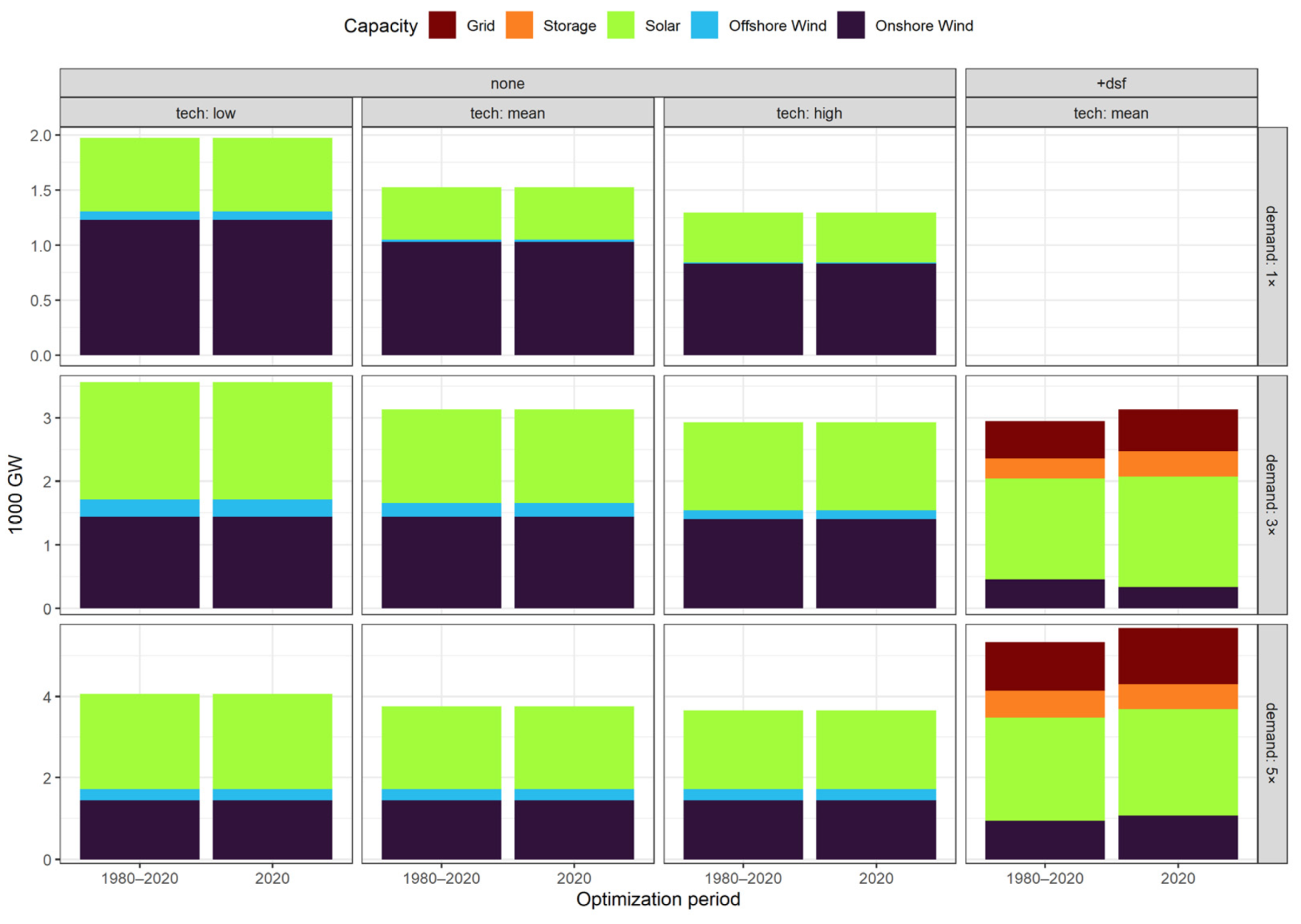
In this study, we picked 11 of 153 scenarios to optimise the structure of the power system using the full 41 years of hourly time-series data available in MERRA-2.
Figure 16 compares the capacity structure optimised based on 41 years of weather data at once (1980–2020) with 1-year data optimisation (weather year 2020). Nine of the scenarios had no balancing options to evaluate pure complementarity of wind and solar generation on long-term data. The two additional scenarios (‘+dsf’) had all generation and balancing options.
As follows from the figure, the 41-year optimisation shows overall lower capacity than the 1-year optimisation. The result might be surprising, because multi-year optimisation should pick a capacity that is consistent with all-weather years, and different weather events may affect capacities in regions. However,
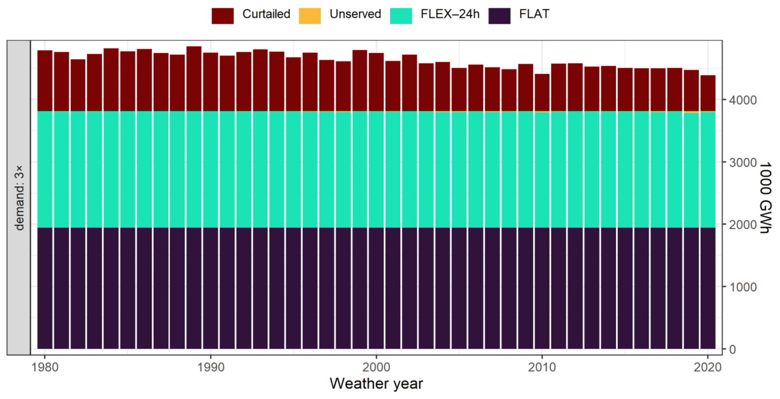
Figure 17 indicates that 2020 had the lowest total generation and curtailed energy through all 41 years of data, suggesting that it had the lowest total production (the hight of columns). The figure also shows that the demand structure can be consistent throughout the years. Flat and flexible demand have the same level for all weather years, with the exception of the small unmet portion in several years. This can potentially be managed by adding reserve capacity, storage, backup capacity, or additional demand management.
As an additional observation, overall generation (solar and wind energy) has been declining slightly since the mid-1990s. This phenomenon might be related to climate change, growing air pollution, MERRA-2 data methodology and assumptions, other factors, or could just be random. This should be addressed in future studies.
3.7. Transitional Dynamics
The macro-energy modelling scenarios indicate that a wind- and solar-based power system can be affordable, reliable in delivering electricity with all existing intraday variability and seasonal variations, and consistent with long-term weather profiles. Further research should address precise locations for installations of generating capacity, evaluate feasible limits of storage and long-distance grid, access the potential for demand-side flexibility, and address short-term balancing and grid stability. Assuming that high- or full-renewable systems will be deployed, it is important to start planning the transition of the power system from traditional thermal-dominant generation to zero-carbon renewables.
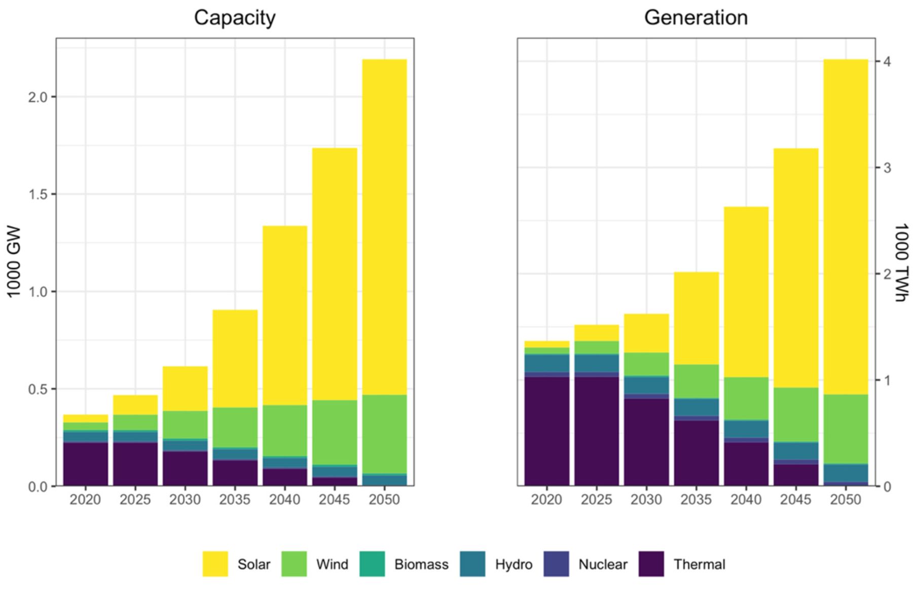
In this section, we evaluate a possible transition pathway, sketching the required steps by decades, assuming all fossil fuel-based generation will be replaced by solar and wind energy by 2050. For simplicity, we keep small and large hydro, nuclear, and bioenergy at the same levels as in 2020. We consider one transitional scenario where the final demand reaches triple the level of 2019 (3800 TWh) plus actual generation by hydro, nuclear, and biomass energy (200 TWh) for a total of 4000 TWh annual demand.
To evaluate the transition with the IDEEA model, we pick one of the scenarios as targeted (‘demand 3×’, ‘tech: mean’, ‘+dsf’; see
Figure 16) and fix solar, wind, grid, and storage capacity as a 2050 target on top of hydro, nuclear, and biomass capacities, which stay constant through the transition. The base-year capacity is fixed at the 2020 level. The growth in final demand is assumed to be exponential for simplicity. The fossil-based generation stock is assumed to retire gradually from 2025 to 2050.
Figure 18 shows the result of optimisation of the transition from the base year to 2050.
4. Summary and Conclusions
In this study, we explored a potential transition of the Indian electric power system to carbon neutrality around mid-century, relying solely on intermittent renewables. We intentionally limited all energy supply sources to wind and solar to evaluate the structure and features of a 100% renewable power system, the potential of complementarity of the energy sources across locations, and the role of alternative balancing options going beyond energy storage. We used 41 years of reanalysis weather data (MERRA-2) to study complementarity originally from 1200 locations across India and 100 km offshore. The data were grouped in spatial clusters based on similarity, using long-term correlations within neighbouring locations separately for wind and solar energy for every model region. The resulting 114 wind energy and 60 solar energy clusters were used as inputs for the IDEEA model.
The installation potential of solar photovoltaic systems and wind turbines for every cluster was defined by area, estimated on GIS information. We assumed that up to 10% of every territory could be used for wind turbine installations and up to 1% of the area in every solar cluster for photovoltaic installations. We did not locate where the installations would happen in every spatial cluster. Instead, we assumed that the defined share of every cluster was suitable for the installations, using the land directly or combining with other economic activities, such as agriculture for wind turbines and buildings or highways for photovoltaics.
We developed a 153-scenario matrix with four dimensions (branches) of varying settings to evaluate every generation source, complementarity between them, and the role of alternative balancing options under different technological assumptions. The variety of scenarios outlined the boundaries of potentially feasible solutions for a 100% renewable electric power system in India. Unmet load was used to characterise the system’s failure to satisfy demand and curtailed energy as the system’s inefficiency. System-wide levelised costs of electricity were evaluated for every scenario as an indicator of economic efficiency.
Scenarios with one generating technology assessed the potential of wind or solar energy as the dominant energy source in the system and the required balancing options. A wind-dominated power system can potentially be deployed in India, along with a significant expansion of the interregional grid and long-term storage. Even with the high seasonality of wind energy, long-term storage (or back-up capacity) makes the system technically viable. The scattered distribution of the resource around the country and different generation profiles among locations highlight the role of the long-distance grid for distribution and balancing.
A solar-dominated power system requires the deployment of intraday storage to serve the load through the night hours. Expansion of the grid diversifies the resource across regions, takes advantage of relatively higher solar potential in several regions, and reduces storage. As a result, solar energy has much higher overall potential than wind. It can technically meet a fivefold increase in demand for electricity (with 1% upper bound on land use in clusters). In contrast, wind energy reaches its potential at around the 2019 consumption level (under the given assumptions).
Roughly half the load can be served if only one of solar or wind energy is considered with no balancing. A mixture of the two technologies can be proposed to satisfy 75–90% of fixed ‘FLAT’ demand, even without any balancing technologies, highlighting the complementarity of wind and solar energy. However, no balancing leads to high energy losses: total generation is twice the demand, and half of the produced electricity is curtailed. Energy storage and long-distance grid minimise the unmet load to zero and curtailed energy to 5–10% of annual generation.
Serving ‘FLAT’ demand with variable energy sources requires significant expansion of energy storage and long-distance grid. The total capacity of storage and grid in the scenarios with two balancing options are comparable to generation capacity. It might be challenging to deploy such a massive infrastructure. Additional balancing options, such as the ability of demand to at least partially adjust to intermittent supply, can potentially substitute a significant part of storage and grid capacity.
To demonstrate the value of flexibility on the demand side for 100% renewable systems, we split the total load into two demand-side technologies with different requirements for supply. The first group still required a non-intermittent constant in time load through the year. The second group can potentially adjust electricity consumption within a day if the total daily supply is met. To distinguish the two types of electricity within the model, we developed a two-level electricity market structure with different price signals for the demand groups. Since constant in-time electricity requires more balancing infrastructure, it should have higher market value to compete with the partially flexible load.
Based on the results, 40–60% of the intraday flexible load in total consumption can reduce storage requirements from three- to sixfold, depending on the type of scenario, and reduce system-wide levelised electricity supply costs by up to 40%. The curtailed electricity is still not zero but can potentially be addressed by further consideration of seasonal optimisation of load.
One of the critical questions in designing a high-renewable system for India is the availability of wind power. Our estimates show that higher hubs (100–150 m) may have significantly more potential and complementarity with solar energy. Moreover, scenarios with higher technological optimism demonstrated a substantially higher share of wind capacity and storage reduction favouring a long-distance grid. However, such extrapolation-based estimates should be confirmed by direct measurements and further studies.
Long-term reliability is a major concern for intermittent renewables. Rare weather events with low solar and wind energy availability may lead to severe blackouts in the electricity supply. In this study, we solved several scenarios using 41 years of weather data to evaluate the long-term complementarity of solar and wind energy and optimise the power system that can function in alternative weather years. The resulting capacity structure of the 41-year optimised power system was slightly different from the 1-year optimisation. Surprisingly, the extended period of weather data suggests lower total wind and solar energy capacity than the 1-year optimisation using 2020 weather data. Based on MERRA-2 data, 2020 had the lowest wind and solar energy potential vs 1980–2019. The data showed a visible negative trend in generation from the 1990s to 2020 for both wind and solar capacity. This phenomenon might be related to climate change, more air pollution, other factors, or could just be random, and should be addressed in future studies.
Our analysis reinforces the earlier findings of the potential feasibility of 100% renewable system for India using more granular and long-term weather data, and sensitivity analysis of the results to the uncertainties in the data. Our results suggest that a two-energy system with solar and wind energy only can deliver fivefold the annual demand of 2019, and that robust, reliable supply can be achieved in the long term, as verified using the 41 years of weather data.
Based on the findings, India can more confidently consider a higher share of renewables in power generation. Advanced interregional power grid and demand-side flexibility have great potential in balancing intermittent renewables and limiting the expansion of expensive energy storage. Further studies can add more details by considering more energy sources and resolving data uncertainties. Additional energy sources, including hydro energy and biomass, can further complement and reduce the required balancing infrastructure. Hydro energy already plays a significant role in India: reservoirs accumulate water during the monsoon season for the whole year and can potentially be a source for seasonal and intraday balancing. The potential of wind energy on higher hubs, land for photovoltaic system and wind turbine installations, a more detailed power grid, optimisation of locations of new demand, and seasonal flexibility of final demand are potential directions to improve understanding of India’s renewable future.


 ,
, 


