An Analysis of the Operation of Distribution Networks Using Kernel Density Estimators

Abstract

Efficiency in the operation of distribution networks is one of the commonly recognised goals of the Smart Grid aspect. Novel approaches are needed to assess the level of energy loss and reliability in electricity distribution. Transmission of electricity in the power system is invariably accompanied by certain physical phenomena and random events causing losses. Identifying areas where excessive energy losses or excessive grid failure occur is a key element for energy companies in resource management. The study presented in the article is based on data obtained from distribution system operators concerning 41 distribution regions in Poland for a period of 5 years. The first part of the article presents an analysis of the distribution of values for the introduced energy density and energy losses in the lines of medium- and low-voltage networks and in transformers supplying the low-voltage network. The second part of the article presents the assessment of the network reliability of the same distribution regions based on analysis of the distributions of System Average Interruption Duration Index (SAIDI) and System Average Interruption Frequency Index (SAIFI) values for planned and unplanned outages. Data analysis is performed by non-parametric methods by means of kernel estimators.

1. Introduction

Implementation of European Union provisions in the field of energy efficiency are focused on increasing energy security, counteracting climate change, and should also have a positive impact on the economy through the development of the market for new services and innovative energy technologies [1]. The improvement in energy efficiency can be achieved in many ways, one of which is to reduce electricity losses in distribution grids [2,3], to construct smart micro-grids [4,5], to carry out a stochastic loss analysis approach for distribution systems [6], to assess reliability of renewable energy interfaced distribution system taking into account loss minimisation [7] or to integrate of wind power and energy storage with the bulk power system [8].

Distribution grids are the final element of a complex power system. Their work is influenced by a huge number of factors, many of which, including the most important ones, are random. It is therefore advisable to analyse the operation of distribution networks using appropriate statistical methods, taking all these factors as random variables. Such analyses are necessary, for example, in order to define a strategy for the development and modernisation of distribution networks. Due to the complexity of the problem, its degree of difficulty and labour intensity, the works on this issue are usually academic in nature. These studies often discuss theoretical foundations and present mathematical models without reference to specific networks [9].

In addition, it should be noted that distribution networks are dynamic, both in terms of their structure and installed devices, as well as in terms of their load or the environmental conditions in which they operate. Therefore, modelling the entire distribution system does not make much sense because the obtained results will always be burdened with many simplifying assumptions, and accordingly, also with significant errors. It is advisable for distribution companies to carry out practical analyses of real networks based on the available data so that actions can be taken to improve their functioning.

Many tasks of designing the development of the distribution network or the assessment of working conditions are generally based on the results of estimation determined for the most difficult working conditions. State estimation in relation to power systems consists in estimating the complete set of information about the system operation regarding generation, voltage and load values in all nodes of the distribution network. Apart from the state estimation task [10,11,12,13,14], there is also a narrower problem concerning the estimation of loads [15,16]. The estimation methods are based on computational methods in which statistical models [17,18], the theory of fuzzy sets [19], artificial neural networks [20] or hybrid algorithms combining various computational techniques, such as neural networks and fuzzy logic [21], as well as methods of optimising particle swarms with elements of genetic algorithms, are most often used [12,22]. In the area between the analytical and statistical approaches, there are methods that combine elements of both computational techniques. They constitute a practical compromise, often adequate to the current national realities of distribution systems, between the amount of input data needed for calculations and the accuracy of the results of power and energy losses [23,24,25]. These methods, which could be described as hybrid, use the information available in the energy reporting on energy flows through individual groups of distribution network elements and substitute network models. Based on such methods, it is possible to build a methodology supporting the analysis of the operation of distribution networks [20,26,27].

The issues related to the reliability of power system operations are currently generating great interest all over the world. Many works have been devoted to this subject—both experimental and theoretical. In the subject literature, the reliability of the power system is significantly related to the name of Roy Billinton, who together with a group of co-workers published many articles and books, e.g., [28,29,30,31,32]. Usually, the reliability of the generation, transmission or distribution subsystem is analyzed independently [33,34,35,36]. Reliability calculation methods can be generally divided into analytical, consisting in the analysis of random events or processes; simulation (Monte Carlo, statistical modelling), consisting in simulating random events and processes; mixed (combined), which is a combination of analytical and simulation methods [37].

It is often necessary to select the appropriate method for a given task. It may turn out that for some problems the use of one method turns out to be insufficient and there is a need to use other methods, more effective for a given class of problems. In [38] a number of problems and challenges which researchers in reliability engineering are facing when analysing complex systems were shared. In [39] problems in the reliability planning of electric distribution networks were treated as multiobjective issues, consisting of the minimisation of three objective functions. In the literature on reliability, we can find many different methods of analysis, for example using a discrete particle swarm optimisation [40,41], using a fuzzy-based analytical and a fuzzy-based Monte Carlo simulation technique [42] or using a nonparametric estimator [43]. Whereas in [44] in an interesting way the history of reliability engineering was presented. For one of the ways to effectively formulate and solve tasks related to the analysis of the power grid operation is non-parametric statistics methods, in particular the Kernel Density Estimation (KDE) application.

1.1. Energy Losses in Distribution Networks and Transformers

The flow of electric current through the distribution network is inherently associated with the loss of power and energy in it; active on element resistances, reactive on reactances, both of which are harmful. The energy to overcome losses must be generated in power plants, which requires the expansion of equipment and the use of correspondingly more fuel for its production. These losses have to be passed on by all the system elements involved in the distribution of energy, which requires increasing its nominal transmission capacity. By converting to heat, in accordance with Joule’s law, losses cause heating of the leading current parts of the system components, forcing their respective dimensioning.

Balance grid losses (also referred to as the balance difference or balance losses) are the difference between the energy fed into the grid and energy received from that grid. Balance losses range from a few to several per cent of the volume of transmitted energy, and their size proves the technical and organisational level of the distribution company. The percentage distribution of energy losses in the distribution network in relation to the technical losses in the low-voltage (LV), medium-voltage (MV) and 110 kV networks, respectively, and to the balance losses in the distribution network for one of the Distribution System Operators (DSO) in Poland are given in

Table 1. Percentage distribution of electricity losses in the distribution network.

Network	The Place Where the Losses Arise	Technical Losses (%)	Balance Losses (%)
LV	in the electricity meters	26.32	2.22
	in the connections	13.83	1.05
	load on LV lines	58.49	7.27
	total technical in LV	100.00	10.66
MV	load losses in MV	62.43	30.16
	voltage losses in transformer MV/LV	25.29	13.41
	load losses in MV/LV transformer	7.73	4.21
	voltage losses in transformer MV/MV	0.20	0.09
	load losses in MV/MV transformer	0.06	0.03
	other voltage losses	4.29	1.88
	total technical in MV	100.00	49.78
110 kV	load losses in 110 kV lines	61.62	12.29
	voltage losses in 110/MV transformers	26.44	5.48
	load losses in 110/MV transformers	8.17	1.65
	other voltage losses	3.77	0.62
	total technical in 110 kV	100.00	20.04
LV + MV + 110 kV	total technical losses	80.48
	total commercial losses	19.52	19.52
	total in distribution network	100.00	100.00

.

Balance losses are the sum of technical (current + voltage) and commercial losses, which arise mainly in the LV grid. For domestic distribution networks, energy losses in the 110 kV grid account for approx. 20%, in the MV grid approx. 50%, and in the LV grid approx. 30% of all balance losses [2]. Technical losses account for about 80% of energy losses, commercial losses for 20%. Losses in MV are 30%, in MV/LV transformers it is 17% and in LV lines 7% which have the largest share in technical losses. Losses in 110 kV grid lines are 12% and in 110/MV transformers are 7%, which also have a large share. No analysis has been carried out for high-voltage networks as they are 100% reserved and work with the system network; thus, distributors are not always fully responsible for the optimal operation of these networks.

Losses in MV/LV transformers for a given distribution area will depend primarily on the power of the installed transformers. Transformers should be selected so that losses in them (load and no-load ones) are as low as possible. If the minimum energy losses in the transformers are taken as a function of the aim, then the optimal transformer load factor (peak) is 0.7 ÷ 0.8 [2]. For most distribution areas, the transformer load factors (peak) are 0.4 ÷ 0.5. Due to the lack of metering of the network, the exact value of the energy fed into the low-voltage network is not known; hence, the energy losses in these networks cannot be precisely determined. The load energy losses depend on many factors: the energy density, the length of the network lines, their cross-sections, cut-outs in the networks, or the aforementioned transformer loads. About 55% of energy losses in the distribution network occur in the lines of the LV and MV networks and in MV/LV transformers; therefore, analysis methods should be developed to improve the operation of these areas [2].

1.2. Reliability of Distribution Networks

An important aspect of the operation of the distribution network in terms of its effective operation is its reliability. The importance of the continuity and quality of electricity supply is constantly growing. The continuity of electricity supply is seen by most people as a necessary part of our daily lives. An unpredictable, temporary lack of energy supplies often implies problems at the level of everyday human functioning. In general, we only see the importance of the continuity of electricity supply in the absence of electricity. Much greater problems arise in the event of a power failure in production companies, e.g., glassworks or mines. There, the economic losses caused in the event of a power failure are incomparably greater and are associated with a threat to the lives of employees. The model for assessing the performance of energy enterprises in force in Poland requires a continuous analysis of key reliability indicators used in quality regulation [45]. The calculated qualitative indicators enable comparative analysis of domestic distribution network operators. It should be emphasised that the reliability of distribution networks is subject to changes. New trends and directions for the development of electromobility, the construction of energy storage, microgrids and energy clusters are visible. The methods of network operation are also changing. All this undoubtedly affects the values of the reliability indicators of distribution networks [46]. The above reasons make it necessary to conduct research in this field [7,47].

1.3. Statistical Methods of Analysing Operation of Distribution Networks

There are two basic statistical approaches for estimating the density function of the analysed random variables: parametric and non-parametric ones [48]. In the parametric approach to estimation, the model is adjusted to the adapted basic parametric model. The main advantage of the parametric approach is that it is easy to infer, and there is no problem of bias when using parametric methods. The main disadvantage of parametric models is that the actual distribution of the random variable under study must be fully known. For a wrongly chosen distribution model, the parametric approach leads to inconsistent estimators and thus to incorrect inference. In parametric approaches, data analysis most often comes down to checking the fit to a specific model distribution.

The non-parametric approach is definitely more flexible. Nothing more is needed than a basic assumption regarding the smoothness of the random variable distribution function we are looking for. The approach, without imposing the initial assumptions of the model that are difficult to verify, allows the data to speak for themselves. The non-parametric method is especially useful for exploratory data analysis in situations where the density function cannot be unequivocally determined. The main disadvantage of non-parametric methods is the necessity to determine the smoothing parameter [48].

2. Non-Parametric Method of Analysing Data on Operation of Distribution Network

The concept of kernel estimators has become one of the basic methods of non-parametric estimation. They were first introduced to the research literature for univariate data in the 1950s and 1960s independently by M. Rosenblatt and E. Parzen, and their basic concept was derived from the problem of estimating the density function of the probability distribution. It was soon concluded that analogous estimators for multivariate data would be an important addition to multivariate statistics. On the basis of subsequent studies, the multivariate estimation of the kernel density reached a level of maturity comparable to its one-dimensional counterparts. A typical issue for the use of kernel density estimation (KDE) is to determine the density function of the probabilistic distribution of a random variable on the basis of the obtained sample [48,49].

The definition of KDE:

Let there be a given n dimensional random variable X, the distribution of which has density f. Its kernel estimator $\widehat{f}:{\mathbb{R}}^n\to [0,\infty )$ is determined on the basis of the value of m element random sample $x_1,x_2,\dots ,x_m$, obtained from variable X, which in its basic form is defined by the equation:

$$\begin{array}{c}\hfill \widehat{f}\left(x\right)=\frac{1}{m{H}^n}\sum _{i=1}^{m}K\left(\frac{x-x_i}{H}\right),\end{array}$$

(1)

where function $K:{\mathbb{R}}^n\to [0,\infty )$, measurable, symmetric about zero and having a weak global maximum at this point, satisfies the condition ${\int }_{{\mathbb{R}}^n}K\left(x\right)dx=1$ and is called the kernel; H is known as the bandwidth. Bandwidth H is a matrix of smoothing parameters and its choice is crucial for the performance of kernel estimators [50]. From a statistical point of view, the shape of the kernel does not matter that much. There is the possibility of an arbitrary choice—the normal kernel is most often chosen. When selecting the K kernel function, the properties of the obtained estimator, the simplicity of calculations and the properties of the kernel function should be taken into account.

In the case of the multivariate $x\in \mathbb{R}$ two natural specializations of the above concept are used: the radial kernel [48]

$$\begin{array}{c}\hfill K\left(x\right)=CK\left(\sqrt{x^{T}x}\right),\end{array}$$

(2)

and the product kernel:

$$\begin{array}{c}\hfill K\left(x\right)=K\left(x_1\right)·K\left(x_2\right)·\dots ·K\left(x_n\right),\end{array}$$

(3)

where C is a positive constant, determined so that ${\int }_{{\mathbb{R}}^n}K\left(x\right)dx=1$ is satisfied, while $K\left(x_i\right)$ is a one-dimensional kernel for each coordinate. The radial kernel is more effective than the product one, but from the standpoint of application uses, the difference is negligible. These issues are discussed in detail in [48]. The practical application of analysis with kernel random variable estimators requires the use of a computer with appropriate statistical software, e.g., in the R environment. The ks library provides both single and multivariate data analysis, including functionality for kernel density estimation and kernel discriminant analysis.

For KDE there are several varieties of bandwidth selectors: plug-in (PI), least squares (or unbiased) cross validation (LSCV or UCV), biased cross validation (BCV), smoothed cross validation (SCV) and normal scale (NS) [50]. Non-parametric data analysis methods have been used, for example, in [51,52,53,54,55,56]. Although the methods for determining the smoothing parameter are well researched and described, their use often requires their proper application. During the work on the article, calculations were performed for all the H determination methods available in the ks library. As a result of comparing the results obtained for the studied data for each H determination method, the PI method was selected (it took into account the variability of the analysed data most fully).

3. Analysis of Operation of Distribution Network, a Case Study

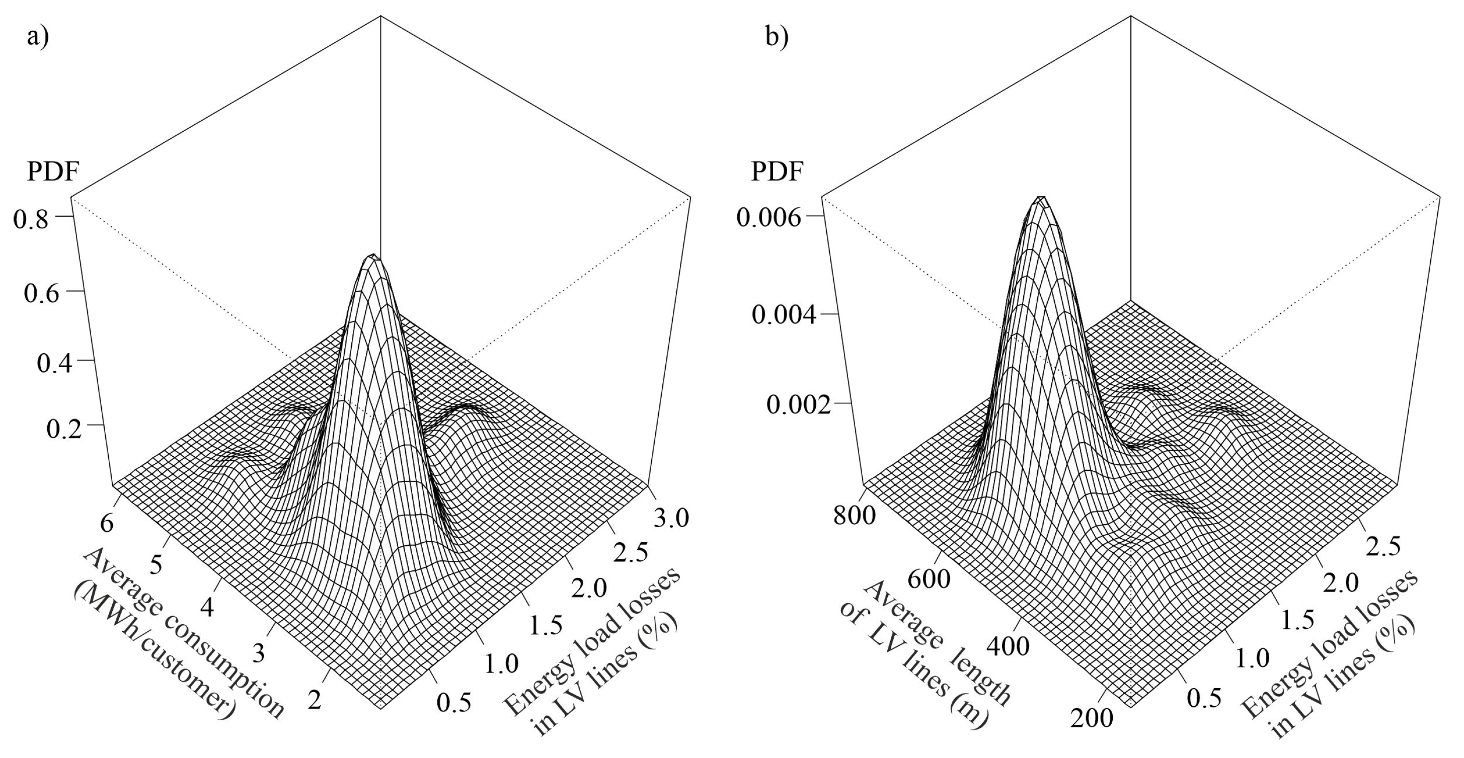
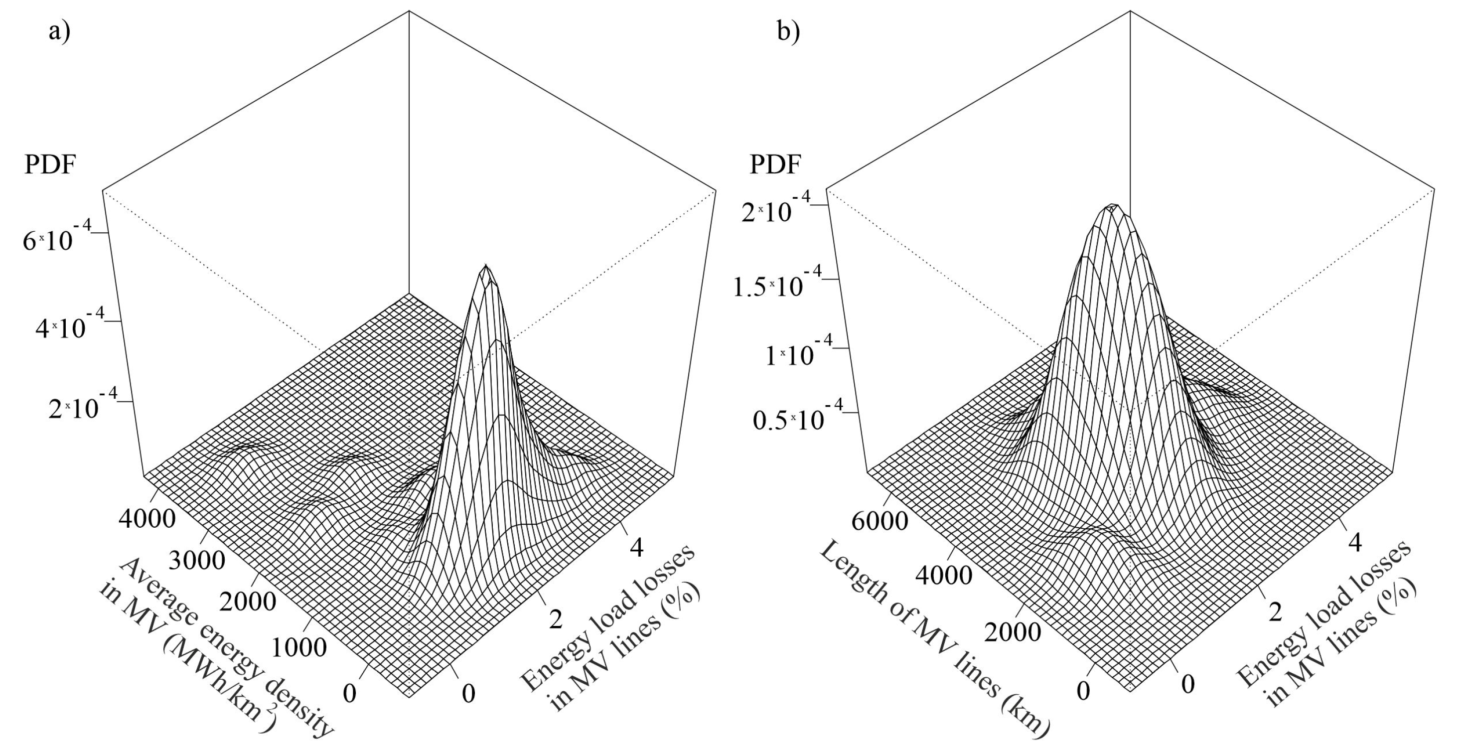
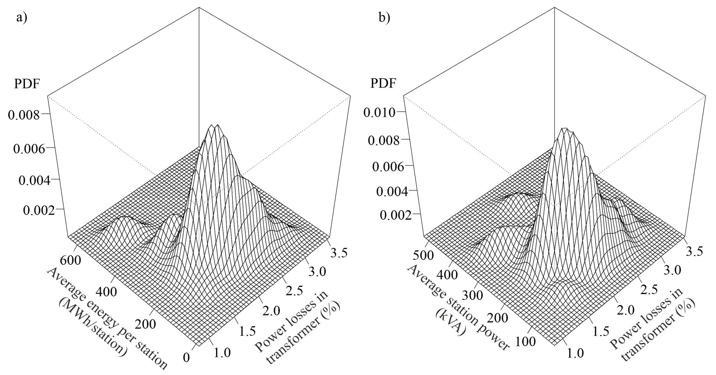
3.1. Network Loss Analysis

In order to analyse the operation of electricity distribution networks, data from 41 national distribution areas (accounting for over 40% of the territory of Poland) were collected and processed. The data concerned energy introduced and sold from the LV and MV grids, balance losses occurring in these grids and technical parameters such as area, length of lines making up the LV and MV grids, in addition to the number and power of MV/LV transformers. Measurement of distribution areas provides information on balance losses in the 110 kV network and together in the LV as well as the MV. In order to determine the energy losses in individual network elements, it is necessary to calculate them.The STRATY (LOSSES) program [3] was used for this purpose. Among others, load losses in the LV and MV grid lines and losses in the MV/LV transformers were calculated. Using kernel estimators, studies were carried out to determine which distribution areas have high energy losses, and then to assess what is causing it.

Figure 1 presents the analysis of energy losses for low voltage networks using two-dimensional estimation of the probability density function of the analysed variables with the normal kernel. The variables in Figure 1a relate to the average energy consumption by the recipient supplied from the low voltage network and the percentage of load losses occurring in the lines of this network. Figure 1b shows the average length of the low voltage line in relation to the percentage of load losses in the lines. All drawings in the article obtained using the ks library in the R environment [57].

Smoothing coefficients H have the values $\left[\begin{array}{cc}0.028898& 0\\ 0& 0.092538\end{array}\right]$ for the average energy consumption vs. the percentage of load losses occurring in the LV lines and $\left[\begin{array}{cc}0.026907& 0\\ 0& 1802.17\end{array}\right]$ for the average line length, respectively (Figure 1b). The graphs show a relatively high heterogeneity of the low voltage grid, much greater in the case of the average line length analysis than in the case of the average energy consumption by the consumer. The load energy losses in the LV lines are from 0.63% to 2.37%, the median is 1.05%; the average energy consumption of a single consumer supplied from the low voltage grid is from 2.28 to 5.05 MWh/consumer/year and the median is 3.07 MWh/consumer; the average length of the low-voltage line is from 305 m to 651 m; the median is 547 m. Some distribution areas have significantly different (higher or lower) energy losses from other areas. The conducted study showed that the lower energy losses resulted from much shorter network circuits, characteristic of cable networks. The higher load energy losses were the result of long low voltage grid circuits. Long line circuits, even at low loads, can be a problem for distribution companies and investment efforts should be stepped up in these areas.

Figure 2 presents the two-dimensional PDF function of load energy losses in the medium-voltage network. Figure 2a shows the energy density and percentage load losses occurring in the lines of the medium voltage network, Figure 2b shows the length of the medium-voltage lines and the percentage load losses occurring in these lines.

Smoothing coefficients H have the values $\left[\begin{array}{cc}0.133551& 0\\ 0& 45535.7\end{array}\right]$ for the energy density and percentage load losses and $\left[\begin{array}{cc}0.125045& 0\\ 0& 213742\end{array}\right]$ for average line length and percentage load losses occurring in the MV lines, respectively. The diagrams show the high heterogeneity of the medium-voltage network. The load energy losses in the MV lines range from 0.25% to 4.12%, the median is 1.90%; the energy density in the medium voltage network ranges from approx. 80 to approx. 7000 MWh/km², the median is 232 MWh/km²; the length of the medium-voltage lines ranges from 786 km to 4697 km, the median is 2732 km. Significantly lower values of the load energy losses are due to the high energy density. The high-load energy losses are associated with long strings of medium-voltage lines. The low energy losses occur with high energy density, which is characteristic of cable networks. Further analysis should be carried out in these areas in order to more accurately determine the cause of the high energy losses. If the scope of the collected data allows, the analysis should be carried out separately for cable lines and overhead lines.

Figure 3 shows the results of the analysis of losses occurring in MV/LV transformers. Figure 3a shows the KDE for the energy fed into the grid by the substation and the percentage losses of MV/LV transformers, while Figure 3b shows the average power of the substation in relation to the percentage losses of MV/LV transformers.

Smoothing coefficients H have the values $\left[\begin{array}{cc}0.023652& 0\\ 0& 811.289\end{array}\right]$ for the energy output from MV/LV substations and percentage losses in MV/LV transformers. For Figure 3b, this coefficient was $\left[\begin{array}{cc}0.022917& 0\\ 0& 617.823\end{array}\right]$. The energy losses in the transformers range from 1.37% to 3.0%, median 1.96%; the average power of the transformers ranges from 95 kVA to 424 kVA; median 147 kVA, the energy transferred annually by the transformer ranges from 90 MWh to 500 MWh, the median is 167 MWh.

The graphs show a large heterogeneity of losses in the MV/LV transformers. It may result from several reasons: (1) load losses depend on the transformer load factor; the lower the load, the lower the losses, but the technical losses in transformers (voltage and load) are higher, (2) transformers of different classes operate in networks; thus, the transformer class determines the size of losses. Further analysis of the outliers should be carried out to ascertain the cause of the too high energy losses.

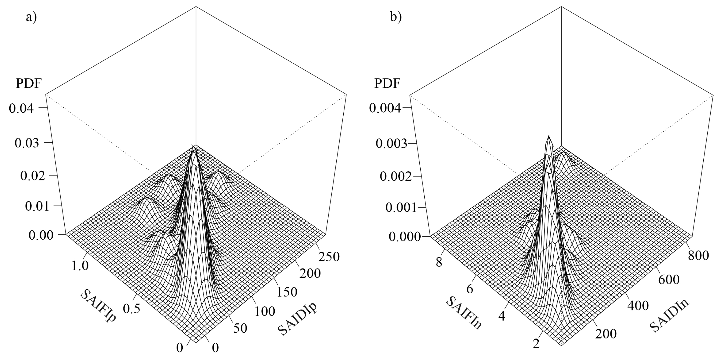
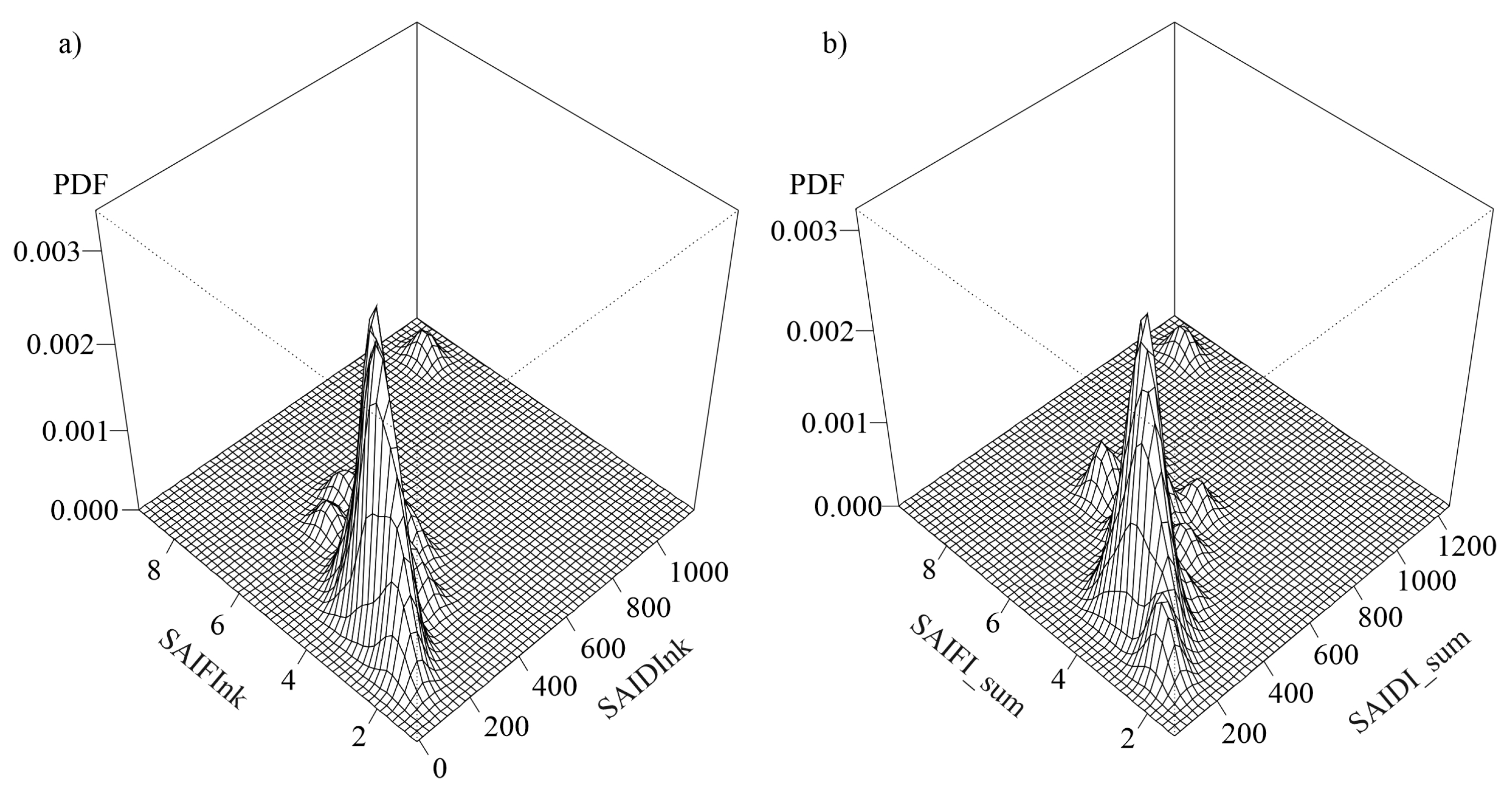
3.2. Reliability Analysis

In the second part of the study, the operation of 41 distribution areas was analysed, the same for which the network loss analysis was carried out, in terms of its operational reliability. The SAIDI (System Average Outage Duration Index) and SAIFI (System Average Outage Frequency Index) indicators are commonly used in the global reliability analysis. SAIDI is an indicator of the average system duration of a long and very long outage in electricity supply, expressed in minutes per customer per year, being the sum of the products of its duration and the number of customers exposed to the effects of this outage during the year, divided by the total number of customers served. Similarly, SAIFI refers to the average system frequency of long and very long outages in electricity supply, which is the number of all these outages during the year, divided by the total number of customers served.

The SAIDI and SAIFI indicators are determined separately for scheduled and unplanned outages. In Poland, during calculations, catastrophic outages, i.e., outages lasting longer than 24 h, should be analysed separately. SAIDI and SAIFI do not include short outages lasting less than 3 min.

Figure 4a presents the two-dimensional PDF of the distribution of the SAIFI for scheduled outages (SAIFIp) and SAIDI for scheduled outages (SAIDIp) indicators, while Figure 4b presents the SAIFI for unplanned outages (SAIFIn) as well as SAIDI for unplanned outages (SAIDIn) indicators.

Smoothing coefficients H have the values $\left[\begin{array}{cc}149.239& 0\\ 0& 0.002879\end{array}\right]$ for scheduled outages (SAIFIp, SAIDIp) and $\left[\begin{array}{cc}610.924& 0\\ 0& 0.075972\end{array}\right]$ for unplanned outages (SAIFIn, SAIDIn), respectively. There is a large scatter in the values of both planned and unplanned outages. The SAIFIp values are from 0.153 to 1.026, the median is 0.4223; SAIDIp is from 26.45 to 229.80, the medianis 78.96. These dispersions are related to different policies for carrying out planned works, implemented by individual regions. For unplanned outages, SAIFIn is from 1.998 to 7.962 and SAIDIn from 106.6 to 755.0. The medians are 3.653 and 214.2, respectively. It should be noted that in one of the analysed areas there were above-average, unfavourable weather conditions, which were reflected in the SAIFIn and SAIDIn values.

Figure 5a presents the analysis of the distribution of the average system index for unplanned long and very long outages with catastrophic outages, respectively for the duration (SAIDInk) and their frequency (SAIFInk) of the analysed 41 regions. Similarly, Figure 5b presents the distributions for the sum of the times of all planned and unplanned outages together with catastrophic (SAIFI_sum, SAIDI_sum).

H for unplanned and catastrophic outages (SAIFInk, SAIDInk) and for the sum of all outages (SAIFI_sum, SAIDI_sum) have the same values $\left[\begin{array}{cc}992.771& 0\\ 0& 0.082053\end{array}\right]$. This proves the fact that the value of planned outages has a slight impact on the total value of planned and unplanned outages. The SAIFInk values are 1.99 to 8.08, the median is 3.66; while SAIDInk is from 107.2 to 1056.8, the median is 219.2. For the sum of planned and unplanned outages together with catastrophic events, SAIFI_sum ranges from 2.31 to 8.49, and SAID_sum from 142.5 to 1138.7. The medians are 3.98 and 300.4, respectively. The outliers refer to the area with unfavourable weather conditions.

4. Conclusions

The analyses carried out in this study allow for the following conclusions:

• The non-parametric approach is much more flexible than the parametric approach. The estimation of the density function of the analysed random variables using KDE provides a productive tool for assessing the operation of the distribution system.
• The presented analysis of the data on the operation of distribution networks allows areas to be found for which energy losses or reliability levels are outliers in relation to other regions, and enables distribution companies to optimally invest their funds in the distribution network. This method was used in the energy audit for one of the Distribution System Operators.
• The analysis of the operation of national distribution networks shows the need for large investments in selected parts of the network. On the basis of the conducted study, it is possible to precisely indicate which areas should be modernised in the first place.
• Indicating outliers allows you to narrow down the area for which, having more detailed data, such as e.g., grid diagrams, energy fed into a given line or transformer, it is possible to conduct an in-depth analysis and determine which lines or transformers require modernisation.
• The main reasons for the differences in the levels of network reliability in individual areas include: various share of cable lines in the network, the renovation policy implemented or the strategy of managing failure and post-emergency works.
• It should be noted that distribution companies are currently facing new challenges related to adapting the distribution network to integration with dynamically installed distributed energy sources.

References

1. Wang, S.; Yang, J.; Gao, K.; Li, J. Energy Efficiency Analysis of Power System Based on Optimization of Peak Supply and Demand Regulation. In Proceedings of the International Conference on Smart Grid and Electrical Automation (ICSGEA), Changsha, China, 9–10 June 2018; pp. 104–107. [Google Scholar]
2. Gawlak, A. Profitability Analysis of Investment Projects in Distribution Networks. Prz. Elektrotechniczny 2019, 95, 13–16. [Google Scholar] [CrossRef]
3. Gawlak, A. Directions of investment and the loss of electricity in the distribution network. Prz. Elektrotechniczny 2017, 93, 40–43. (In Polish) [Google Scholar]
4. Girbau-Llistuella, F.; Díaz-González, F.; Sumper, A.; Gallart-Fernández, R.; Heredero-Peris, D. Smart Grid Architecture for Rural Distribution Networks: Application to a Spanish Pilot Network. Energies 2018, 11, 844. [Google Scholar] [CrossRef] [Green Version]
5. Barone, G.; Brusco, G.; Burgio, A.; Menniti, D.; Pinnarelli, A.; Motta, M.; Sorrentino, N.; Vizza, P. A Real-Life Application of a Smart User Network. Energies 2018, 11, 3504. [Google Scholar] [CrossRef] [Green Version]
6. Li, H.; Cui, H.; Li, C. Distribution Network Power Loss Analysis Considering Uncertainties in Distributed Generations. Sustainability 2019, 11, 1311. [Google Scholar] [CrossRef] [Green Version]
7. Kumar, S.; Sarita, K.; Vardhan, A.S.S.; Elavarasan, R.M.; Saket, R.K.; Das, N. Reliability Assessment of Wind-Solar PV Integrated Distribution System Using Electrical Loss Minimization Technique. Energies 2020, 13, 5631. [Google Scholar] [CrossRef]
8. Shrestha, T.K.; Karki, R. Utilizing Energy Storage for Operational Adequacy of Wind-Integrated Bulk Power Systems. Appl. Sci. 2020, 10, 5964. [Google Scholar] [CrossRef]
9. Gawlak, A.; Kornatka, M.; Kolcun, M.; Čonka, Z. Active and Reactive Power Losses in Distribution Transformers. Acta Polytech. Hung. 2020, 17, 161–174. [Google Scholar]
10. Atanasovski, M.; Taleski, R. Energy summation method for loss allocation in radial distribution networks with DG. IEEE Trans. Power Syst. 2012, 27, 1433–1440. [Google Scholar] [CrossRef]
11. Hoffman, R. Practical State Estimation for Electric Distribution Networks. In Proceedings of the IEEE PES Power Systems Conference and Exposition, Atlanta, GA, USA, 29 October–1 November 2006; pp. 510–517. [Google Scholar] [CrossRef]
12. Naka, S.; Genji, T.; Yura, T.; Fukuyama, Y. Practical distribution state estimation using hybrid particle swarm optimization. In Proceedings of the IEEE Power Engineering Society Winter Meeting, Columbus, OH, USA, 28 January–1 February 2001; Volume 2, pp. 815–820. [Google Scholar] [CrossRef] [Green Version]
13. Sarić, A.T.; Ćirić, R.M. Integrated fuzzy state estimation and load flow analysis in distribution networks. Trans. Power Deliv. 2003, 18, 571–578. [Google Scholar] [CrossRef]
14. Wan, J.; Miu, K.N. Weighted least squares methods for load estimation in distribution networks. IEEE Trans. Power Syst. 2003, 18, 1338–1345. [Google Scholar] [CrossRef]
15. Baran, M.E.; Freeman, A.A.; Hanson, F.; Ayers, V. Load estimation for load monitoring at distribution substations. IEEE Trans. Power Syst. 2005, 20, 164–170. [Google Scholar] [CrossRef]
16. Hasanpor Divsheli, P.; Ghadiri, H.; Hesaminia, A.H.; Amini, B. A novel approach for meter placement for load estimation in radial distribution networks. In Proceedings of the Third International Conference on Electric Utility Deregulation and Restructuring and Power Technologies, Nanjing, China, 6–9 April 2008; pp. 1576–1579. [Google Scholar] [CrossRef]
17. Baghaee, H.R.; Mirsalim, M.; Gharehpetian, G.B.; Talebi, H.A. Generalized three phase robust load-flow for radial and meshed power systems with and without uncertainty in energy resources using dynamic radial basis functions neural networks. J. Clean. Prod. 2018, 174, 96–113. [Google Scholar] [CrossRef]
18. Baghaee, H.R.; Mirsalim, M.; Gharehpetan, G.B.; Talebi, H.A. Nonlinear load sharing and voltage compensation of microgrids based on harmonic power-flow calculations using radial basis function neural networks. IEEE Syst. J. 2018, 12, 2749–2759. [Google Scholar] [CrossRef]
19. Jagtap, K.M.; Khatod, D.K. Loss allocation in radial distribution networks with various distributed generation and load models. Int. J. Electr. Power Energy Syst. 2016, 75, 173–186. [Google Scholar] [CrossRef]
20. Baghaee, H.R.; Mirsalim, M.; Gharehpetian, G.B. Performance Improvement of Multi-DER Microgrid for Small- and Large-Signal Disturbances and Nonlinear Loads: Novel Complementary Control Loop and Fuzzy Controller in a Hierarchical Droop-Based Control Scheme. IEEE Syst. J. 2018, 12, 444–451. [Google Scholar] [CrossRef]
21. Wu, J.; Yu, Y. CBR-based load estimation for distribution networks. In Proceedings of the MELECON 2006-IEEE Mediterranean Electrotechnical Conference, Malaga, Spain, 16–19 May 2006; pp. 952–955. [Google Scholar] [CrossRef]
22. Falcão, D.M.; Henriques, H.O. Load estimation in radial distribution systems using neural networks and fuzzy set techniques. In Proceedings of the IEEE Power Engineering Society Summer Meeting, Conference Proceedings, Vancouver, BC, Canada, 15–19 July 2001; Volume 2, pp. 1002–1006. [Google Scholar] [CrossRef]
23. Wang, S.; Dong, P.; Tian, Y. A Novel Method of Statistical Line Loss Estimation for Distribution Feeders Based on Feeder Cluster and Modified XGBoost. Energies 2017, 10, 2067. [Google Scholar] [CrossRef] [Green Version]
24. Iqteit, N.A.; Arsoy, A.; Çakir, B. A Simple Method to Estimate Power Losses in Distribution Networks. In Proceedings of the 10th International Conference on Electrical and Electronics Engineering (ELECO), Bursa, Turkey, 30 November–2 December 2017; pp. 135–140. [Google Scholar]
25. Mikic, O.M. Variance-based energy loss computation in low voltage distribution networks. IEEE Trans. Power Syst. 2017, 22, 179–187. [Google Scholar] [CrossRef]
26. Celli, G.; Natale, N.; Pilo, F.; Pisano, G.; Bignucolo, F.; Coppo, M.; Savio, A.; Turri, R.; Cerretti, A. Containment of power losses in LV networks with high penetration of distributed generation. In Proceedings of the 24th International Conference and Exhibition on Electricity Distribution (CIRED), Glasgow, UK, 12–15 June 2017. [Google Scholar] [CrossRef] [Green Version]
27. Szkutnik, J.; Gawlak, A. Optimalization-based method of dividing the network development costs. Electr. Eng. 2011, 93, 137–146. [Google Scholar] [CrossRef] [Green Version]
28. Billinton, R.; Li, W. Reliability Assessment of Electric Power Systems Using Monte Carlo Methods; Springer: New York, NY, USA, 1994. [Google Scholar]
29. Billinton, R.; Allan, R.N. Reliability Evaluation of Power System, 2nd ed.; Springer: New York, NY, USA, 1996. [Google Scholar]
30. Billinton, R. Canadian experience in the collection of transmission and distribution component unavailability data. In Proceedings of the International Conference on Probabilistic Methods Applied to Power Systems, Aimes, IA, USA, 12–16 September 2004; pp. 268–273. [Google Scholar]
31. Billinton, R.; Singh, G. Application of adverse, extreme adverse weather: Modelling in transmission, distribution system reliability evaluation. IEE Proc.-Gener. Transm. Distrib. 2006, 153, 115–120. [Google Scholar] [CrossRef]
32. Ding, Y.; Wang, S.; Goel, L.; Billinton, R.; Karki, R. Reliability assessment of restructured power systems using reliability network equivalent, pseudo-sequential simulation techniques. Electr. Power Syst. Res. 2007, 77, 1665–1671. [Google Scholar] [CrossRef]
33. Allan, R.N.; Billinton, R. Concepts of Power Systems Reliability Evaluation. Electr. Power Energy Syst. 1988, 10, 39–141. [Google Scholar] [CrossRef]
34. Allan, R.N.; Billinton, R. Power System Reliability and its Assessment. Part 1: Background and Generating Capacity. Power Eng. J. 1992, 6, 191–196. [Google Scholar] [CrossRef]
35. Allan, R.N.; Billinton, R. Power System Reliability and its Assessment. Part 2: Composite Generation and Transmission Systems. Power Eng. J. 1992, 6, 291–297. [Google Scholar] [CrossRef]
36. Allan, R.N.; Billinton, R. Power System Reliability and its Assessment. Part 3: Distribution Systems and Economic Considerations. Power Eng. J. 1993, 7, 185–192. [Google Scholar] [CrossRef]
37. Paska, J.; Marchel, P. Bezpieczeństwo Elektroenergetyczne i Niezawodność Zasilania Energią Elektryczną (Electricity Security and Reliability of Electricity Supply); Oficyna Wydawnicza Politechniki Warszawskiej: Warsaw, Poland, 2021. (In Polish) [Google Scholar]
38. Zio, E. Reliability engineering: Old problems and new challenges. Reliab. Eng. Syst. Saf. 2009, 94, 125–141. [Google Scholar] [CrossRef] [Green Version]
39. Pombo, A.V.; Murta-Pina, J.; Pires, F. Multiobjective planning of distribution networks incorporating switches and protective devices using a memetic optimization. Reliab. Eng. Syst. Saf. 2015, 136, 101–108. [Google Scholar] [CrossRef]
40. Ziari, I.; Ledwich, G.; Ghosh, A. Optimal integrated planning of MV-LV distribution systems using DPSO. Electr. Power Syst. Res. 2011, 81, 1905–1914. [Google Scholar] [CrossRef]
41. Hemdan, N.; Deppe, B.; Pielke, M.; Kurrat, M.; Schmedes, T.; Wieben, E. Optimal reconfiguration of radial MV networks with load profiles in the presence of renewable energy based decentralized generation. Electr. Power Syst. Res. 2014, 116, 355–366. [Google Scholar] [CrossRef]
42. Bai, X.; Asgarpoor, S. Fuzzy-based approaches to substation reliability evaluation. Electr. Power Syst. Res. 2004, 69, 197–204. [Google Scholar] [CrossRef]
43. Polansky, A. A smooth nonparametric approach to process capability. Qual. Reliab. Eng. 1998, 14, 43–48. [Google Scholar] [CrossRef]
44. Saleh, J.; Marais, K. Highlights from the early (and pre-) history of reliability engineering. Reliab. Eng. Syst. Saf. 2006, 91, 249–256. [Google Scholar] [CrossRef]
45. Qualitative Regulation in 2018–2025 for Distribution System Operators (Who Separated Their Activities as of 1 July 2007); Energy Regulatory Office: Warsaw, Poland, 2018. (In Polish)
46. IEEE Guide for Electric Power Distribution Reliability Indices. In IEEE Std 1366-2012 (Revision of IEEE Std 1366-2003); IEEE: Piscataway Township, NJ, USA, 31 May 2012; pp. 1–43. [CrossRef]
47. Kornatka, M. The weighted kernel density estimation methods for analysing reliability of electricity supply. In Proceedings of the 17th International Scientific Conference on Electric Power Engineering (EPE), Prague, Czech Republic, 16–18 May 2016; pp. 1–4. [Google Scholar] [CrossRef]
48. Chacón, J.E.; Duong, T. Multivariate Kernel Smoothing and Its Applications, 1st ed.; Chapman and Hall/CRC: Boca Raton, FL, USA, 2018. [Google Scholar]
49. Silverman, B.W. Density Estimation for Statistics and Data Analysis; Chapman and Hall: London, UK; New York, NY, USA, 1986. [Google Scholar]
50. Duong, T. ks Kernel density estimation and kernel discriminant analysis in R. J. Stat. Softw. 2007, 21. [Google Scholar] [CrossRef] [Green Version]
51. Lotfi, M.; Javadi, M.; Osório, G.J.; Monteiro, C.; Catalão, J.P.S. A Novel Ensemble Algorithm for Solar Power Forecasting Based on Kernel Density Estimation. Energies 2020, 13, 216. [Google Scholar] [CrossRef] [Green Version]
52. Zhang, L.; Xie, L.; Han, Q.; Wang, Z.; Huang, C. Probability Density Forecasting of Wind Speed Based on Quantile Regression and Kernel Density Estimation. Energies 2020, 13, 6125. [Google Scholar] [CrossRef]
53. Chen, L.; Huang, X.; Zhang, H. Modeling the Charging Behaviors for Electric Vehicles Based on Ternary Symmetric Kernel Density Estimation. Energies 2020, 13, 1551. [Google Scholar] [CrossRef] [Green Version]
54. Ghorbanzadeh, M.; Koloushani, M.; Ulak, M.B.; Ozguven, E.E.; Jouneghani, R.A. Statistical and Spatial Analysis of Hurricane-induced Roadway Closures and Power Outages. Energies 2020, 13, 1098. [Google Scholar] [CrossRef] [Green Version]
55. Wang, J.; Zhang, C.; Ma, X.; Wang, Z.; Xu, Y.; Cattley, R. A Multivariate Statistics-Based Approach for Detecting Diesel Engine Faults with Weak Signatures. Energies 2020, 13, 873. [Google Scholar] [CrossRef] [Green Version]
56. Lin, Z.; Duan, D.; Yang, Q.; Hong, X.; Cheng, X.; Yang, L.; Cui, S. Data-Driven Fault Localization in Distribution Systems with Distributed Energy Resources. Energies 2020, 13, 275. [Google Scholar] [CrossRef] [Green Version]
57. R Evelopment Core Team © R: A Language and Environment for Statistical Computing. Available online: https://cran.r-project.org/ (accessed on 31 August 2021).
Figure 1. Two-dimensionaldensity function obtained by means of KDE function for: (a) average consumption and energy load losses in LV (b) average length of LV lines and energy load losses in LV.
Energies 14 06984 g001
Figure 2. Two-dimensional density function obtained by means of KDE function for: (a) average energy density in MV and energy load losses in MV lines, (b) length of MV lines and energy load losses in MV.
Energies 14 06984 g002
Figure 3. Two-dimensional density function obtained by means of KDE function for: (a) average energy per station and power losses in transformer MV/LV, (b) average station power and power losses in transformer MV/LV.
Energies 14 06984 g003
Figure 4. Two-dimensional density function obtained by means of KDE function for: (a) scheduled outages (SAIFIp, SAIDIp), (b) unplanned outages (SAIFIn, SAIDIn).
Energies 14 06984 g004
Figure 5. Two-dimensional density function obtained by means of KDE function for: (a) sum of unplanned outages and catastrophic outages (SAIFInk, SAIDInk), (b) sum of planned outages and unplanned outages and catastrophic events (SAIFI_sum, SAIDI_sum).
Energies 14 06984 g005