
Revisiting the Role of Fiscal Policy, Financial Development, and Foreign Direct Investment in Reducing Environmental Pollution during Globalization Mode: Evidence from Linear and Nonlinear Panel Data Approaches


Abstract
:1. Introduction
2. Literature Review
2.1. Nexus between Fiscal Policy and CO2 Emissions
2.2. Nexus between Financial Development and CO2 Emissions
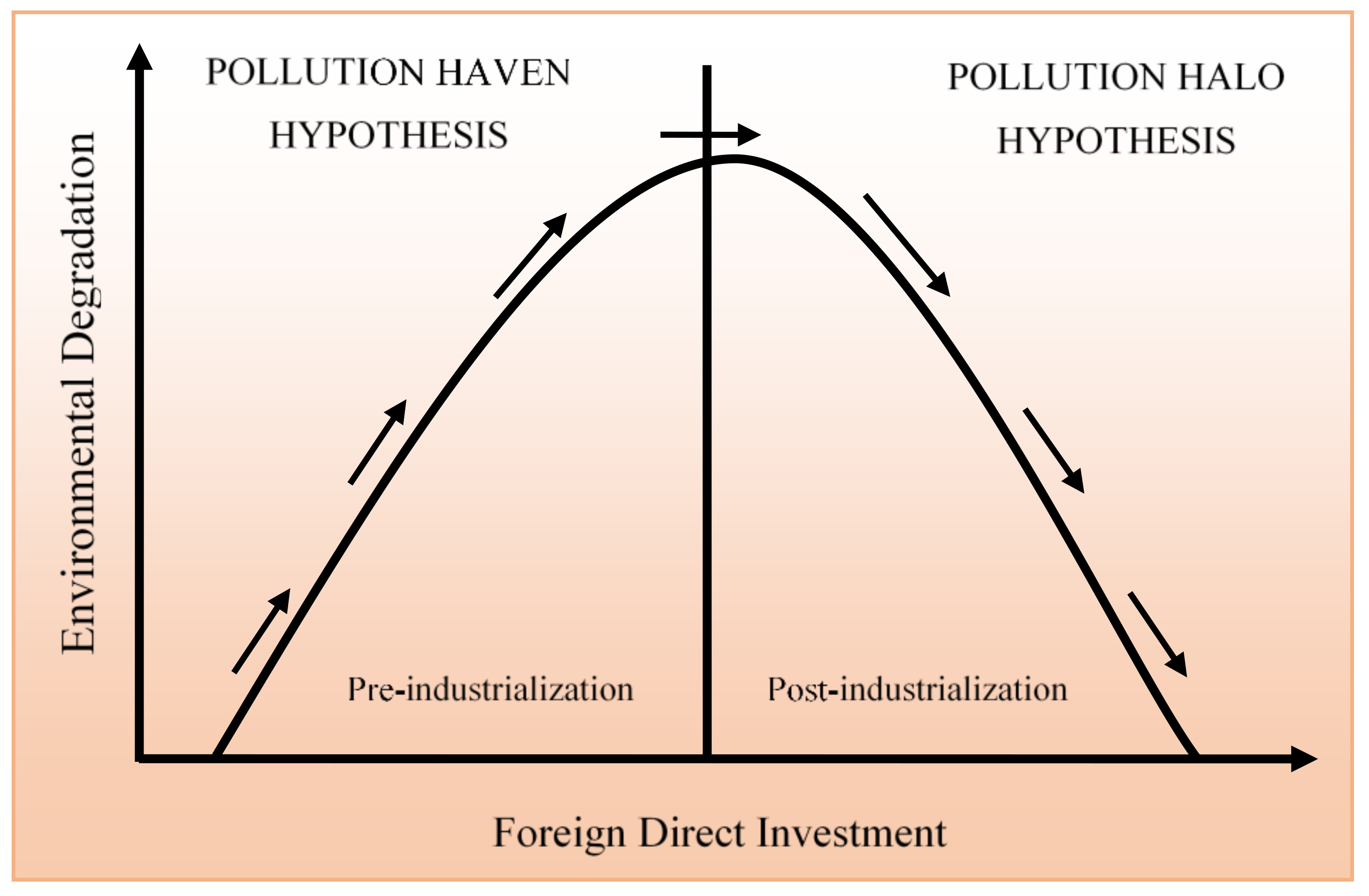
2.3. Nexus between Foreign Direct Investment and CO2 Emissions
2.4. Nexus between Trade Openness, Labour Force, and CO2 Emissions
2.5. Nexus between Urban Population, Gross Capital Formation, and CO2 Emissions
3. Empirical Strategy
3.1. Model and Data
3.2. Panel Unit Root Tests
3.3. Panel Cointegration Tests
3.4. Long-Run Elasticity Estimates (Linear)
3.4.1. Full Modified Ordinary Least Square (FMOLS)
3.4.2. Dynamic Ordinary Least Square (DOLS)
3.4.3. Autoregressive Distributive Lag Model (PMG/ARDL)
3.5. Panel Threshold Regression (Nonlinear)
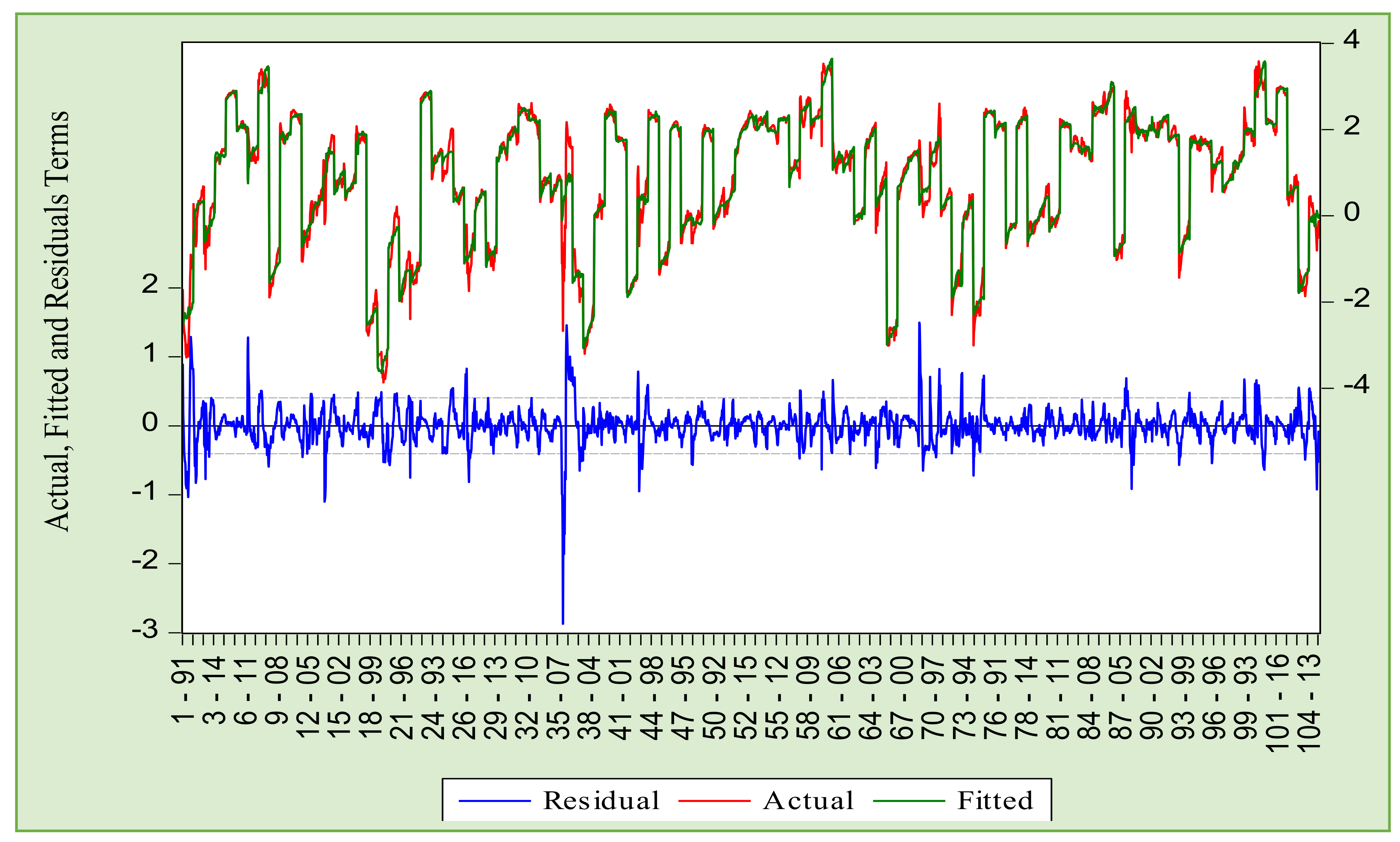
4. Results and Discussion
4.1. Results of Panel Unit Root Tests
4.2. Results of Panel Cointegration Tests
4.3. Results of Panel Long-Run Elasticity Estimates
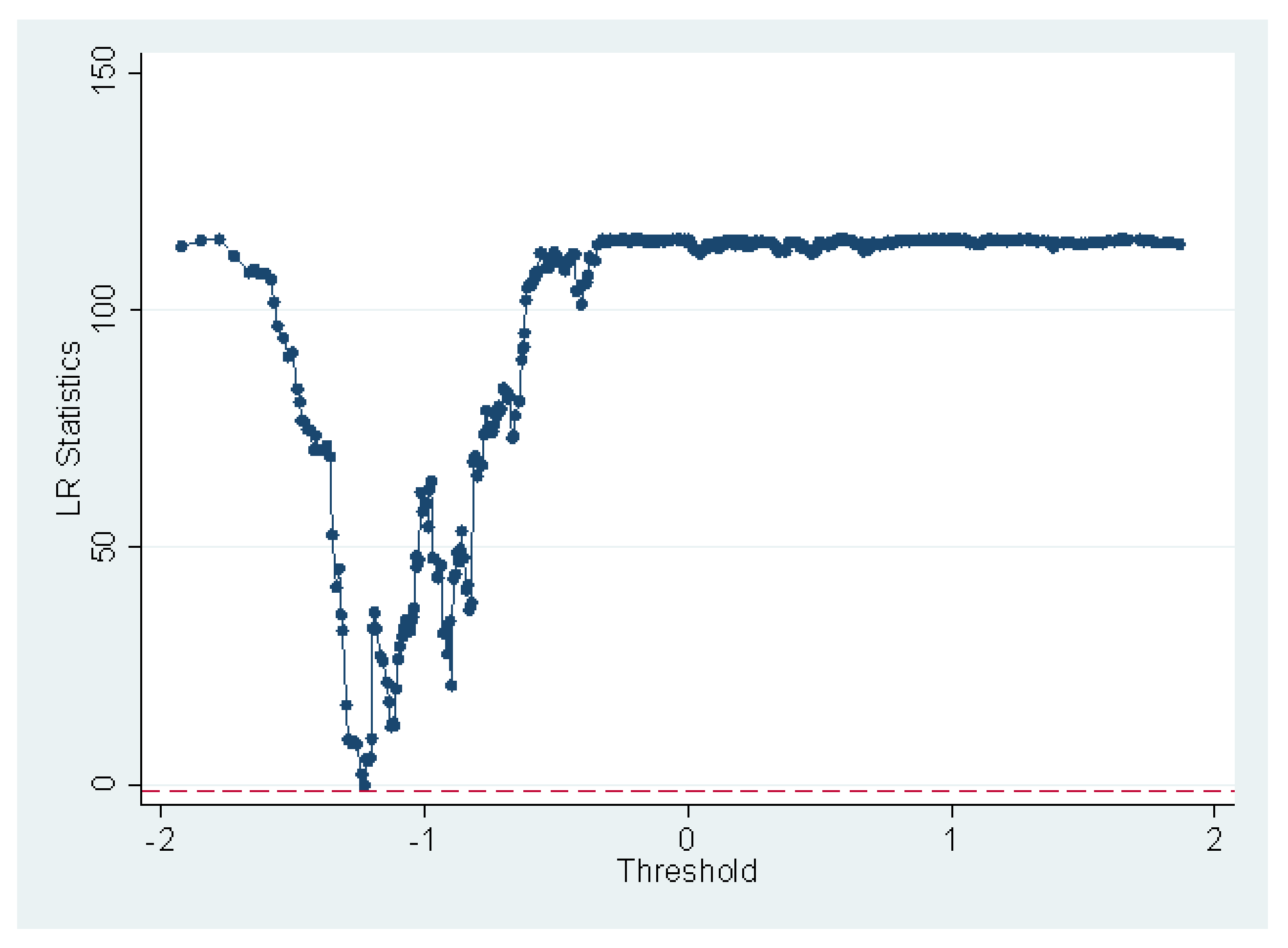
4.4. Identifying the Threshold Level
5. Conclusions and Policy Implications
Author Contributions
Funding
Institutional Review Board Statement
Informed Consent Statement
Data Availability Statement
Conflicts of Interest
Appendix A

| Afghanistan | Cameroon | Georgia | Lithuania | Portugal |
| Albania | Canada | Germany | Madagascar | Romania |
| Angola | Chile | Ghana | Malaysia | Russian Federation |
| Argentina | China | Greece | Maldives | Saudi Arabia |
| Australia | Colombia | Honduras | Mali | Singapore |
| Austria | Congo, Rep. | Hungary | Mauritius | Slovenia |
| Azerbaijan | Costa Rica | Iceland | Mexico | South Africa |
| Bahrain | Cote d’Ivoire | India | Moldova | Spain |
| Bangladesh | Croatia | Indonesia | Mongolia | Sri Lanka |
| Belarus | Cyprus | Iran, Islamic Rep. | Morocco | Sweden |
| Belgium | Czech Republic | Ireland | Myanmar | Switzerland |
| Bhutan | Denmark | Israel | Namibia | Thailand |
| Bolivia | Dominican Republic | Italy | Nepal | Tunisia |
| Bosnia and Herzegovina | Egypt, Arab Rep. | Japan | Netherlands | Turkey |
| Botswana | Equatorial Guinea | Jordan | New Zealand | Ukraine |
| Brazil | Estonia | Kazakhstan | Nicaragua | United Arab Emirates |
| Bulgaria | Ethiopia | Korea, Rep. | Norway | United Kingdom |
| Burkina Faso | Fiji | Kuwait | Paraguay | United States |
| Burundi | Finland | Latvia | Peru | Uruguay |
| Cape Verde | France | Lebanon | Philippines | Zambia |
| Cambodia | Gambia | Lesotho | Poland | Zimbabwe |
References
- Hafeez, M.; Yuan, C.; Yuan, Q.; Zhuo, Z.; Stromaier, D. A global prospective of environmental degradations: Economy and finance. Environ. Sci. Pollut. Res. 2019, 26, 25898–25915. [Google Scholar] [CrossRef] [PubMed]
- Burke, P. Fiscal Policies for Development and Climate Action. Bull. Indones. Econ. Stud. 2019, 55, 263–264. [Google Scholar] [CrossRef]
- Halkos, G.E.; Paizanos, E.A. The effect of government expenditure on the environment: An empirical investigation. Ecol. Econ. 2013, 91, 48–56. [Google Scholar] [CrossRef]
- López, R.; Galinato, G.I.; Islam, A. Fiscal spending and the environment: Theory and empirics. J. Environ. Econ. Manag. 2011, 62, 180–198. [Google Scholar] [CrossRef]
- Sarkodie, S.A.; Adams, S.; Owusu, P.A.; Leirvik, T.; Ozturk, I. Mitigating degradation and emissions in China: The role of environmental sustainability, human capital and renewable energy. Sci. Total Environ. 2020, 719, 137530. [Google Scholar] [CrossRef]
- Bolat, S.; Emirmahmutoglu, F.; Belke, M. The Dynamic Linkages of Budget Deficits and Current Account Deficits Nexus in EU Countries: Bootstrap Panel Granger Causality Test. Int. J. Econ. Perspect. 2014, 8, 16–26. [Google Scholar]
- Islam, A.M.; López, R.E. Government Spending and Air Pollution in the US. International Review of Environmental and Resource Economics. 2014. Available online: https://ageconsearch.umn.edu/record/144406/ (accessed on 19 March 2021).
- López, R.; Palacios, A. Why has Europe become environmentally cleaner? Decomposing the roles of fiscal, trade and environmental policies. Environ. Resour. Econ. 2014, 58, 91–108. [Google Scholar] [CrossRef]
- Farzanegan, M.R.; Feizi, M.; Gholipour, H.F. Globalization and the outbreak of COVID-19: An empirical analysis. J. Risk Financ. Manag. 2021, 14, 105. [Google Scholar]
- Blum, B.; Neumärker, B.K. Lessons from Globalization and the COVID-19 Pandemic for Economic, Environmental and Social Policy. World 2021, 2, 308–333. [Google Scholar] [CrossRef]
- Wang, X.; Yang, Q.; He, N. Research on the Influence of Environmental Regulation on Social Employment—An Empirical Analysis Based on the STR Model. Int. J. Environ. Res. Public Health 2020, 17, 622. [Google Scholar] [CrossRef] [Green Version]
- Zarsky, L. Havens, halos and spaghetti: Untangling the evidence about foreign direct investment and the environment. Foreign Direct Invest. Environ. 1999, 13, 47–74. [Google Scholar]
- Bakirtas, I.; Cetin, M.A. Revisiting the environmental Kuznets curve and pollution haven hypotheses: MIKTA sample. Environ. Sci. Pollut. Res. 2017, 24, 18273–18283. [Google Scholar] [CrossRef]
- Usman, M.; Kousar, R.; Yaseen, M.R.; Makhdum, M.S.A. An empirical nexus between economic growth, energy utilization, trade policy, and ecological footprint: A continent-wise comparison in upper-middle-income countries. Environ. Sci. Pollut. Res. 2020, 27, 38995–39018. [Google Scholar] [CrossRef]
- Ike, G.N.; Usman, O.; Sarkodie, S.A. Fiscal policy and CO2 emissions from heterogeneous fuel sources in Thailand: Evidence from multiple structural breaks cointegration test. Sci. Total Environ. 2020, 702, 134711. [Google Scholar] [CrossRef]
- Chishti, M.Z.; Ahmad, M.; Rehman, A.; Khan, M.K. Mitigations pathways towards sustainable development: Assessing the influence of fiscal and monetary policies on carbon emissions in BRICS economies. J. Clean. Prod. 2021, 292, 126035. [Google Scholar] [CrossRef]
- Ullah, S.; Ozturk, I.; Sohail, S. The asymmetric effects of fiscal and monetary policy instruments on Pakistan’s environmental pollution. Environ. Sci. Pollut. Res. 2021, 28, 7450–7461. [Google Scholar] [CrossRef]
- Chan, Y.T. Are macroeconomic policies better in curbing air pollution than environmental policies? A DSGE approach with carbon-dependent fiscal and monetary policies. Energy Policy 2020, 141, 111454. [Google Scholar] [CrossRef]
- Jain, V.; Purnomo, E.P.; Islam, M.M.; Mughal, N.; Guerrero, J.W.G.; Ullah, S. Controlling environmental pollution: Dynamic role of fiscal decentralization in CO2 emission in Asian economies. Environ. Sci. Pollut. Res. 2021, 134. [Google Scholar] [CrossRef]
- Khan, Z.; Ali, S.; Dong, K.; Li, R.Y.M. How does fiscal decentralization affect CO2 emissions? The roles of institutions and human capital. Energy Econ. 2021, 94, 105060. [Google Scholar] [CrossRef]
- Cheng, S.; Fan, W.; Chen, J.; Meng, F.; Liu, G.; Song, M.; Yang, Z. The impact of fiscal decentralization on CO2 emissions in China. Energy 2020, 192, 116685. [Google Scholar] [CrossRef]
- Langarita, R.; Cazcarro, I.; Sánchez-Chóliz, J.; Sarasa, C. The role of fiscal measures in promoting renewable electricity in Spain. Energy Convers. Manag. 2021, 244, 114480. [Google Scholar] [CrossRef]
- Tufail, M.; Song, L.; Adebayo, T.S.; Kirikkaleli, D.; Khan, S. Do fiscal decentralization and natural resources rent curb carbon emissions? Evidence from developed countries. Environ. Sci. Pollut. Res. 2021, 28, 49179–49190. [Google Scholar] [CrossRef]
- Lv, Z.; Li, S. How financial development affects CO2 emissions: A spatial econometric analysis. J. Environ. Manag. 2021, 277, 111397. [Google Scholar] [CrossRef]
- Shen, Y.; Su, Z.W.; Malik, M.Y.; Umar, M.; Khan, Z.; Khan, M. Does green investment, financial development and natural resources rent limit carbon emissions? A provincial panel analysis of China. Sci. Total Environ. 2021, 755, 142538. [Google Scholar] [CrossRef]
- Yang, B.; Jahanger, A.; Ali, M. Remittance inflows affect the ecological footprint in BICS countries: Do technological innovation and financial development matter? Environ. Sci. Pollut. Res. 2021, 28, 23482–23500. [Google Scholar] [CrossRef]
- Usman, M.; Makhdum, M.S.A.; Kousar, R. Does financial inclusion, renewable and non-renewable energy utilization accelerate ecological footprints and economic growth? Fresh evidence from 15 highest emitting countries. Sustain. Cities Soc. 2020, 65, 102590. [Google Scholar] [CrossRef]
- Usman, M.; Anwar, S.; Yaseen, M.R.; Makhdum, M.S.A.; Kousar, R.; Jahanger, A. Unveiling the dynamic relationship between agriculture value addition, energy utilization, tourism and environmental degradation in South Asia. J. Public Aff. 2021, e2712. [Google Scholar] [CrossRef]
- Al-Mulali, U.; Ozturk, I.; Lean, H.H. The influence of economic growth, urbanization, trade openness, financial development, and renewable energy on pollution in Europe. Nat. Hazards 2015, 79, 621–644. [Google Scholar] [CrossRef]
- Shahbaz, M.; Shahzad, S.J.H.; Ahmad, N.; Alam, S. Financial development and environmental quality: The way forward. Energy Policy 2016, 98, 353–364. [Google Scholar] [CrossRef] [Green Version]
- Bekhet, H.A.; Matar, A.; Yasmin, T. CO2 emissions, energy consumption, economic growth, and financial development in GCC countries: Dynamic simultaneous equation models. Renew. Sustain. Energy Rev. 2017, 70, 117–132. [Google Scholar] [CrossRef]
- Cetin, M.; Ecevit, E.; Yucel, A.G. The impact of economic growth, energy consumption, trade openness, and financial development on carbon emissions: Empirical evidence from Turkey. Environ. Sci. Pollut. Res. 2018, 25, 36589–36603. [Google Scholar] [CrossRef] [PubMed]
- Zafar, M.W.; Saud, S.; Hou, F. The impact of globalization and financial development on environmental quality: Evidence from selected countries in the Organization for Economic Co-operation and Development (OECD). Environ. Sci. Pollut. Res. 2019, 26, 13246–13262. [Google Scholar] [CrossRef] [PubMed]
- Dogan, E.; Seker, F. The influence of real output, renewable and non-renewable energy, trade and financial development on carbon emissions in the top renewable energy countries. Renew. Sustain. Energy Rev. 2016, 60, 1074–1085. [Google Scholar] [CrossRef]
- Zaidi, S.A.H.; Zafar, M.W.; Shahbaz, M.; Hou, F. Dynamic linkages between globalization, financial development and carbon emissions: Evidence from Asia Pacific Economic Cooperation countries. J. Clean. Prod. 2019, 228, 533–543. [Google Scholar] [CrossRef]
- Usman, M.; Hammar, N. Dynamic relationship between technological innovations, financial development, renewable energy, and ecological footprint: Fresh insights based on the STIRPAT model for Asia Pacific Economic Cooperation countries. Environ. Sci. Pollut. Res. 2021, 28, 15519–15536. [Google Scholar] [CrossRef]
- Nadeem, A.M.; Ali, T.; Khan, M.T.I.; Guo, Z. Relationship between inward FDI and environmental degradation for Pakistan: An exploration of pollution haven hypothesis through ARDL approach. Environ. Sci. Pollut. Res. 2020, 27, 15407–15425. [Google Scholar] [CrossRef]
- Yilanci, V.; Bozoklu, S.; Gorus, M.S. Are BRICS countries pollution havens? Evidence from a bootstrap ARDL bounds testing approach with a Fourier function. Sustain. Cities Soc. 2020, 55, 102035. [Google Scholar] [CrossRef]
- Balsalobre-Lorente, D.; Gokmenoglu, K.K.; Taspinar, N.; Cantos-Cantos, J.M. An approach to the pollution haven and pollution halo hypotheses in MINT countries. Environ. Sci. Pollut. Res. 2019, 26, 23010–23026. [Google Scholar] [CrossRef]
- Rana, R.; Sharma, M. Dynamic causality testing for EKC hypothesis, pollution haven hypothesis and international trade in India. J. Int. Trade Econ. Dev. 2019, 28, 348–364. [Google Scholar] [CrossRef]
- Khan, A.; Chenggang, Y.; Hussain, J.; Bano, S. Does energy consumption, financial development, and investment contribute to ecological footprints in BRI regions? Environ. Sci. Pollut. Res. 2019, 26, 36952–36966. [Google Scholar] [CrossRef]
- Ali, S.; Dogan, E.; Chen, F.; Khan, Z. International trade and environmental performance in top ten-emitters countries: The role of eco-innovation and renewable energy consumption. Sustain. Dev. 2021, 29, 378–387. [Google Scholar] [CrossRef]
- Nathaniel, S.P.; Murshed, M.; Bassim, M. The nexus between economic growth, energy use, international trade and ecological footprints: The role of environmental regulations in N11 countries. Energy Ecol. Environ. 2021, 6, 496–512. [Google Scholar] [CrossRef]
- Usman, M.; Jahanger, A. Heterogeneous effects of remittances and institutional quality in reducing environmental deficit in the presence of EKC hypothesis: A global study with the application of panel quantile regression. Environ. Sci. Pollut. Res. 2021. [Google Scholar]
- Rehman, A.; Radulescu, M.; Ma, H.; Dagar, V.; Hussain, I.; Khan, M.K. The Impact of Globalization, Energy Use, and Trade on Ecological Footprint in Pakistan: Does Environmental Sustainability Exist? Energies 2021, 14, 5234. [Google Scholar] [CrossRef]
- Lasisi, T.T.; Alola, A.A.; Eluwole, K.K.; Ozturen, A.; Alola, U.V. The environmental sustainability effects of income, labour force, and tourism development in OECD countries. Environ. Sci. Pollut. Res. 2020, 27, 21231–21242. [Google Scholar] [CrossRef]
- Qi, Y.; Xu, Z. Research on China’s Regional Economic Linkages: Based on the Analyses of Carbon Emission Transfers and Labor Mobility. Chin. J. Urban. Environ. Stud. 2019, 7, 1950002. [Google Scholar] [CrossRef]
- Anwar, A.; Younis, M.; Ullah, I. Impact of urbanization and economic growth on CO2 emission: A case of for east Asian countries. Int. J. Environ. Res. Public Health 2020, 17, 2531. [Google Scholar] [CrossRef] [Green Version]
- Abbasi, K.R.; Shahbaz, M.; Jiao, Z.; Tufail, M. How energy consumption, industrial growth, urbanization, and CO2 emissions affect economic growth in Pakistan? A novel dynamic ARDL simulations approach. Energy 2021, 221, 119793. [Google Scholar] [CrossRef]
- Rahman, Z.U.; Ahmad, M. Modeling the relationship between gross capital formation and CO2 (a) symmetrically in the case of Pakistan: An empirical analysis through NARDL approach. Environ. Sci. Pollut. Res. 2019, 26, 8111–8124. [Google Scholar] [CrossRef]
- Bekhet, H.A.; Yasmin, T.; Al-Smadi, R.W. Dynamic linkages among financial development, economic growth, energy consumption, CO2 emissions and gross fixed capital formation patterns in Malaysia. Int. J. Bus. Glob. 2017, 18, 493–523. [Google Scholar] [CrossRef]
- Hakimi, A.; Hamdi, H. Environmental effects of trade openness: What role do institutions have? J. Environ. Econ. Policy 2020, 9, 36–56. [Google Scholar] [CrossRef]
- Usman, M.; Yaseen, M.R.; Kousar, R.; Makhdum, M.S.A. Modeling financial development, tourism, energy consumption, and environmental quality: Is there any discrepancy between developing and developed countries. Environ. Sci. Pollut. Res. 2021. [Google Scholar] [CrossRef]
- Manning, W.G. The logged dependent variable, heteroscedasticity, and the retransformation problem. J. Health Econ. 1998, 17, 283–295. [Google Scholar] [CrossRef]
- World Bank. World Bank Database. 2020. Available online: https://databank.worldbank.org/data/source/world-development-indicators (accessed on 20 August 2021).
- Gygli, S.; Haelg, F.; Potrafke, N.; Sturm, J.E. The KOF globalisation index–revisited. Rev. Int. Organ. 2019, 14, 543–574. [Google Scholar] [CrossRef] [Green Version]
- Dreher, A. Does globalization affect growth? Evidence from a new index of globalization. Appl. Econ. 2006, 38, 1091–1110. [Google Scholar] [CrossRef] [Green Version]
- IMF (International Monetary Fund). International Monetary Fund Database. 2020. Available online: https://data.imf.org/ (accessed on 20 March 2021).
- Levin, A.; Lin, C.F.; Chu, C.S.J. Unit root tests in panel data: Asymptotic and finite-sample properties. J. Econom. 2002, 108, 1–24. [Google Scholar] [CrossRef]
- Im, K.S.; Pesaran, M.H.; Shin, Y. Testing for unit roots in heterogeneous panels. J. Econom. 2003, 115, 53–74. [Google Scholar] [CrossRef]
- Maddala, G.S.; Wu, S. A comparative study of unit root tests with panel data and a new simple test. Oxford Bull. Econ Stat. 1999, 61, 631–652. [Google Scholar] [CrossRef]
- Phillips, P.C.; Perron, P. Testing for a unit root in time series regression. Biometrika 1988, 75, 335–346. [Google Scholar] [CrossRef]
- Hossain, M.S. Panel estimation for CO2 emissions, energy consumption, economic growth, trade openness and urbanization of newly industrialized countries. Energy Policy 2011, 39, 6991–6999. [Google Scholar] [CrossRef]
- Kao, C. Spurious regression and residual-based tests for cointegration in panel data. J. Econom. 1999, 90, 1–44. [Google Scholar] [CrossRef]
- Johansen, S. A Statistical Analysis of Cointegration for I Variables; Cambridge University Press: Cambridge, UK, 1995; Volume 11, pp. 25–59. [Google Scholar]
- Khalid, K.; Usman, M.; Mehdi, M.A. The determinants of environmental quality in the SAARC region: A spatial heterogeneous panel data approach. Environ. Sci. Pollut. Res. 2021, 28, 6422–6436. [Google Scholar] [CrossRef] [PubMed]
- Usman, M.; Makhdum, M.S.A. What abates ecological footprint in BRICS-T region? Exploring the influence of renewable energy, non-renewable energy, agriculture and financial development. Renew. Energy 2021, 179, 12–28. [Google Scholar] [CrossRef]
- Intisar, R.A.; Yaseen, M.R.; Kousar, R.; Usman, M.; Makhdum, M.S.A. Impact of Trade Openness and Human Capital on Economic Growth: A Comparative Investigation of Asian Countries. Sustainability 2020, 12, 2930. [Google Scholar] [CrossRef] [Green Version]
- Pedroni, P. Purchasing power parity tests in cointegrated panels. Rev. Econ. Stat. 2001, 83, 727–731. [Google Scholar] [CrossRef] [Green Version]
- McCoskey, S.; Kao, C.A. Monte Carlo Comparison of Tests for Cointegration in Panel Data. 1999. Available online: https://papers.ssrn.com/sol3/papers.cfm?abstract_id=1807953 (accessed on 13 March 2021).
- Mark, N.C.; Sul, D. Nominal exchange rates and monetary fundamentals: Evidence from a small post-Bretton Woods panel. J. Int. Econ. 2001, 53, 29–52. [Google Scholar] [CrossRef]
- Pesaran, M.H.; Shin, Y.; Smith, R.P. Pooled mean group estimation of dynamic heterogeneous panels. J. Am. Stat. Assoc. 1999, 94, 621–634. [Google Scholar] [CrossRef]
- Pesaran, M.H.; Smith, R. Estimating long-run relationships from dynamic heterogeneous panels. J. Econometrics 1995, 68, 79–113. [Google Scholar] [CrossRef]
- Hansen, B.E. Threshold effects in non-dynamic panels: Estimation, testing, and inference. J. Econometrics 1999, 93, 345–368. [Google Scholar] [CrossRef] [Green Version]
- Hansen, B.E. Sample splitting and threshold estimation. Econometrica 2000, 68, 575–603. [Google Scholar] [CrossRef] [Green Version]
- Yuelan, P.; Akbar, M.W.; Hafeez, M.; Ahmad, M.; Zia, Z.; Ullah, S. The nexus of fiscal policy instruments and environmental degradation in China. Environ. Sci. Pollut. Res. 2019, 26, 28919–28932. [Google Scholar] [CrossRef]
- Ahmed, Z.; Asghar, M.M.; Malik, M.N.; Nawaz, K. Moving towards a sustainable environment: The dynamic linkage between natural resources, human capital, urbanization, economic growth, and ecological footprint in China. Resour. Policy 2020, 67, 101677. [Google Scholar] [CrossRef]
- Yang, B.; Jahanger, A.; Usman, M.; Khan, M.A. The dynamic linkage between globalization, financial development, energy utilization, and environmental sustainability in GCC countries. Environ. Sci. Pollut. Res. 2021, 28, 16568–16588. [Google Scholar] [CrossRef]
- Pata, U.K. Linking renewable energy, globalization, agriculture, CO2 emissions and ecological footprint in BRIC countries: A sustainability perspective. Renew. Energy 2021, 173, 197–208. [Google Scholar] [CrossRef]
- Jahanger, A.; Usman, M.; Ahmed, P. A step towards sustainable path: The effect of globalization on China’s carbon productivity from panel threshold approach. Environ. Sci. Pollut. Res. 2021. [Google Scholar] [CrossRef]
- Jahanger, A.; Usman, M.; Balsalobre-Lorente, D. Autocracy, democracy, globalization, and environmental pollution in developing world: Fresh evidence from STIRPAT model. J. Public Aff. 2021, e2753. [Google Scholar] [CrossRef]
- Usman, M.; Khalid, K.; Mehdi, M.A. What determines environmental deficit in Asia? Embossing the role of renewable and non-renewable energy utilization. Renew. Energy 2021, 168, 1165–1176. [Google Scholar] [CrossRef]
- Usman, M.; Kousar, R.; Makhdum, M.S.A. The role of financial development, tourism, and energy utilization in environmental deficit: Evidence from 20 highest emitting economies. Environ. Sci. Pollut. Res. 2020, 27, 42980–42995. [Google Scholar] [CrossRef]
- Jiang, C.; Ma, X. The impact of financial development on carbon emissions: A global perspective. Sustainability 2019, 11, 5241. [Google Scholar] [CrossRef] [Green Version]
- Farhani, S.; Chaibi, A.; Rault, C. CO2 emissions, output, energy consumption, and trade in Tunisia. Econ. Model. 2014, 38, 426–434. [Google Scholar] [CrossRef]
- Yang, B.; Usman, M.; Jahanger, A. Do industrialization, economic growth and globalization processes influence the ecological footprint and healthcare expenditures? Fresh insights based on the STIRPAT model for countries with the highest healthcare expenditures. Sustain. Prod. Consump. 2021, 28, 893–910. [Google Scholar] [CrossRef]
- Wang, Y.; Zhou, T.; Chen, H.; Rong, Z. Environmental homogenization or heterogenization? The effects of globalization on carbon dioxide emissions, 1970–2014. Sustainability 2019, 11, 2752. [Google Scholar] [CrossRef] [Green Version]
- Etokakpan, M.U.; Solarin, S.A.; Yorucu, V.; Bekun, F.V.; Sarkodie, S.A. Modeling natural gas consumption, capital formation, globalization, CO2 emissions and economic growth nexus in Malaysia: Fresh evidence from combined cointegration and causality analysis. Energy Strategy Rev. 2020, 31, 100526. [Google Scholar] [CrossRef]
- Ling, C.H.; Ahmed, K.; Muhamad, R.B.; Shahbaz, M. Decomposing the trade-environment nexus for Malaysia: What do the technique, scale, composition, and comparative advantage effect indicate? Environ. Sci. Pollut. Res. 2015, 22, 20131–20142. [Google Scholar] [CrossRef] [Green Version]


| Variables | Acronyms | Measurement Units | Data Sources |
|---|---|---|---|
| CO2 per capita | CO2 | CO2 emissions (metric tons per capita) | World Bank [55] |
| Government spending | GSP | % of GDP | IMF [58] |
| Tax revenue | TR | % of GDP | World Bank [55] |
| Total globalization index | TGL | KOF index (0 to 100) | Dreher [57] |
| Foreign direct investment | FDI | Net inflow (BoP, current USD) | World Bank [55] |
| Financial development | FD | Domestic credit provided by financial sector (% of GDP) | World Bank [55] |
| Trade | TRD | % of total GDP | World Bank [55] |
| Urban population | URP | % of annual growth | World Bank [55] |
| Gross capital formation | GLF | % of total GDP | World Bank [55] |
| Labour force | LF | Total labour force of population | World Bank [55] |
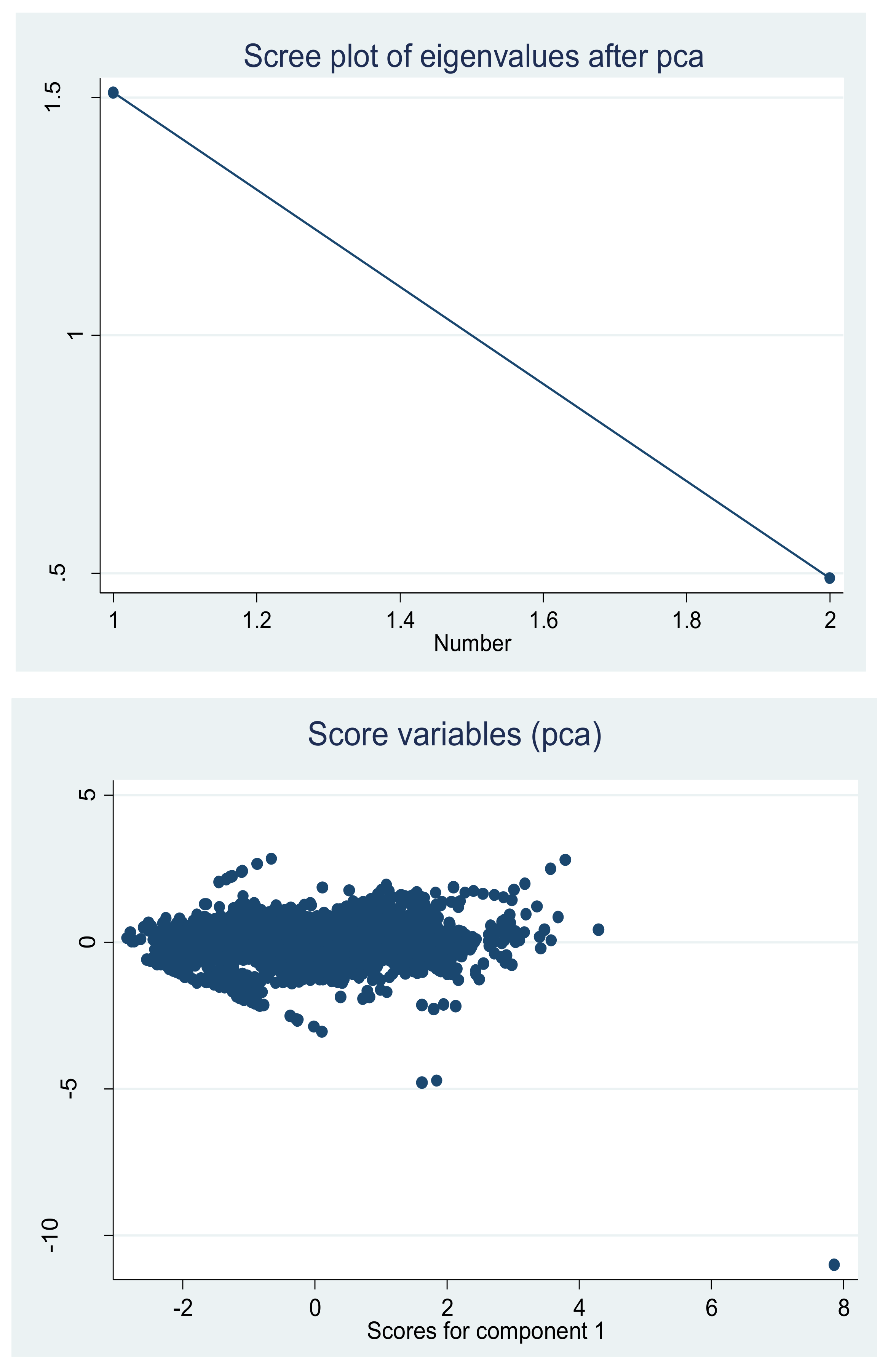
| Panel 1: Eigenvalues: (Sum = 2, Average = 1) | |||||
| Number | Value | Difference | Proportion | Cumulative Value | Cumulative Proportion |
| 1 | 1.510786 | 1.021572 | 0.7554 | 1.510786 | 0.7554 |
| 2 | 0.489214 | --- | 0.2446 | 2.000000 | 1.0000 |
| Panel 2: Eigenvectors (loadings): | |||||
| Variable | PC 1 | PC 2 | |||
| TR | 0.707107 | −0.707107 | |||
| GSP | 0.707107 | 0.707107 | |||
| Panel 3: Ordinary correlations: | |||||
| Variables | TR | GSP | |||
| TR | 1.000000 | 0.810786 | |||
| GSP | 0.810786 | 1.000000 | |||
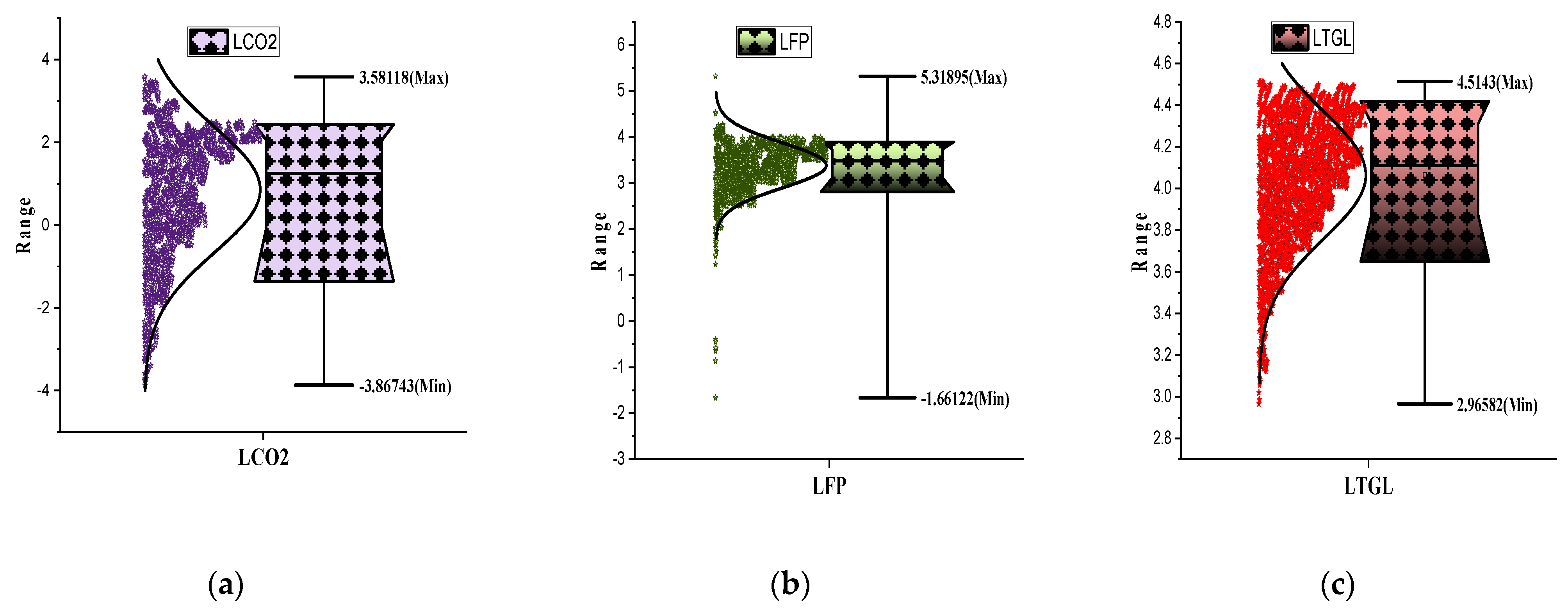
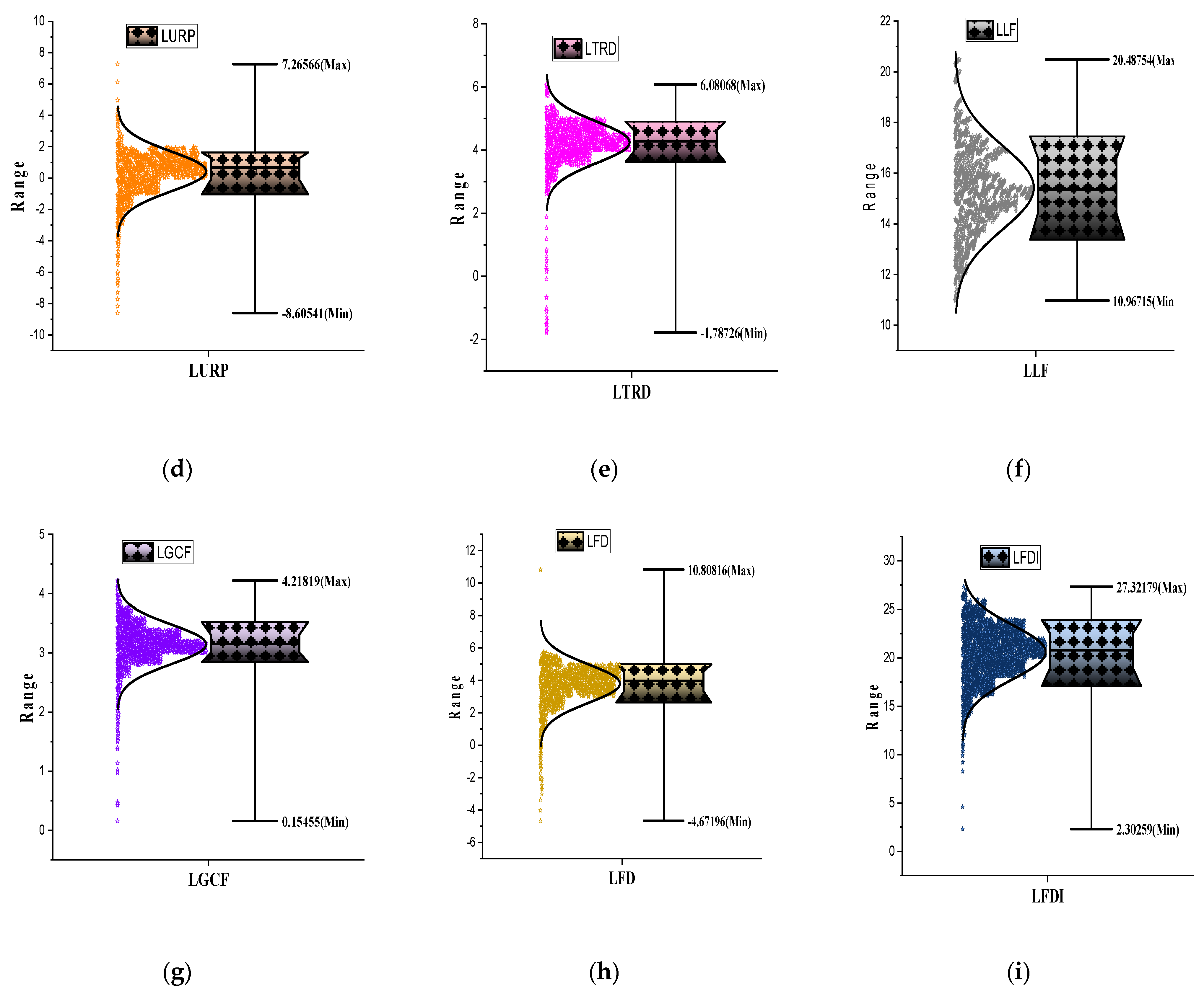
| Mean | Median | Maximum | Minimum | Std. Dev. | Skewness | Kurtosis | |
|---|---|---|---|---|---|---|---|
| LCO2 | 0.85362 | 1.24676 | 3.58117 | −3.86743 | 1.51485 | −0.73682 | 2.89665 |
| LFP | 2.61183 | 15.2137 | 3.88287 | −3.13511 | 0.664202 | −0.2371 | 2.02769 |
| LTGL | 4.06436 | 4.11082 | 4.51429 | 2.96582 | 0.30552 | −0.79715 | 3.27120 |
| LFDI | 20.5860 | 20.7805 | 27.3217 | 2.30258 | 2.78277 | −0.83094 | 5.77482 |
| LFD | 3.79566 | 3.95761 | 10.8081 | −4.67196 | 1.18458 | −1.74790 | 12.2953 |
| LTRD | 4.24519 | 4.28122 | 6.08068 | −1.78726 | 0.65404 | −2.96416 | 25.2427 |
| LURP | 0.42515 | 0.66434 | 7.26566 | −8.60548 | 1.26919 | −1.70453 | 10.1602 |
| LLF | 15.4299 | 15.3630 | 20.4875 | 10.9671 | 1.64369 | 0.21535 | 3.29817 |
| LGCF | 3.14435 | 3.14769 | 4.21819 | 0.15455 | 0.33534 | −1.78584 | 13.9852 |
| Variables | LCO2 | LFP | LTGL | LFDI | LFD | LTRD | LURP | LLF | LGCF |
|---|---|---|---|---|---|---|---|---|---|
| LCO2 | 1.0000 | ||||||||
| LFP | 0.2123 | 1.0000 | |||||||
| [11.566] | ----- | ||||||||
| (0.0000) | ----- | ||||||||
| LTGL | 0.6677 | 0.3926 | 1.0000 | ||||||
| [47.748] | [22.726] | ----- | |||||||
| (0.0000) | (0.0000) | ----- | |||||||
| LFDI | 0.5705 | 0.1622 | 0.7028 | 1.0000 | |||||
| [36.981] | [8.7506] | [53.410] | ----- | ||||||
| (0.0000) | (0.0000) | (0.0000) | ----- | ||||||
| LFD | 0.4008 | 0.2614 | 0.5404 | 0.3912 | 1.0000 | ||||
| [23.285] | [14.419] | [34.193] | [22.639] | ----- | |||||
| (0.0000) | (0.0000) | (0.0000) | (0.0000) | ----- | |||||
| LTRD | 0.1887 | 0.2425 | 0.2286 | −0.0059 | −0.0289 | 1.0000 | |||
| [10.231] | [13.366] | [12.499] | [−0.3143] | [−3.5434] | ----- | ||||
| (0.0000) | (0.0000) | (0.0000) | (0.7533) | (0.0000) | ----- | ||||
| LURP | −0.3674 | −0.2326 | −0.3889 | −0.2757 | −0.2188 | 0.0109 | 1.0000 | ||
| [−21.026] | [−12.733] | [−22.474] | [−15.267] | [−11.937] | [6.5845] | ----- | |||
| (0.0000) | (0.0000) | (0.0000) | (0.0000) | (0.0000) | (0.0000) | ----- | |||
| LLF | 0.0863 | −0.2311 | 0.1498 | 0.4869 | 0.1734 | −0.4591 | −0.1101 | 1.0000 | |
| [4.6121] | [−12.647] | [8.0676] | [29.677] | [9.3760] | [−27.512] | [−5.9004] | ----- | ||
| (0.0000) | (0.0000) | (0.0000) | (0.0000) | (0.0000) | (0.0000) | (0.0000) | ----- | ||
| LGCF | 0.1147 | 0.0291 | 0.0627 | 0.1251 | 0.0634 | 0.1266 | 0.0823 | 0.1794 | 1.0000 |
| [6.1493] | [1.5546] | [3.3475] | [6.7069] | [3.3825] | [6.7953] | [4.3975] | [4.0371] | ----- | |
| (0.0000) | (0.1201) | (0.0008) | (0.0000) | (0.0007) | (0.0000) | (0.0000) | (0.0000) | ----- |
| LLC | IPS | F-ADF | F-PP | |||||
| Variables | Stats. | Prob. | Stats. | Prob. | Stats. | Prob. | Stats. | Prob. |
| Level (Intercept and trend) | ||||||||
| LCO2 | −0.65089 | 0.3871 | −0.73300 | 0.2318 | 216.058 | 0.3725 | 141.052 | 0.7217 |
| LFP | −0.00518 | 0.6443 | −1.8809 | 0.1463 | 204.410 | 0.2188 | 102.936 | 0.8355 |
| LTGL | −1.98728 | 0.3263 | 1.29468 | 0.9023 | 192.859 | 0.2394 | 161.674 | 0.5214 |
| LFDI | −5.53230 *** | 0.0000 | 0.68817 | 0.9521 | 296.539 *** | 0.0001 | 506.880 *** | 0.0000 |
| LFD | 3.58481 | 0.9998 | −0.18932 | 0.7645 | 88.2352 | 0.7836 | 67.1559 | 0.9962 |
| LTRD | −3.56939 *** | 0.0000 | −3.85931 *** | 0.0000 | 343.679 *** | 0.0000 | 333.830 *** | 0.0000 |
| LURP | 2.2 × 10⁸ | 1.0000 | −1.28878 | 0.1195 | 367.402 *** | 0.0000 | 346.810 *** | 0.0000 |
| LLF | 1.80435 | 0.7862 | −0.15341 | 0.7139 | 153.830 | 0.2847 | 213.369 | 0.1533 |
| LGCF | −0.67731 | 0.2491 | −5.44384 *** | 0.0000 | 320.285 *** | 0.0000 | 450.360 *** | 0.0000 |
| First Difference (Intercept only) | ||||||||
| LCO2 | −17.7637 *** | 0.0000 | −25.1492 *** | 0.0000 | 1015.24 *** | 0.0000 | 1898.21 *** | 0.0000 |
| LFP | −23.6463 *** | 0.0000 | −28.7840 *** | 0.0000 | 1164.17 *** | 0.0000 | 1996.12 *** | 0.0000 |
| LTGL | −15.4499 *** | 0.0000 | −20.5946 *** | 0.0000 | 836.683 *** | 0.0000 | 1484.85 *** | 0.0000 |
| LFDI | −55.0309 *** | 0.0000 | −54.0598 *** | 0.0000 | 2138.94 *** | 0.0000 | 2363.50 *** | 0.0000 |
| LFD | −33.6540 *** | 0.0000 | −35.2921 *** | 0.0000 | 1452.82 *** | 0.0000 | 1549.49 *** | 0.0000 |
| LTRD | −29.4918 *** | 0.0000 | −29.0033 *** | 0.0000 | 1147.44 *** | 0.0000 | 1844.44 *** | 0.0000 |
| LURP | 3.4 × 10⁸ | 1.0000 | −19.6390 *** | 0.0000 | 800.199 *** | 0.0000 | 1113.88 *** | 0.0000 |
| LLF | −9.36101 *** | 0.0000 | −18.6859 *** | 0.0000 | 784.138 *** | 0.0000 | 1326.48 *** | 0.0000 |
| LGCF | −22.2136 *** | 0.0000 | −27.8403 *** | 0.0000 | 1131.70 *** | 0.0000 | 1883.46 *** | 0.0000 |
| Hypothesized | Fisher Stat. * | Fisher Stat. * | ||
| No. of CE(s) | (from Trace Test) | Prob. | (from Max Eigen Test) | Prob. |
| None | 1442.0 | 0.0000 | 1612.0 | 0.0000 |
| At most 1 | 3266.0 | 0.0000 | 1098.0 | 0.0000 |
| At most 2 | 1899.0 | 0.0000 | 1899.0 | 0.0000 |
| At most 3 | 5507.0 | 0.0000 | 2857.0 | 0.0000 |
| At most 4 | 3547.0 | 0.0000 | 1874.0 | 0.0000 |
| At most 5 | 2212.0 | 0.0000 | 1157.0 | 0.0000 |
| At most 6 | 1292.0 | 0.0000 | 735.90 | 0.0000 |
| At most 7 | 810.80 | 0.0000 | 612.50 | 0.0000 |
| At most 8 | 572.80 | 0.0000 | 572.80 | 0.0000 |
| Kao Test Statistics | t-Statistic | Prob. | ||
| ADF | −5.599249 | 0.0000 | ||
| Residual variance | 0.158971 | |||
| HAC variance | 0.131422 | |||
| Variable | Full Modified Least Squares (FMOLS) | Dynamic Least Squares (DOLS) | Autoregressive Distributed Lag (ARDL) | |||||||||
|---|---|---|---|---|---|---|---|---|---|---|---|---|
| Coeff. | Std. Err. | t-Stat. | Prob. | Coeff. | Std. Err. | t-Stat. | Prob. | Coeff. | Std. Err. | t-Stat. | Prob. | |
| LFP | 0.0017 * | 0.0008 | 2.0482 | 0.0406 | 0.0266 * | 0.0032 | 6.3052 | 0.0000 | 0.0193 * | 0.0018 | 10.5689 | 0.0000 |
| LTGL | 0.6036 * | 0.1046 | 5.7668 | 0.0000 | 0.5879 * | 0.0547 | 5.2186 | 0.0000 | 0.9787 * | 0.1123 | 8.7122 | 0.0000 |
| LFDI | 0.0204 * | 0.0032 | 6.2712 | 0.0000 | 0.1468 * | 0.0158 | 9.2905 | 0.0000 | 0.1014 * | 0.0096 | 10.5008 | 0.0000 |
| LFD | 0.0446 * | 0.0116 | 3.8362 | 0.0001 | 0.0791 ** | 0.0326 | 2.4218 | 0.0156 | 0.4592 * | 0.0309 | 14.8196 | 0.0000 |
| LTRD | −0.0629 * | 0.0235 | −2.6615 | 0.0078 | −0.2594 * | 0.0489 | −3.2139 | 0.0000 | −0.7733 * | 0.0414 | −18.6657 | 0.0000 |
| LURP | −0.2582 * | 0.0288 | −9.2180 | 0.0000 | −0.0869 * | 0.0287 | −3.0963 | 0.0020 | −0.1598 * | 0.0265 | −6.0067 | 0.0000 |
| LLF | −0.1358 * | 0.0293 | −4.6341 | 0.0000 | −0.0762 * | 0.0252 | −3.0454 | 0.0024 | −0.3527 * | 0.0123 | −28.3524 | 0.0000 |
| LGCF | 0.1661 * | 0.0182 | 9.1281 | 0.0000 | 0.4406 * | 0.0869 | 5.0684 | 0.0000 | 0.3652 * | 0.0724 | 5.0384 | 0.0000 |
| R-squared | 0.990386 | 0.927735 | Log likelihood | 3933.757 | ||||||||
| Adjusted R-squared | 0.898407 | 0.797611 | Akaike info criterion | −2.028752 | ||||||||
| Long-run variance | 0.009471 | 0.138633 | Schwarz criterion | 0.191666 | ||||||||
| Mean of dependent variable | 0.860372 | 0.844781 | Hannan–Quinn criterion | −1.227773 | ||||||||
| S.E. of regression | 1.324234 | 0.683089 | 0.114583 | |||||||||
| S.D. dependent variable | 1.507546 | 1.518392 | 0.133869 | |||||||||
| Sum squared residual | 4773.289 | 433.0149 | 23.33059 | |||||||||
| Variables | Coefficient | Std. Error | t-Statistics | Prob. * |
|---|---|---|---|---|
| COINTEQ01 | −0.431902 * | 0.014800 | −3.831271 | 0.0000 |
| D(LCO2(-1)) | −0.078158 * | 0.028397 | −2.752280 | 0.0060 |
| D(LFP) | 0.000129 | 0.001370 | 0.094115 | 0.9250 |
| D(LTGL) | 0.210432 | 0.191473 | 1.099019 | 0.2719 |
| D(LFDI) | 5.06 × 10⁻⁵ | 0.004113 | 0.012300 | 0.9902 |
| D(LFD) | 0.013383 | 0.020152 | 0.664082 | 0.5067 |
| D(LTRD) | −0.073211 *** | 0.042288 | −1.731229 | 0.0836 |
| D(LURP) | −0.148159 *** | 0.080229 | −1.846695 | 0.0650 |
| D(LLF) | 0.067043 | 0.248327 | 0.269980 | 0.7872 |
| D(LGCF) | 0.105450 * | 0.030123 | 3.500670 | 0.0005 |
| Single Threshold | Double Threshold | Triple Threshold | |
|---|---|---|---|
| F-statics | 115.21 | 23.63 | 17.63 |
| p-value | 0.0000 | 0.246 | 0.322 |
| Critical Values | |||
| 10% | 36.2299 | 32.1352 | 27.6806 |
| 5% | 42.5525 | 37.9405 | 33.6307 |
| 1% | 61.0479 | 51.8926 | 51.7746 |
| Bootstrap Repeat | 500 | 500 | 500 |
| Threshold Value | 95% Confidence Interval | |
|---|---|---|
| Lower Value | Upper Value | |
| −1.2289 | −1.2485 | −1.2213 |
Publisher’s Note: MDPI stays neutral with regard to jurisdictional claims in published maps and institutional affiliations. |
© 2021 by the authors. Licensee MDPI, Basel, Switzerland. This article is an open access article distributed under the terms and conditions of the Creative Commons Attribution (CC BY) license (https://creativecommons.org/licenses/by/4.0/).
Share and Cite
Kamal, M.; Usman, M.; Jahanger, A.; Balsalobre-Lorente, D. Revisiting the Role of Fiscal Policy, Financial Development, and Foreign Direct Investment in Reducing Environmental Pollution during Globalization Mode: Evidence from Linear and Nonlinear Panel Data Approaches. Energies 2021, 14, 6968. https://doi.org/10.3390/en14216968
Kamal M, Usman M, Jahanger A, Balsalobre-Lorente D. Revisiting the Role of Fiscal Policy, Financial Development, and Foreign Direct Investment in Reducing Environmental Pollution during Globalization Mode: Evidence from Linear and Nonlinear Panel Data Approaches. Energies. 2021; 14(21):6968. https://doi.org/10.3390/en14216968
Chicago/Turabian StyleKamal, Mustafa, Muhammad Usman, Atif Jahanger, and Daniel Balsalobre-Lorente. 2021. "Revisiting the Role of Fiscal Policy, Financial Development, and Foreign Direct Investment in Reducing Environmental Pollution during Globalization Mode: Evidence from Linear and Nonlinear Panel Data Approaches" Energies 14, no. 21: 6968. https://doi.org/10.3390/en14216968