Increasing Block Rate Electricity Pricing and Propensity to Purchase Electrical Appliances: Evidence from a Natural Experiment in Russia

Abstract

This paper provides empirical evidence on the relationship between the increasing-block-rate (IBR) pricing of electricity and the propensity of households to buy major electrical appliances. I use a variation from a natural experiment in Russia that introduced IBR pricing for residential electricity in a number of experimental regions in 2013. The study employs household-level panel data, which records, among others, whether the household has purchased any major electrical appliances during the last three months. Using a difference-in-differences specification, I show that the purchase of major electrical appliances in the regions with IBR pricing has increased by more than 20% (or more than two percentage points). The findings suggest that price-based energy policies may be an effective tool in shaping the behaviour of households.

1. Introduction

Characterising how consumers respond to energy prices has been an important avenue of research for the last fifty years. In particular, the extent to which consumers invest in energy-efficient appliances following the changes in energy pricing policies has had important implications for carbon mitigating policies.

The so-called energy efficiency paradox states that people underinvest in energy-efficient technologies, which can provide a low-cost solution to reducing CO₂ emissions and even provide positive returns in the form of reduced energy bills [1,2].

The studies analysing the decision to purchase energy-efficient appliances gained heightened interest after concerns regarding environmental deterioration started to grow in the second half of the 20th century. Investing in energy-efficient home appliances is one of the main channels for investment in energy efficiency. One of the first to study and model the consumer decision to purchase and use energy durables was Hausman [3]. In his seminal paper, he concluded that households value but substantially discount future energy savings when making purchase decisions. Gately [4] provided a similar analysis on a sample of refrigerators and arrived at a similar conclusion.

Dubin and McFadden [5] analysed behaviour when purchasing heating systems using a sample of 3249 households and confirmed the previous studies’ findings. They also found that consumers value but substantially discount and thus undervalue the future energy costs provided by energy-efficient appliances.

Contrary to the previous findings, Rapson [6] documented that consumers were more forward-looking than previously thought and took into account the future savings realised by the energy-efficient appliances. Moreover, the author concluded that consumer demand for electrical appliances (air conditioners in particular) was more elastic for energy efficiency than the up-front price of the durable.

Houde and Aldy [7] investigated the impact of the 2009 energy efficiency rebates program in the US. They found that rebates do not force consumers to increase investment in energy-efficient appliances. The authors explained this result by a high proportion of “free riders”, consumers who would have upgraded to energy-efficient appliances even without the rebates program, and an “income effect”, meaning that the rebates received by the consumers induced them to buy bigger and more energy-intensive units of appliances, a phenomenon closely related to the rebound effect.

Taking into consideration the supply side of the production decision Cohen and colleagues [8] showed that the existing energy efficiency gap in the home appliances market was not only due to the consumer myopia but also to the producers pricing appliances that are less energy-efficient more favourably. Moreover, the authors documented that manufacturers changed their product portfolio in response to the rising electricity prices. The authors concluded that shifting attention towards the producers would help achieve energy efficiency gains in the durables market.

Some authors also investigated whether the price of electricity and its structure affected a household’s decision to invest in energy-efficient technology. In particular, Jacobsen [9] investigated whether electricity prices affected the investment in energy-efficient appliances using state-year panel data on electricity prices and the proportion of sales of new appliances that involve high efficiency “Energy Star” models in the US. The collective set of results indicated that changes in electricity prices were not positively associated with changes in the market share of Energy Star appliances. Similar to Jacobsen [9], Borenstein [10] found that the “time of use” (TOU) pricing schedule did not have any substantial effect on the household’s decision to install solar PVs.

In a closely related study, Liang et al. [11] investigated the relationship between the electricity tariff structure and investment in energy-efficient appliances and solar panels using household-level data in Phoenix, Arizona. In particular, the authors found that the consumers who adopted the time-of-use (TOU) electricity pricing were 27% more likely to adopt solar panel installations but not more likely to invest in energy-efficient air conditioning. The authors, however, also concluded that their results should be interpreted as correlations and did not claim any causal relationship due to the lack of plausibly exogenous variation.

In my study, I combined the Russian Longitudinal Monitoring Survey (conducted by a Higher School of Economics) (RLMS-HSE), a household-level panel data, with a variation in electricity tariff that has resulted from a natural experiment in Russia to estimate the relationship between increasing-block-rate (IBR) pricing and the propensity of consumers to purchase electrical appliances. I found that households that faced IBR pricing were more than 20% (or more than two percentage points) more likely to purchase major electrical appliances.

Although I have not observed any energy efficiency indicators for the appliances, taking into account the robust trend of newer appliances becoming more energy-efficient [12,13], it is possible to propose that consumers purchasing new electrical appliances are also purchasing more energy-efficient appliances. Using this proposition, the results of this paper can potentially suggest that price-based energy policies are an effective tool not only in shaping the household’s behaviour but also in shaping the behaviour towards higher energy efficiency, which is considered one of the lowest-cost opportunities for reducing carbon emissions.

To the best of my knowledge, this is the first study that has combined household-level panel data with a variation resulting from a natural experiment to estimate the relationship between IBR pricing and the propensity of households to purchase electrical appliances. Therefore, this paper can potentially close an important gap in the literature.

The rest of the paper is structured as follows. In the following section, I presented some background information on the electricity market in Russia and described the natural experiment. Section 3 presents the data and the description of the selected sample. Section 4 outlines the methodology of the study, while Section 5 summarises the results. Section 6 is the conclusion.

2. The Electricity Market and the Natural Experiment

Until 2003, the entire power market was regulated by RAO UES, a fully integrated state monopoly. The RAO UES, however, had been unbundled into 20 independent power companies by 2008, after the power sector began to liberalise. However, there has been a resurgence in power asset acquisition in recent years. Russian Grids (PJSC), a state-controlled public joint-stock company, consolidated the vast transmission and distribution assets. Russian Grids owns and operates most power grids currently, with transmission and distribution of power to over 70% of the Russian population and industrial facilities accounting for over 60% of Russian GDP [14,15] (With a gross capacity of 243GW, Russia has the world’s fourth-largest electric power grid. Thermal power plants, which operate almost entirely on natural gas and coal, produce the majority of the electricity (about 67%). Hydroelectric power plants (20%) and nuclear power plants (12%) provide the remaining 30% [14,15]).

Electricity pricing has been increasingly liberalised, and about 80% of electric power is now traded on the open market at non-regulated market rates. However, in the near future, the public is likely to continue to purchase electric power at state-regulated rates, including residential tariffs set by the Federal Antimonopoly Service [14].

In Russia, residential electricity pricing is still largely based on a flat tariff system, though with a significant regional variance in price per kilowatt. In a recent effort to implement a cross-subsidising system, in which households with higher electricity usage cross-subsidise households with lower electricity consumption, Russia began implementing a social norm for electricity use in several pilot regions in September of 2013, with plans to expand the social norm to all Russian regions by July 2014 [16]. Households that consume less than the prescribed social norm pay a subsidised lower price, whereas households that consume more than the prescribed social norm pay a higher market price.

The social norm for electricity consumption is based on household per capita electricity consumption and is different in each of Russia’s seven experimental regions. The social norm varies from 50 kWh per capita in Vladimir Oblast to 190 kWh per capita in Orlov Oblast [17].

The estimation of the social norm has also been complicated (in some of the experimental regions) by such factors as the location of the household (whether it is in a rural or urban area), whether it has an installed electric stove, or the presence of individuals receiving benefits within the household (see

Table 1. Prescribed Social Norm for Electricity Consumption.

Region	Rostov			Krasnoyarsk			Nizhny Novgorod
HH Type	n = 1	n = 2	n = 3+	n = 1	n = 2	n = 3+	n = 1	n = 2	n = 3+
urban	96	156	156 + 40 × (n − 2)	110	150	75 × n	85	100	100 + 50 × (n − 2)
rural	186	246	246 + 40 × (n − 2)
urban + electric stove	186	242	156 + 40 × (n − 2) + 43 × n	220	300	150 × n	85	100	100 + 50 × (n − 2)
rural + electric stove	276	332	246 + 40 × (n − 2) + 43 × n
receiving social benefits	×1.5	×1.5	×1.5	×1.0	×1.0	×1.0	85	×1.5	×1.5

Source: Regional electricity suppliers; Note: “n” denotes the household size.

), among others.

Despite the complexities, the introduction of the social norm serves the same purpose as the increasing block rate tariff (IBR) in other countries. Consumption below a certain threshold is charged at a lower rate, whereas consumption above that threshold is charged at a higher rate. In these experimental regions thus, we deal with a two-block tariff regime.

Although the social norm was intended to be implemented across all Russian regions, it was postponed indefinitely due to a variety of factors [17,18]. Furthermore, two of the proposed nine pilot regions (Primorsky Krai and Lipetsk Oblast) opted out of the experiment before the social norms were piloted in seven regions in September 2013. The argument against implementation was that the federal government’s methodology for calculating the social norm was somewhat ambiguous, as shown by significant variations in social norm across some of the experimental areas, even though some had virtually the same weather and socioeconomic conditions [17]. As a result, one might argue that the social norms were prescribed practically exogenously, favouring our estimation procedures.

Even though the tariff based on a social norm was introduced overall in seven Russian regions, RLMS-HSE has not been conducted in all of them. Out of the seven regions that took part in the experiment (in particular, these regions are Zabaykalsky Krai, Krasnoyarsk Krai, Vladimir Oblast, Nizhny Novgorod Oblast, Oryol Oblast, Rostov Oblast, and Samara Oblast), RLMS-HSE was conducted in Rostov Oblast, Krasnoyarsk Krai, and Nizhny Novgorod Oblast. 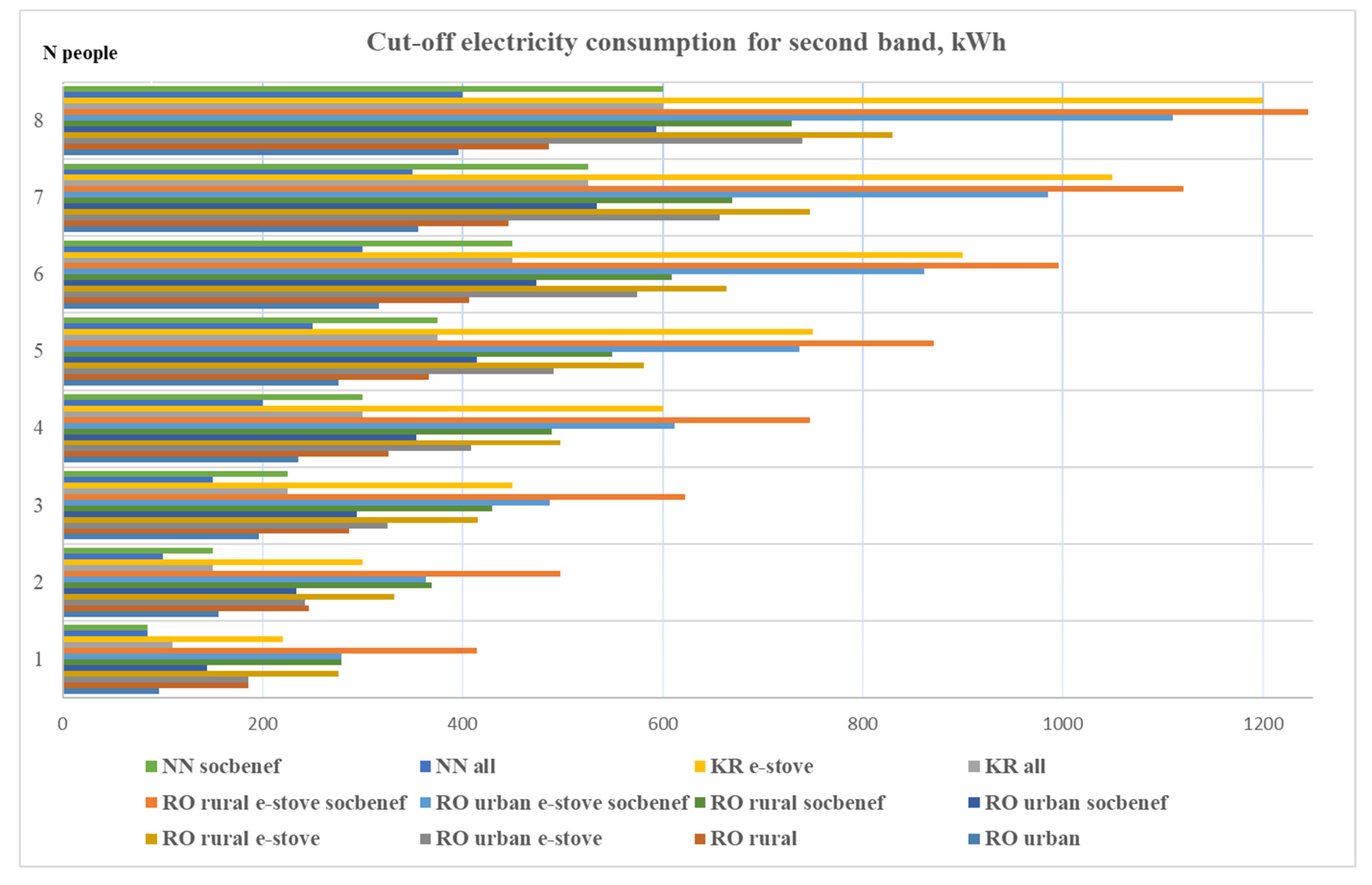Table 1 and Figure 1 below summarise the main information (the regional social norms for residential electricity consumption were obtained from the regional energy suppliers) regarding the social norms (in KwH) in these three regions of Russia [19,20,21].

Note: Since in Nizhny Novgorod (NN), the second band cut-off differs only for households with social benefits, the graph depicts the second band cut-off for all households and those on social benefits. The same reasoning applies to Krasnoyarsk (KR), where the graph depicts cut-offs for households with electric stoves and all others. On the other hand, the calculation of the cut-off in Rostov (RO) is more complex and depends on such factors as location (rural or urban), electric stove, social benefits, and all possible combinations of these three factors.

3. Data

3.1. RLMS-HSE

The paper employs the Russian Longitudinal Monitoring Survey (RLMS) conducted by the National Research University Higher School of Economics (HSE) and the Carolina Population Center at the University of Carolina [22]. RLMS-HSE is panel data and includes a wide set of questions on individual and family background characteristics. The majority of the interviews were conducted once a year during October and November in 38 major regions of Russia starting from 1994. It has administered to about 6000 households each year.

Although appliance data are rather detailed, the structure of the questionnaire on household appliances was adjusted in 2006 and 2009. For instance, starting from 2006, questionnaires collected information only on a new type of refrigerator (no-frost) and a new type of washing machine (automatic washing machine), as opposed to previous years when information on any type of refrigerator or washing machine was recorded. Since 2009, the questionnaire has added additional questions on the availability of air-conditioners (AC) and dishwashers, which were unavailable in previous years. Therefore, in this paper, I used the data for the period of 2010 to 2019.

RLMS-HSE contains detailed information on the socioeconomic characteristics of the household and information on any form of subsidies and discounts on utilities received by the household.

In the context of Russia, subsidies are short-term benefits given mostly on the basis of household income, in particular, the share of the total utility payments compared to the total income of the household. Any citizen with a permanent registration can apply for the subsidy. This subsidy is given for six months, and every six months, it needs to be renewed. The subsidy is given in the form of a cash-back payment. The household pays the monthly utility bill as usual, and then the payment for the bill is partially returned to the household by the government in the form of a cash-back payment [23,24].

Discounts, on the other hand, are given for the long term, and only certain segments of the population are eligible for them. These segments include but are not limited to war veterans, people with disabilities, and large families with children. The discounts are usually given in the form of reduced payment for the utility (a discount) and granted for a lifetime (in the case of veterans and the disabled), or until the youngest child from a large family turns sixteen or eighteen, depending on the region [23,24].

We can also identify whether the dwelling is in a multifamily or single-family building and whether it is connected to a central delivery of electricity, gas, water, hot water, and heating. The size of the dwelling (in square metres) is divided into a total area and the area of the living rooms. Moreover, the respondents are asked to indicate whether they own the apartment they live in.

The questionnaire also asks participants to indicate all major electrical appliances available within the household and whether the household has purchased any major electrical appliances in the last three months. Unfortunately, the questionnaire does not ask participants to specify which particular appliance (if any) the household has purchased and the energy efficiency rating of any of the given appliances.

Furthermore, the sampling approach of RLMS-HSE, combined with frequent (annual) replenishment, ensures that the sample is cross-sectionally representative for each round. The average attrition rate is about 10%, and the overall attrition after ten years is about 50% [25].

3.2. Descriptive Statistics

For the selected years (2010–2019), we obtained a total of 53,040 observations (This excludes all households which do not own the dwelling they reside in (e.g., renters). As in other post-Soviet countries, homeownership in Russia is high. In our particular sample, it is more than 91%). About 9% (4768) are households in treatment regions. Below is presented the summary statistics for treatment and control households.

We can observe (see

Table 2. Characteristics of the Dwelling.

Variables	Control Regions: Percentage of the Sample or Mean (Standard Deviation in Parentheses)	Treatment Regions: Percentage of the Sample or Mean (Standard Deviation in Parentheses)	Difference in Means: Standard Error in Parentheses
Type of dwelling:
Single-family home	27.1%	21.8%	5.3% ***
Apartment in multi-family building	72.6%	77.9%	−5.3% ***
Size of the dwelling in square metres	56.33 (23.65)	54.63 (20.30)	1.699 *** (0.325)
Urban	67.2%	94.0%	−26.8% ***
Has an Electric stove	19.7%	37.4%	−17.7%
Electricity consumption # (September)	179.11 (109.80)	185.88 (98.39)	−6.77 *** (1.946)
Has central delivery of:
Gas	70.1%	52.2%	17.8% ***
Heating	70.3%	77.4%	−7.2% ***
Hot water	65.0%	75.0%	−10% ***
Cold Water	88.1%	91.9%	−3.8% ***

* p < 0.1, ** p < 0.05, *** p < 0.01; Source: Author’s own calculations; ^# The data for electricity consumption is available only up to 2016.

and

Table 3. Household’s Socioeconomics.

Variables	Control Regions: Percentage of the Sample or Mean (Standard Deviation in Parentheses)	Treatment Regions: Percentage of the Sample or Mean (Standard Deviation in Parentheses)	Difference in Means: Standard Error in Parentheses
Household size	2.743 (1.49)	2.825 (1.42)	−0.083 *** (0.021)
Household monthly income (RU)	65,190.51 (57,276)	65,484.42 (45,529)	293.91 (775.07)
Receiving discounts for utilities	28.3%	27.7.0%	0.6%
Receiving subsidies for utilities	17.8%	18.6%	0.7%
Have Debt for Utilities	7.6%	7.1%	0.5%
Education:
Secondary	33.4%	29%	4.3% ***
Professional-technical	23.6%	24.8%	1.2% *
Higher education (MSc, BSc, DiS)	24.5%	26.7%	−2.2% ***
Other	18.2%	19%	0.8%

* p < 0.1, ** p < 0.05, *** p < 0.01; Source: Author’s own calculations.

) that there are some differences across the two samples in terms of observed characteristics. The most distinct difference that we observe across the two samples is that the experimental dwellings are located in more urbanised areas, whereas the households in the control group are less urbanised. The urbanisation level of the treatment group is 94%, whereas, in the control group, it is slightly above 67%.

This difference in urbanisation, in turn, is reflected in several other variables of interest. Central delivery of gas is about eighteen percentage points higher in the control group (52% vs. 70%). This, in turn, is reflected in a higher percentage of installed electric stoves in treatment regions, 37.4%, as opposed to about 20%.

Other observed characteristics are fairly similar. The descriptive statistics show that the majority of the families reside in multi-apartment buildings. The average size of the dwelling is about 55 m², while the average number of people residing in the dwellings is less than three individuals. Almost 30% of the households are receiving some benefits for utilities. The average household income is about 65,000 rubles (adjusted for 2019).

Below (see

Table 4. Major Appliances.

	Control Regions	Treatment Regions	Difference in Means:
Appliance	Percentage of the Sample
Air Conditioner	9.4%	10.1%	−0.7% *
Dishwasher (automatic)	3.8%	2.6%	1.2% ***
Refrigerator (no frost)	58.2%	61.5%	−3.4% ***
Washing machine (automatic)	79.3%	85.3%	6% ***
Freezer	13.7%	22.2%	−8.5% ***
Microwave	66.8%	67.3%	0.5%

* p < 0.1, ** p < 0.05, *** p < 0.01; Source: Author’s own calculations.

), the households’ appliances decomposition for 2010–2019 is reported. The only major difference that we observed is that the share of households owning a separate freezer is eight-point-five-percentage points higher than the control regions.

As can be seen, there are some observable differences across the groups. This can potentially bias our DiD estimations framework. I addressed this issue by applying a coarsened exact matching procedure prior to the estimations (see the Methodology section for details).

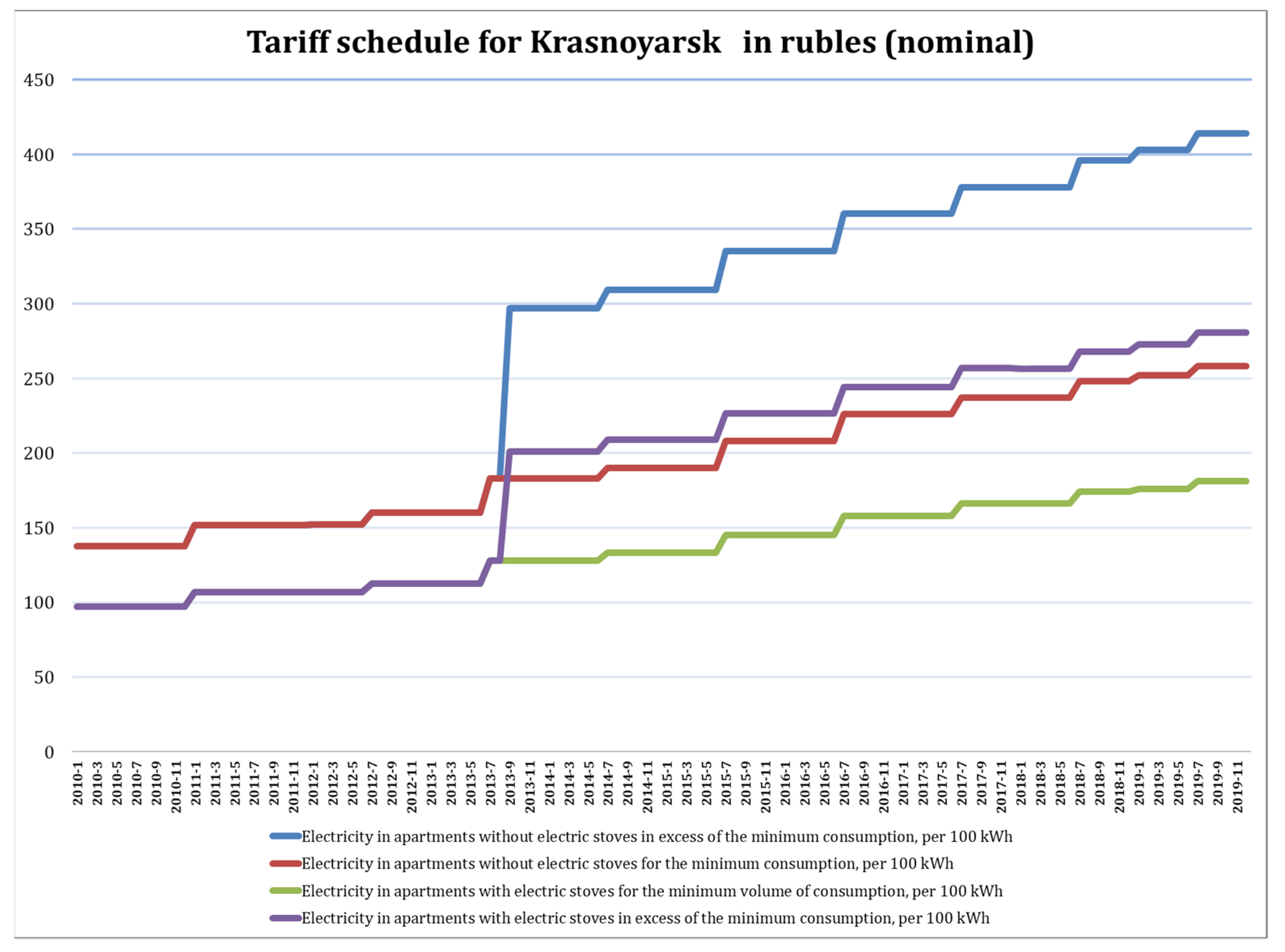
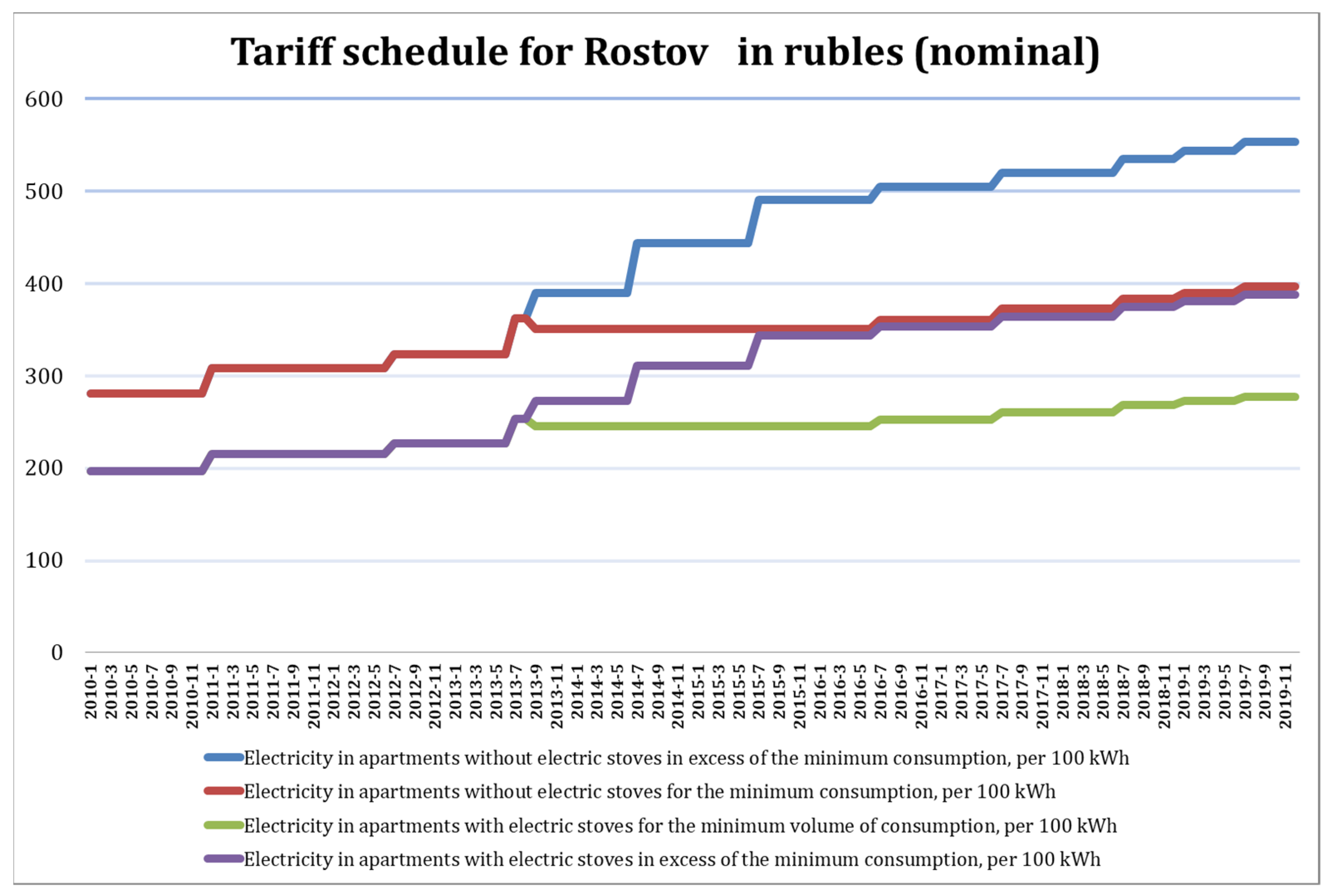
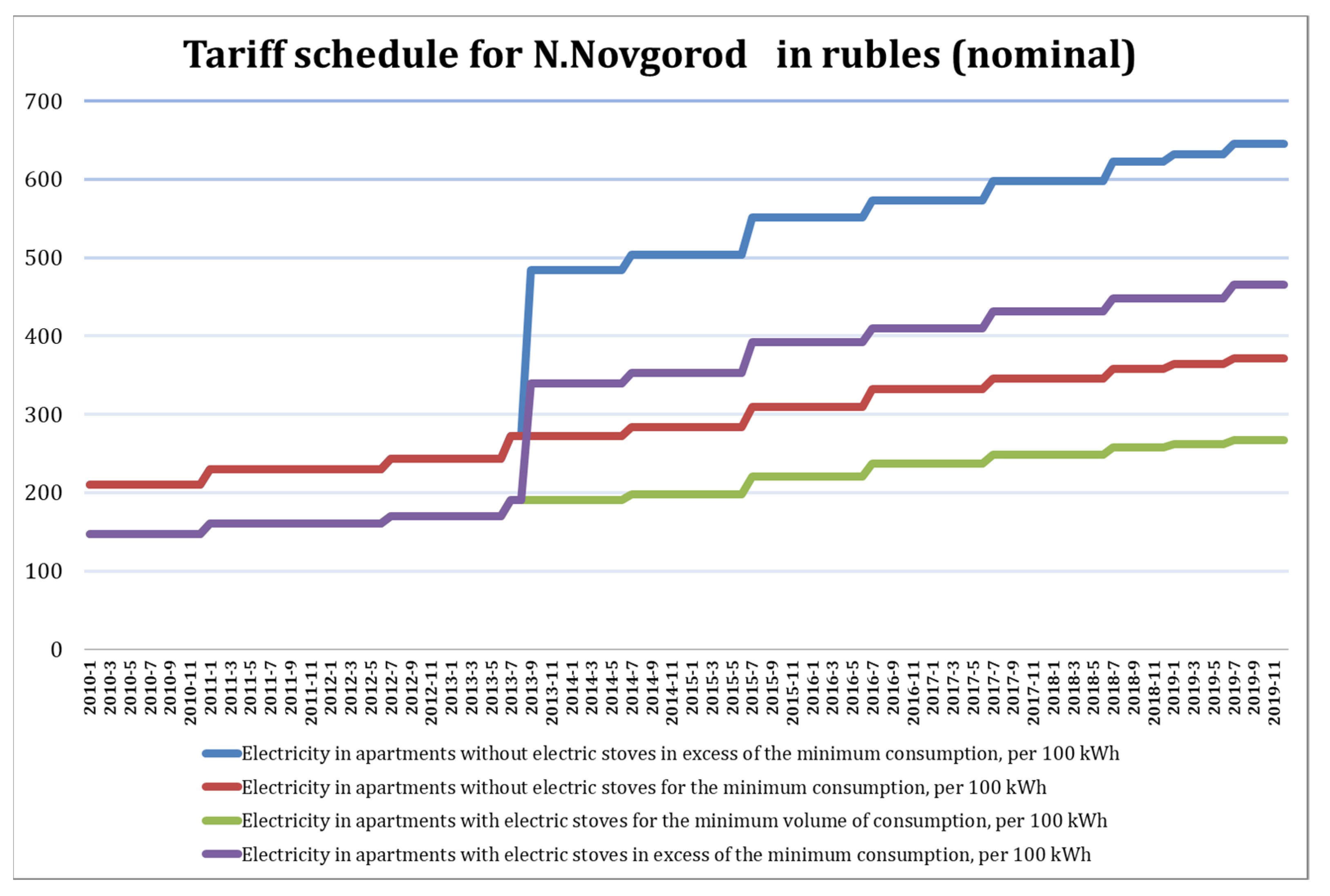
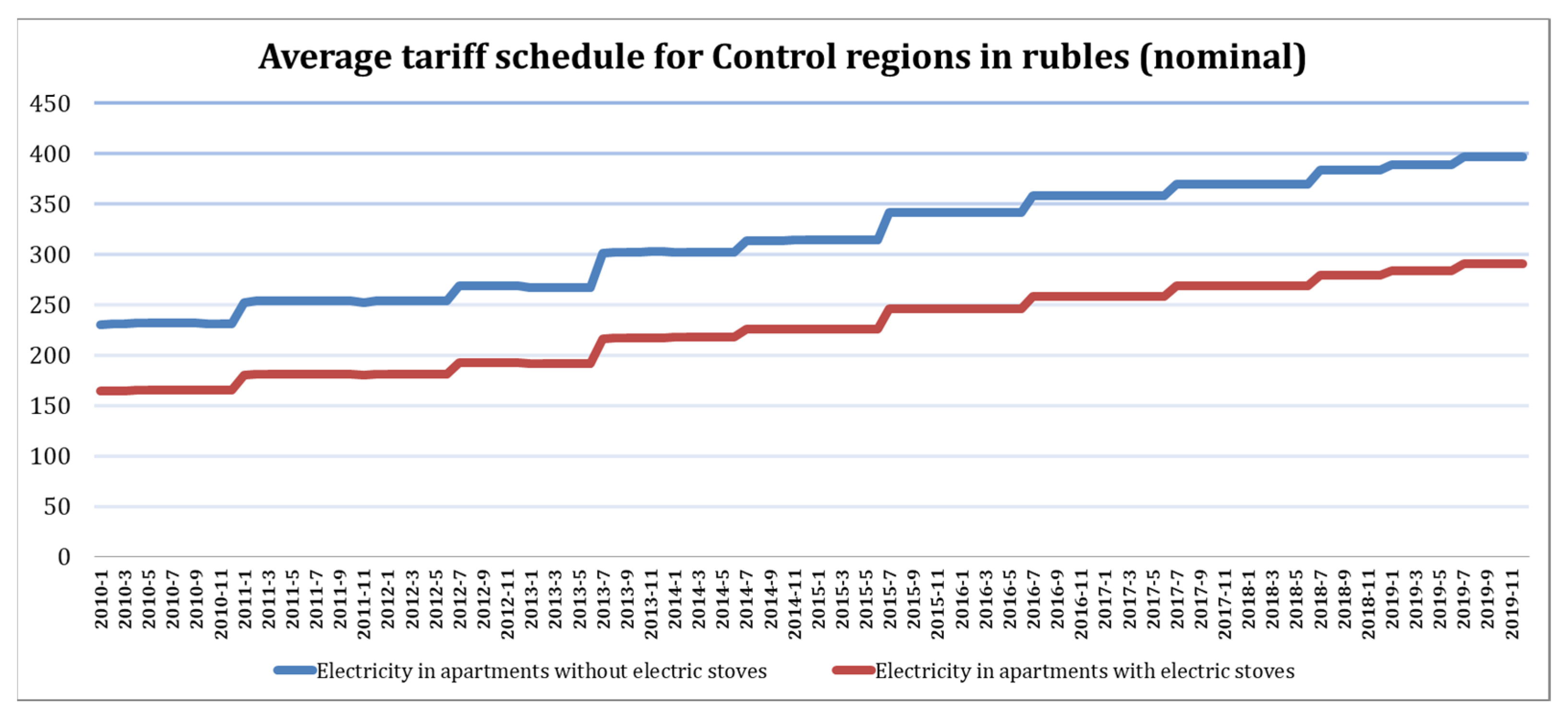
In addition to the variation in social norms, we also observed a considerable variation in electricity tariffs across both experimental and control regions. I illustrated the monthly tariff schedule for each of the experimental regions and the average tariff schedule for control regions for the period of 2010–2019 in the figures presented in Appendix A. The monthly electricity tariff data were obtained from the Russian statistical agency, “Goskomstat” [26].

The tariff schedule in Russia usually changes once a year and simultaneously in all regions. It varies substantially across regions, depending mostly on the average income of the population and weather conditions. It also usually varies between residential customers who, for various reasons, do not have access to the central gas supply and those who have a central delivery of gas. This is because households without a gas supply are forced to use electric stoves for cooking, which in turn increases their electricity consumption substantially. Thus, we dealt with two different tariffs between 2010 and 2013 (a flat tariff for households with an electric stove and a flat tariff for those without), and four tariffs after the introduction of a social norm in three experimental regions (1st and 2nd tiers for households with electric stove, and without). Undoubtedly, there may be households that do have access to a central gas supply but still prefer to install electric stoves at home. However, out of about 21% of households with installed electric stoves, less than 1% reported both access to central gas delivery and had installed electric stoves at home.

The average tariff for the first tier across all regions under the study increased from about 235 rubles per 100 kWh in 2010 to 409 rubles in 2019. The first-tier tariff in experimental and control regions followed roughly the same pattern, increasing from 191 rubles to 321 rubles and from 240 rubles to 418 rubles, respectively, during the same period.

Tariffs for the second tier could be observed in only three experimental regions under the study starting from September of 2013. The average tariff for the second-tier consumption (consumption above prescribed social norm) in three experimental regions grew from 366 rubles per 100 kWh in 2013 to 512 rubles per 100 kWh in 2019.

Tariff schedules for the households with electric stoves both in control and experimental regions followed an identical pattern, with a factor of roughly 0.7.

4. Methodology

In this study, I employed a “difference in difference” estimation to evaluate the effect of increasing block pricing on the investment in electrical appliances. The empirical model is estimated by Equation (1) via fixed effects regression (the Hausman specification test rejected the random effects model at all conventional levels in favour of the fixed effects model):

$$I{A}_{it}=a_i+{\tau }_t+X_{it}{b}_1+ln{P}_{it}{b}_2+ln{S}_{it}{b}_3+\left(treatment\ast post\right)b_4+{\epsilon }_{it}$$

(1)

On the right-hand side, we have time-varying control variables, household, and year fixed effects. As we are estimating the investment in electrical appliances in the context of natural experiment, we also should include variables indicating whether the region is a part of the experimental IBR tariff regime (treatment), whether the region was observed before or after the introduction of the IBR (post), and the interaction of these two variables (treatment ∗ post). In the difference in difference (DID) context, the coefficient of the interaction term is the DID estimator that the researcher tries to estimate.

However, because my model includes individual fixed effects, and the treatment is time-invariant, I did not include the main effect of treatment. Moreover, because I included time-fixed effects, including a dummy indicator for the post-intervention period is redundant.

The term $lnP$ stands for the log of the average residential price (in 2019 Russian rubles) for electricity. The price has both time and household subscripts to account for the price variability across years and regions. Because the household’s electricity consumption in RLMS-HSE is observed only for one month in a year (September), I used the average prices of electricity rather than the marginal prices. The use of average prices is justified not only by data limitations but also by recent empirical evidence that consumers react to average prices rather than marginal ones [27,28].

$lnS$ is a vector of the (log) amount (in 2019 Russian rubles) of any benefits (subsidies and discounts) for the utilities received by the household. $X$ is a vector of control variables like the household’s income (in 2019 Russian rubles) and the number of individuals residing in the household. The terms $a_i$ and ${\tau }_t$ stand for household fixed effects and year fixed effects, respectively.

Our dependent variable, $I{A}_{it}$, is a binary indicator for the purchase of any major electrical appliance within three months by a household $i$ in year $t$.

To be more precise, the questionnaire asks respondents if the household has purchased any energy-intensive electrical appliances during the last three months. The exact formulation of the question is as follows:

“Has your family bought any household appliances in the last three months, such as a refrigerator, washing machine, vacuum cleaner, sewing machine, iron, food processor, and the like?”

(Hse.ru. “Wave 19 Household Data File”, 2010, p. 205 [29]).

In order to avoid ambiguity, the questionnaire also asks if the household has recently purchased any non-major appliances. The exact formulation of the question is as follows:

“Has your family bought any recreational appliances in the last three months such as a TV, tape recorder, video recorder, musical instruments, computer, camera and the like?”

(Hse.ru. “Wave 19 Household Data File”, 2010, p. 205 [29]).

Thus, we can differentiate between the purchase of energy-intensive major appliances and other recreational non-major appliances.

The binary nature of our dependent variable implies that running the Ordinary Least Squares (OLS) analysis on this difference-in-differences specification will result in a linear probability model (LPM) estimation. An LPM model specification has several advantages compared to some other index model alternatives such as Logit or Probit. It is more convenient, computationally tractable, and may even have less bias than other nonlinear model alternatives, especially in the context of panel data [30].

Although LPM in the context of panel data is often considered to be a better alternative to its nonlinear counterparts, any regression outcomes estimated by LPM can suffer from two potential problems attributable specifically to LPM.

The first problem is that OLS suffers from heteroskedasticity when estimated on a binary response variable. This problem, however, is easily solved by employing heteroskedasticity robust standard error estimates.

The second problem is more complex and related to the fact that LPM estimates are not constrained to the unit interval. Thus, one can obtain estimates of probability that are above one or below zero. However, as argued by Wooldridge [31], when the main purpose is to estimate the partial effect on the response probability, averaged across the distribution of the independent variable, the fact that some predicted values lie outside the unit interval may not be that important (p. 455). Moreover, as shown by Horrace and Oaxaca [32], if no (or very few) predicted probabilities lie outside the unit interval, then the LPM is expected to be unbiased and consistent (in our case, only less than 0.5% of all predicted probabilities lie outside the unity interval in all model specifications that were estimated).

I also did not observe the energy efficiency of the electrical appliances purchased by the household. However, there is evidence that over a period of twenty to thirty years, the average improvements in energy efficiency can be up to 200% for a refrigerator, 50% for a room air conditioner, 65% for a standard freezer, and up to 100% for washing machines, and dishwashers [12,13]. Therefore, in this study, I assumed that for selected home electrical appliances, newly purchased appliances result in improvements in energy efficiency.

When the researcher tries to estimate the price elasticity of electricity demand in the case of nonlinear tariffs, such as in the presence of block pricing schemes, both marginal and average prices are endogenous [33]. A well-accepted method for dealing with endogenous marginal (average) prices under nonlinear price schedules when estimating the price elasticity of electricity demand (when the dependent variable is usually a log of electricity consumption) is to instrument for (log) the price with the (log) full block-tariff schedule [34,35].

In this case, however, I did not estimate the price elasticity of electricity demand, and the dependent variable used in this study is a binary indicator for the purchase of electric appliances. This, in turn, should not result in a correlation between the electricity price and the error term in Equation (1).

However, to minimise any endogeneity concerns, I also run the model above with instrumenting for the log of the average price of electricity by the full block-tariff schedule.

Additionally, I combined the model above with a coarsened exact matching (cem) procedure to address the differences in the major household characteristics across the treatment and control groups. Applying matching to any particular estimator usually serves as a tool to reduce the imbalance between treatment and control groups so that the empirical distribution of the covariates is more similar across the groups. The cem estimator has several advantages over other matching techniques. It requires fewer assumptions and possesses more attractive statistical properties [36].

I matched treatment and control groups based on the various household characteristics. More specifically, I matched based on the square footage of the dwelling, size of the household, its type (single-family or multi-apartment), location (urban, rural), household income, and whether the household is connected to the central delivery of hot water, and central heating.

5. Results

5.1. Preliminary Data Checks

The key assumptions of the DID estimation technique are the “parallel trends” and the “common shocks” assumptions [37]. In other words, if the treatment had been absent itself, the treatment and control regions would have followed the same trends. That is, any omitted variables affect the treatment and control in the same way. Usually, these assumptions are tested by examining the outcome variable over time for treatment and control groups.

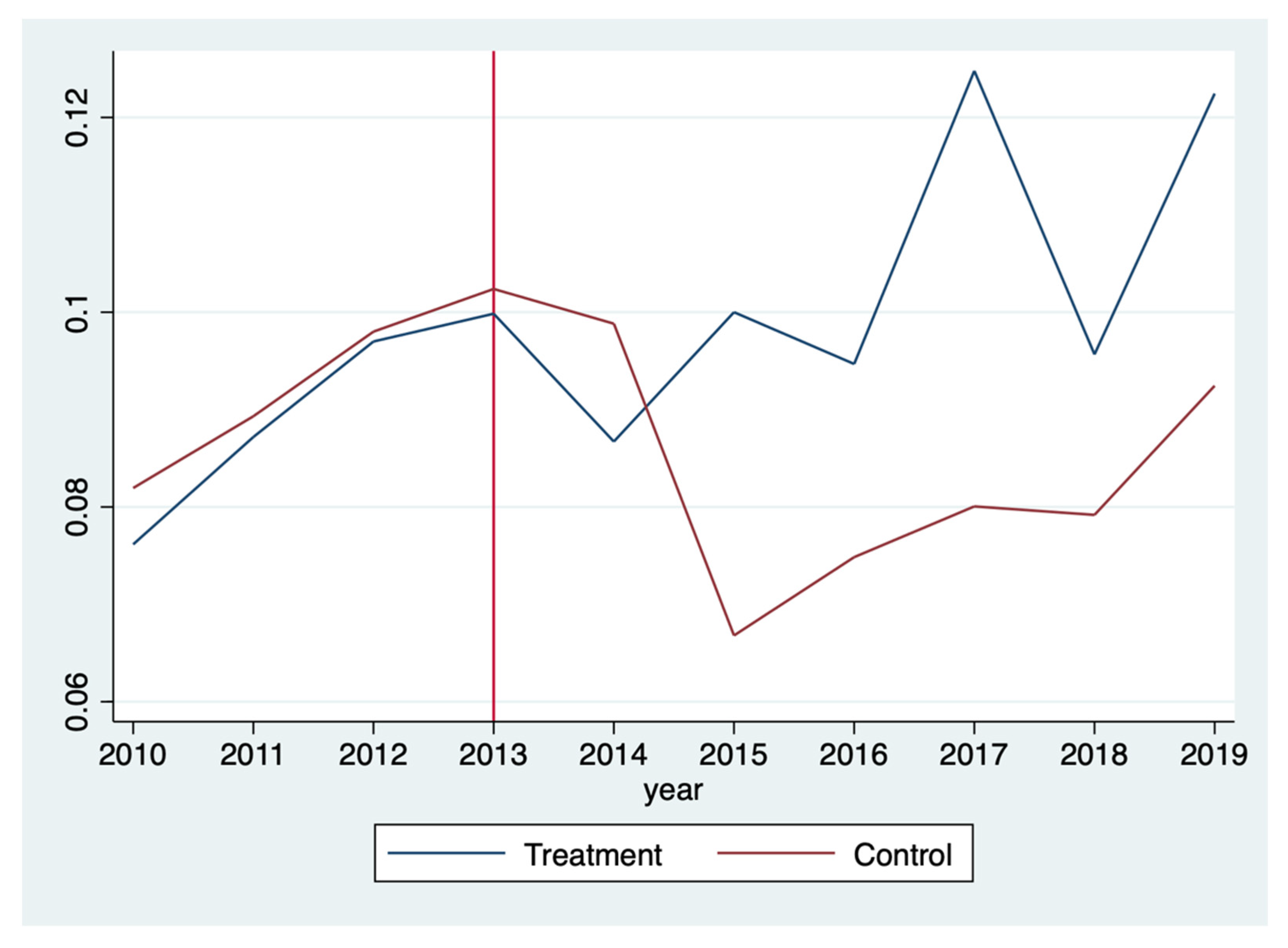
Figure 2 below plots the propensity to purchase major electrical appliances for the households in the control and treatment regions for the period of 2010–2019.

We can see that the purchase of major electrical appliances was gradually increasing prior to 2014 in both the treatment and control regions and went downward in 2014.

The drop of 2014 may potentially indicate that the households were forming “expectations” and hedging towards uncertainty due to the conflict of Russia with Ukraine and postponed the purchase of electric durables. The more pronounced decline of 2015 observed in the control regions followed after the imposition of economic sanctions by the international community in December of 2014 [38] (The imposition of the sanctions also resulted in a severe devaluation of the Russian ruble. By January of 2015, the Russian ruble had devalued by more than 100% against the USD and 60% against the EUR compared to January of 2014 [38]. Since most of the electronics are imported in Russia, this sharp devaluation increased the cost of all imported electric durables considerably).

Taking into consideration that the decision to purchase home electrical appliances is considered a major investment by many households in Russia, we anticipated that consumers would react to the treatment with some time lag.

Indeed, we observed that trends in the treatment and control regions started to diverge in 2015 (two years after the introduction of IBR tariffs) when the propensity to purchase electrical appliances grew in treatment regions by one point five percentage points. In contrast, in the control regions, as mentioned above, it actually fell by more than three percentage points.

Otherwise, the trends in treatment and control regions followed a similar trajectory before 2014 and diverged only in 2015 and 2016. Afterward, the trends differed only in level (crucial in DiD context), with the propensity to purchase major electrical appliances in treatment regions being more than two percentage points higher, on average, during 2013–2019.

In

Table 5. Unconditional DiD Estimates for Propensity to Purchase Major Appliances.

	Pre-Period	Post-Period	Difference (Post-Pre)
T = 1	0.0867	0.1034	0.0167
T = 0	0.09	0.0854	−0.0046
Diff-in-Diff			0.0213 ** (0.0086)

Robust standard error in parentheses; * p < 0.1, ** p < 0.05, *** p < 0.01; Source: Author’s own calculations.

, I presented unconditional difference-in-differences estimates for the propensity to purchase major electrical appliances. Estimates show that the introduction of the IBR tariff in treatment regions was accompanied by about a 20% (more than two percentage points) increase in the propensity to purchase major electrical appliances.

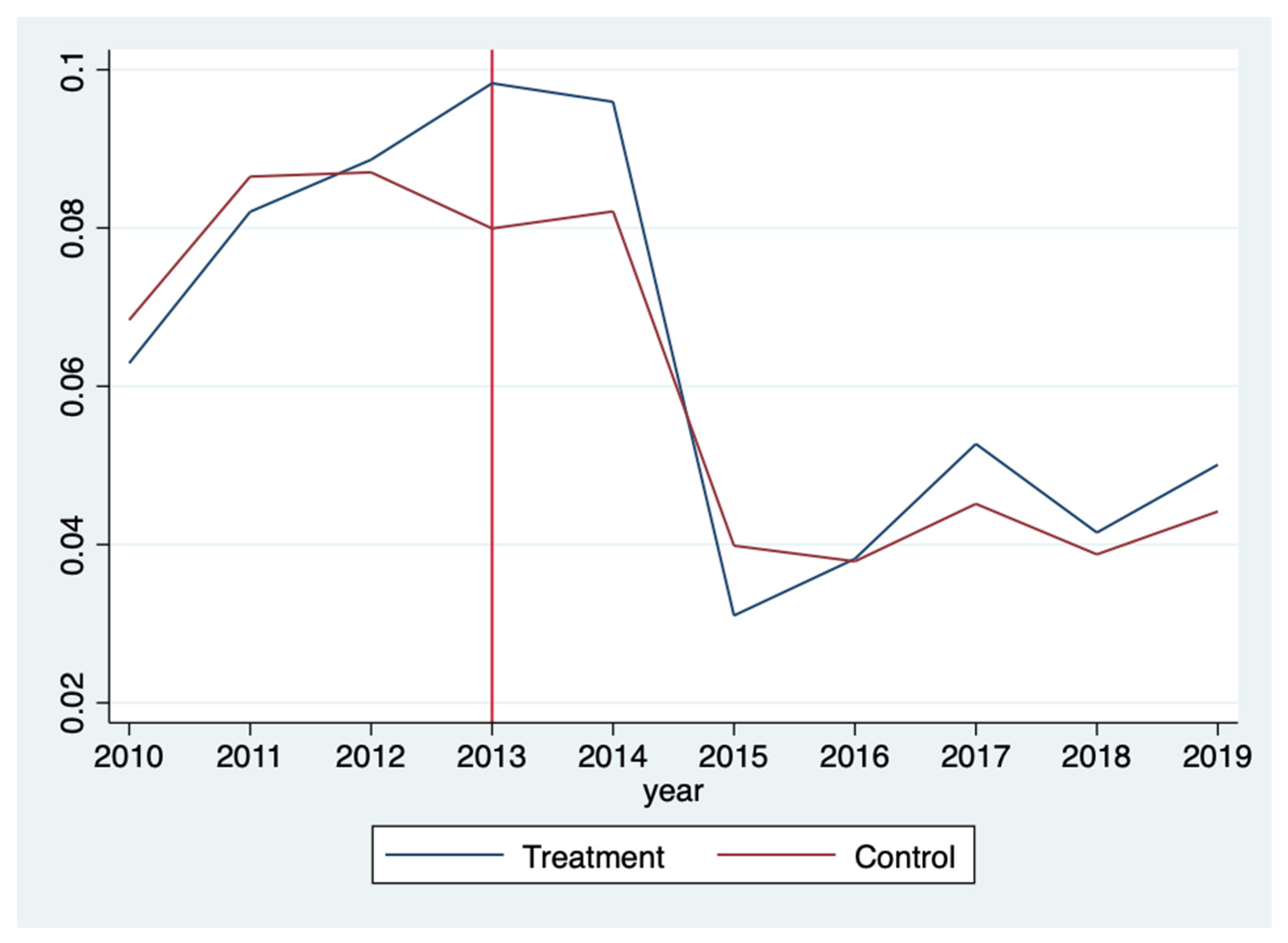
5.2. Placebo Test

As a robustness check, I also repeated the analysis above for the variable indicating the purchase of other “non-major” appliances such as “TVs, tape recorders, video recorders, musical instruments, computers, cameras and the like” as outlined in the questionnaire of RLMS-HSE [29]. If the increased propensity to purchase major electrical appliances in treatment regions is indeed attributed to the introduction of the IBR tariff scheme, then we should not observe the same effect for the purchase of other “non-major” appliances in treatment regions as they are usually not that energy-intensive.

Indeed, from Figure 3 and

Table 6. Unconditional DiD Estimates for Propensity to Purchase Non-Major appliances.

	Pre-Period	Post-Period	Difference (Post-Pre)
T = 1	0.0778	0.0586	−0.0192
T = 0	0.081	0.053	−0.028
Diff-in-Diff			0.0088 (0.0077)

Robust standard error in parentheses; * p < 0.1, ** p < 0.05, *** p < 0.01; Source: Author’s own calculations.

below, we cannot observe any significant relationship either graphically or in the DID specification. However, we can observe a sharp decline both in the treatment and control regions of the propensity to purchase non-major electrical appliances in 2015. Again, we can attribute this to the effect of the economic sanctions imposed by the international community at the end of 2014.

In the case of non-major appliances, the decline is much more pronounced, with about a four-percentage point decrease in the control regions and more than a six-percentage point decrease in the treatment regions. We can observe that the purchase of non-major appliances in treatment regions fell by about 60% in 2015, while it increased in the case of major appliances by about 15% in the same year.

5.3. Fixed Effects Estimation Results

Next, I estimated the DiD model for major electrical appliances using a fixed-effects model to observe if the effect of IBR on the propensity to purchase major electrical appliances was robust to the inclusion of the household and year fixed effects, as well as some additional time-varying covariates. I included the total household income, the total amount of discounts and subsidies received by the household for utilities, the average price for the electricity, and household size as additional covariates.

Column 1 of

Table 7. Results.

	(1)	(2)	(3)	(4)
	FE	FE _Matched	FE _2SLS	FE_2SLS _Matched
DiD	0.0224 *	0.0224 *	0.0228 *	0.0229 *
	(0.013)	(0.013)	(0.013)	(0.013)
lnPrice	−0.0111	−0.0120	−0.0128	−0.0137
	(0.023)	(0.023)	(0.023)	(0.023)
lnIncome	0.0463 ***	0.0471 ***	0.0463 ***	0.0471 ***
	(0.004)	(0.004)	(0.004)	(0.004)
lnDiscounts	0.0008	0.0007	0.0008	0.0007
	(0.001)	(0.001)	(0.001)	(0.001)
lnSubsidies	0.0014 **	0.0013 *	0.0014 **	0.0013 *
	(0.001)	(0.001)	(0.001)	(0.001)
HHsize	0.0032	0.0024	0.0032	0.0024
	(0.003)	(0.003)	(0.003)	(0.003)
year11	0.0066	0.0072	0.0067	0.0073
	(0.006)	(0.006)	(0.006)	(0.006)
year12	0.0104 *	0.0084	0.0104 *	0.0085
	(0.006)	(0.006)	(0.006)	(0.006)
year13	0.0159 **	0.0152 **	0.0160 **	0.0153 **
	(0.006)	(0.007)	(0.006)	(0.007)
year14	0.0084	0.0076	0.0084	0.0077
	(0.006)	(0.007)	(0.006)	(0.007)
year15	−0.0209 ***	−0.0209 ***	−0.0208 ***	−0.0208 ***
	(0.006)	(0.006)	(0.006)	(0.006)
year16	−0.0122 **	−0.0125 **	−0.0122 **	−0.0125 **
	(0.006)	(0.006)	(0.006)	(0.006)
year17	−0.0029	−0.0023	−0.0031	−0.0025
	(0.006)	(0.007)	(0.006)	(0.007)
year18	−0.0103	−0.0115	−0.0105	−0.0118 *
	(0.007)	(0.007)	(0.007)	(0.007)
year19	0.0015	0.0014	0.0012	0.0010
	(0.008)	(0.008)	(0.008)	(0.008)
_cons	−0.3586 **	−0.3607 **
	(0.148)	(0.150)
N	53,040	51,608	53,040	51,608
adj. R2	0.02	0.02	0.02	0.02
F	15.3988	14.9204	15.4031	14.9256
p	0.0000	0.0000	0.0000	0.0000

Robust standard errors in parentheses; * p < 0.1, ** p < 0.05, *** p < 0.01; Source: Author’s own calculations.

presents the results of the fixed effect estimations obtained via LPM. I then repeated the same estimations (Column 2 of Table 7) by applying the full block-tariff schedule for electricity as an instrument for the average electricity price to address any potential endogeneity concerns resulting from a nonlinear electricity tariff schedule. Column 3 and Column 4 repeat the aforementioned estimations but with the application of the coarsened exact matching (cem) technique prior.

Across models, we can see that there is some evidence of the relationship between the IBR pricing scheme and the propensity to buy major electrical home appliances. The DID estimator characterised by the interaction of the binary treatment indicator with the binary indicator for the post-treatment period is positive and statistically significant, both in ordinary FE specification and when instrumenting the price of electricity with a full block-tariff schedule.

Depending on the specification, the coefficient on the DiD estimated via LPM is between 0.0224 and 0.0229. This implies that, depending on the specification, the propensity to purchase major electrical appliances is 2.24–2.29 percentage points (or more than 20%) higher, on average, in the regions with the IBR tariff scheme. The estimates are mostly in line with the unconditional DID estimate reported in Table 5, although the statistical significance falls from 5% to 10%. Taking into account that in the FE specifications, we control both for observed and unobserved time-invariant factors, along with some additional time-varying covariates included in the model, this fall in significance is not surprising.

Instrumenting for the average prices of electricity with the full block-tariff schedule does not alter the estimation results. The coefficients estimated by the FE are practically identical to the estimators in the 2SLS context, which mitigates the potential endogeneity concerns in our model specifications (The first stage regression results are available in Appendix B. Please note that due to the block cut-offs being household and dwelling specific, there are a total of 35 different tier cut-offs).

Regressions based on coarsened exact matching (cem) procedure perform reasonably well in our specification. We “coarse” our continuous variables (square footage of the dwelling, size of the household, and household income) into ten quantiles and match the treatment and control units according to the quantiles they are located in and the binary household characteristics: single-family or multi-apartment, location (urban, rural), and whether the household is connected to the central delivery of hot water, and central heating.

Applying the matching prior to the estimation of DID, however, also did not produce any significant difference in estimation results. Although we observed some improvement in the overall balance of covariates between the IBR and non-IBR households, given by the multivariate L1 (L1 is a comprehensive imbalance measure given by: $L_{1 }\left(f,g\right)=\frac{1}{2}{\displaystyle \sum }_{l_1\dots l_k}| f{ }_{l_1\dots l_k}-g_{ l_1\dots l_k}|$ where $f{ }_{l_1\dots l_k}$ and $g_{ l_1\dots l_k}$ are the k-dimensional relative frequencies for the treated and control groups, respectively, calculated from the cross-tabulation of the discretised (coarsened) covariates) distance statistics [39], the regression coefficients were close to their unmatched counterparts.

First, the L1 distance statistics were calculated for the unmatched data, which would then serve as a point of comparison (a baseline reference) for the matched data. If L1 statistics were closer to zero (one indicating a perfect imbalance, while zero indicating a perfect balance of covariates) on a match data, as compared to its unmatched counterpart, then we could argue that there was an improvement in the balance of covariates across the treatment and control groups after the matching procedure.

In our case, the multivariate L1 distance statistics for the unmatched data was 0.636, while for the matched data, it was equal to 0.57, indicating an overall improvement in the balance between the two groups (It should be noted that the absolute values of the L1 statistics mean less than comparisons between the matching solutions. In this sense, the L1 statistics work for imbalance as R-squared works for the model fit).

By examining the covariates across all specifications, I found no evidence of the effect of the level of the price of electricity (as opposed to its structure represented by the DID term) on the propensity to purchase electrical appliances by households. The coefficient on the average price was statistically insignificant. This finding is in accord with the recent study of Jacobsen (2015), who also concluded that the actual level of the electricity prices do not affect the purchasing decision of the Energy Start certified home appliances in the US.

The effect of the total household income, on the other hand, is positive and statistically significant at 1%. The estimation results suggest that a one percent increase in income results in about half a percent increase in the probability of purchasing major electrical appliances (the elasticity in the linear-logarithmic specification is obtained by: b*(1/Y)).

Both household size and the discounts for the utilities have a statistically insignificant association with the propensity to purchase electrical appliances. Subsidies have a positive and statistically significant association, although the coefficient is small in size, which suggests that the relationship is economically insignificant.

6. Conclusions

By using the variation resulting from an implementation of the IBR tariff for residential electricity in three experimental regions in Russia and household panel data, I examined the relationship between the IBR pricing and the propensity of the households to purchase major electrical appliances. To the best of my knowledge, this is the first paper that has combined household-level panel data with a natural experiment to study the relationship between IBR pricing and the propensity of households to purchase electrical appliances. I found evidence that in the regions where the IBR pricing was implemented, the households’ tendency to purchase the major electrical appliances increased by more than 20% (two percentage points). This result is robust both in standard fixed effects regression as well as when instrumenting for the electricity prices with a full block-tariff schedule.

It should be noted, however, that from the data, I could not observe the actual energy efficiency rating of any of the purchased appliances. As such, I am unable to comment on whether consumers respond to IBR pricing by purchasing more energy-efficient appliances. I am also unable to comment on how IBR pricing affects investment in other types of household products, such as more efficient light bulbs, furnaces, or insulation.

However, taking into account the robust trend of newer appliances being more energy-efficient, I can suggest that consumers that purchase new electrical appliances are also purchasing more energy-efficient appliances. If this proposition holds, the results of this paper can suggest that price-based energy policies are an effective tool not only in shaping the behaviour of the household but also in shaping the households’ behaviour towards higher energy efficiency, which is considered one of the lowest-cost opportunities for reducing carbon emissions.