Article

Fundamentals of the Thermal Analysis of Complex Arrangements of Underground Heat Sources

1
Faculty for Engineering Sciences, Institute for Energy-Transport and Storage (ETS), and Head of BCC Cable Consulting, University of Duisburg-Essen, D47495 Rheinberg, Germany
2
Faculty of Electrotechnics, Electronics and Automation, Lodz University of Technology, 90-924 Lodz, Poland
*
Author to whom correspondence should be addressed.
Energies 2021, 14(20), 6813; https://doi.org/10.3390/en14206813
Submission received: 16 September 2021 / Revised: 4 October 2021 / Accepted: 7 October 2021 / Published: 18 October 2021
(This article belongs to the Topic Power Distribution Systems)

Abstract

:
This paper introduces a new analytical method for the 3-dimensional analysis of heat sources installed underground. Such sources include primarily electric power cables and steam pipes in urban areas. For complex arrangements of the heat sources, the heat transfer and cable rating calculations require the application of numerical methods, which call for high level of expertise and are generally difficult to use. The computational algorithm presented in this paper uses a point sources approach and is an extension of the work published by the authors based on line source modeling, with the goal of simplifying the numerical calculations. The proposed approach is applicable for all heat sources, which are directly buried in a uniform or a partially dried out soil. The method is illustrated by several numerical examples. These examples are used for comparison with the existing standard approach.

1. Introduction

Knowledge of the current carrying capacity of electric power cables, or ampacity (or rating) for short, is needed when the cable system is designed and it is an important parameter during its operation. Cable ampacity is dependent on its construction, laying conditions and the duty cycle. The heat generated by the loaded cables is dispersed in the surrounding environment. Thus, the analysis involves two types of calculations: (1) evaluation of the heat generated inside the cables, and (2) heat transfer through the cable components and the surrounding soil.
The heat is generated by the load current in the conductor and, for alternating currents, by the induced currents in other metallic parts of the cable. Additionally, the alternating voltage generates dielectric losses in the insulation. The heat transfer inside and outside the cable is described by partial differential equations of heat conduction, which are in principle nonlinear, because of the temperature-dependency of the losses. For simple cable arrangements, these equations can be solved analytically with some simplifications. For such cases, the generation of the heat and the heat transfer equations are described in the national and international standards. Perhaps the most widely used standards are those published by the International Electrotechnical Commission (IEC) [1,2,3]. The derivation of the equations found in the IEC standards, as well as the long history of their development, can be found in [4].
However, in many cities around the world, cable infrastructure can be very complex, especially in the vicinity of substations, and in those situations, only numerical approaches are available for performing ampacity studies. The finite element method (FEM) or the finite difference approach (FDA) are the solutions of choice, with the former being the most widely used.
In recent years FEM has been used to analyze cable losses, with several different software packages, in 2D [5] and in 3D [6]. The method has also been used to combine electromagnetic models with thermal conduction, in 2D [7] and 3D [8]. FEM has been used to study convection and radiation heat transfer in risers (J/I-tubes) [9] and horizontal pipes (HDD) [10] with computational fluid dynamics and with heat transfer coefficients [11].
However, computer programs based on applying the finite element method to solve partial differential equations describing heat generation and heat transfer of the power cables require great skill in their application and are generally difficult to use. The first analytical description was developed in [12], in which straight sections of the cables are represented as line sources with finite lengths. Attempts to address cables crossing other heat sources for rectilinear cables were described in [13,14,15]. The concept of finite line sources in [12] was recently used to calculate the thermal fields of such complicated cable structures, taking the longitudinal heat flows along the cable conductors into account [16].
However, during some numerical applications, several important disadvantages of the method of finite line sources became evident. First, the numerical handling of the line sources, which result from subdividing straight cable sections into subsections, is elaborate and somewhat error-prone. The same holds true for the analysis of the finite line sources (the number of which may be more than 10,000 per cable), where for each of them, the coordinate system must be defined to consider each field point by means of a transformation of the coordinates. Moreover, for sloped cable sections (where the laying depth is changing), no representation by line sources is known. Furthermore, a severe disadvantage is that no formulations of the transient behavior of finite line sources are known, so that an analysis of such arrangements for time-dependent loads is not possible.
To overcome these problems, a new model is presented in this paper. This model uses point sources instead of line sources. The method can be abbreviated as PSM, referring to the point sources method. As shown below, it is easy to use and is applicable to all possible configurations of buried heat sources. The method not only enables steady-state analysis, taking into account the drying-out of the soil and/or longitudinal heat flows, but also allows the calculation of the transient thermal behavior with time-varying heat inputs.

2. Basic Principles

The main idea is to subdivide all heat sources in a given installation into short sections (normally of equal length of, e.g., 0.01 m), which will be represented as point sources with the emission of the local losses W.

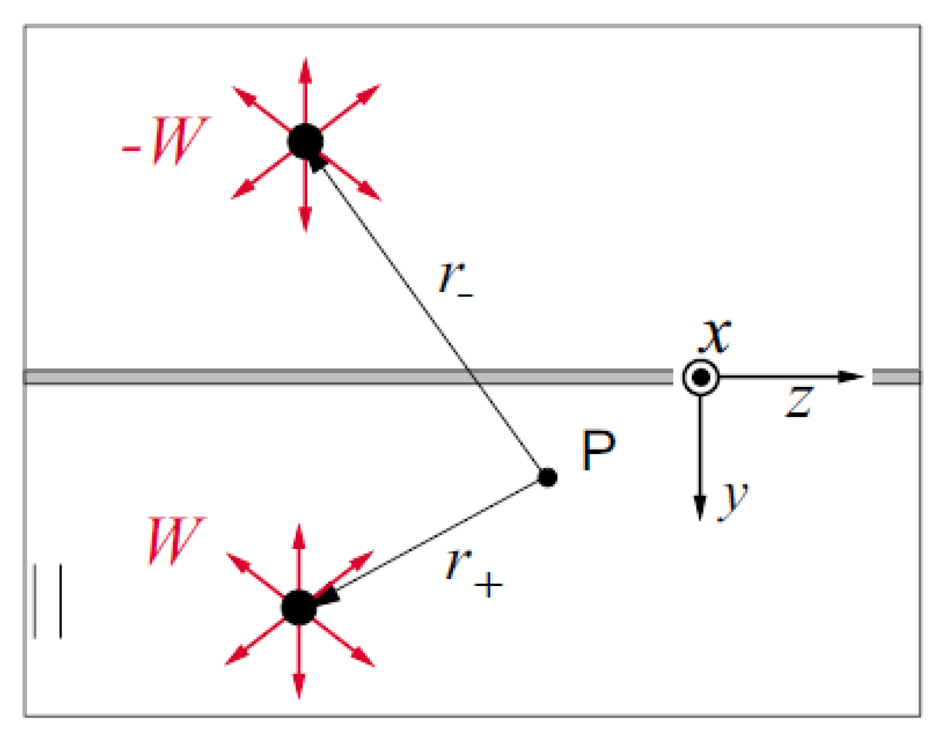
2.1. Steady-State Temperatures

The steady-state temperature rise Δθ caused by a point source is given by:
Δ θ = W 4 π λ 1 r + c
where
  • r—distance between a point source (with losses W) and the considered point,
  • λ—thermal conductivity of the soil, and
  • c—constant.
Similar to the Kennelly formula, which is normally used by cable engineers for long, straight cables and is based on an infinite line source, we consider the influence of the isothermal soil surface by reflecting the point source and weighting it with the losses –W, as illustrated in in Figure 1.
Thus, we can obtain the steady-state temperature rise Δθ caused by a point source in the soil:
Δ θ = W 4 π λ ( 1 r + 1 r )
where r + ,   r _ are the distances between the source (with losses W) and the reflected source (with losses —W) in relation to the considered point.
Note that summarizing an infinite number of point sources by means of (2), along an infinite line (which is also reflected at the soil surface) leads to the model shown in Figure 2 and (for constant losses) to the well-known Kennelly equation for the temperature rise caused by an infinite line source in the soil:
Δ θ = Δ l 4 π λ i = 1 N W [ z ( i ) ] ( 1 r + , i 1 r , i ) 1 4 π λ ( 1 r + 1 r ) W ( z ) d z = 1 4 π λ l n r r +
with the distances between the considered point P (xP, yP, zP) and the point source (x1, y1, z1) expressed as:
r + = ( x p x 1 ) 2 + ( y p y 1 ) 2 + ( z p z 1 ) 2 ,   r = ( x p x 1 ) 2 + ( y p + y 1 ) 2 + ( z p z 1 ) 2
In this paper, the losses per unit length (p.u.l.) will be denoted by W′ and the losses of a point source by W. The notation z′ pertains to the local coordinate system associated with the considered heat source.
From the above developments, we have the possibility of describing any section of a heat source—straight or curved—through the superposition of point sources with constant or varying losses. For this purpose, the considered heat source section must be subdivided into small sections of equal lengths. The next question is what the maximum length of these sections should be so that an approximate representation by the point sources works with a sufficient accuracy. To examine this question, consider Figure 3, which shows the temperature rise caused by a line source extending from z′ = −10 m to z′ = +10 m and the losses (p.u.l.) of W = 100 W/m at the distance xP from the axis of the line source (at z′ = 0). The line source is represented by the point sources of length Δl and losses of W   Δ l The depth of laying is y = 2.0 m.
The dotted red line shows the exact solutions, resulting from (3), for different points (xP). We can observe that even for the very small lengths Δl, there is a deviation from the exact solution. This deviation is a result of the limited length of the examined line source (i.e., from the “missing ends”). This topic will be discussed later in the text.
If the value of xP is interpreted as half of the cable or heat pipe diameter (assuming that the conductor’s center is on the z-axis), Figure 3a,b describe cables/pipes with diameters between 20 and 100 mm. It can be concluded that even for the very small cables, the length of Δl = 0.01 m = 1 cm will be sufficient.
The remaining deviation (as compared with the infinite line source) can be explained by examining Figure 4. In the right-hand part of this figure, cable/pipe is represented by a semi-infinite line source, which again is represented by “point sources” of length Δl. Obviously, for calculating the temperature rise ΔθP at the point at a distance xP from the heat source axis and in a distance Δz to the end of the section, the deviation of ΔθP from the exact solution for an infinite line source will increase with decreasing distance Δz, caused by the left-hand “missing end”.
To examine this effect further, let us consider a heat source that is 130 m long. The heat source is represented by point sources (with Δl = 0.01 m) and we are interested in the temperature at the same distances xp from the z-axis, as in Figure 4. Computed temperature rises are shown in Figure 5 as a function of Δz (keep in mind that in Figure 3 we have a distance of ±10 m to both ends, which will double the deviation). From Figure 5, it can be concluded that if a point of interest is in the range of 10…20 m remote from the line source end, the calculation errors caused by the missing cable ends will become negligible.
Thus, we have found an algorithm which can easily be applied to all geometries of a heat source run. A precondition of the calculation is a subdivision of the run into small sections of equal length (of, e.g., 0.01 m) and to define the coordinates of the center points of these subsections, which are treated as point sources. Moreover, the emitted losses (p.u.l.) W′ are to be defined first, which can consequently be locally handled in a function of temperature. This will be discussed in detail in the following chapters.

2.2. Transient Temperatures

A point source with a loss step ΔW at the time t = 0 will cause the following temperature rise in a considered point at the distance r [17]:
Δ θ ( t ) = Δ W 4 π λ 1 r erfc ( r 4 δ t )
with δ thermal diffusivity of the soil. As shown in [3], this variable can be approximated by means of the following equation:
δ = 4.68 × 10 7 [ λ W / ( Km ) ] 0.8 m 2 s
The error function erf(x) and its complementary function erfc(x) are defined by:
erf ( x ) = 2 π 0 x e u 2 d u                   erfc ( x ) = 1 erf ( x )
Following [18], a numerical solution can be achieved by:
erfc ( x ) = [ 1 + a 1 x + a 2 x 2 + a 3 x 3 + a 4 x 4 + a 5 x 5 + a 6 x 6 ] 16 + ϵ
with the maximum absolute value of the error of | ϵ | < 3.10 7 . The coefficients ai are equal to:
[0.0705230784, 0.0422820123, 0.0092705272, 0.0001520143, 0.0002765672, 0.0000430638]
Since erfc ( 0 ) = 1 , we see from (5) that for large values of time t and/or for large distances r, the solution approaches the steady-state description of (1).
Reflecting the point source at the soil surface again, as was done for the steady-state analysis, and superimposing all N point sources along a line section, gives a temperature rise of:
Δ θ ( t ) = Δ l 4 π λ i = 1 N Δ W [ z ( i ) ] ( 1 r + , i e r f c ( r + , i 4 δ ( t t i ) ) 1 r , i e r f c ( r , i 4 δ ( t t i ) ) )
where the point sources i at places z′ = i Δz have loss steps Δ W i at times ti.
A summation in (9) over an infinite number of point sources along an infinite line (which is also reflected at the soil surface) leads to the model of Figure 2 and (for constant losses) to the well-known equation for the transient temperature rise caused by an infinite line source with the loss step (p.u.l.) ΔW′:
Δ θ ( t ) = Δ W 4 π λ [ E 1 ( r 2 4 δ t ) E 1 ( r 2 4 δ t ) ]
with the exponential-integral-function E1:
E 1 ( x ) = 2 π x e u u d u
Figure 6 shows the correspondence of the solutions (10) for the line source (red lines) and (9) for the point sources (green lines). It shows the temperature rise at a point at the distance Δy below the line caused by a line of point sources at the depth of y = 2.0 m and with the end coordinates of ±30 m. We consider a loss step at t = 0 in all point sources with ΔW′ = 100 W/m. It can be seen that both solutions are practically identical.

3. Some Basic Examples

In this chapter, some basic examples of the application of the calculation model will be presented.

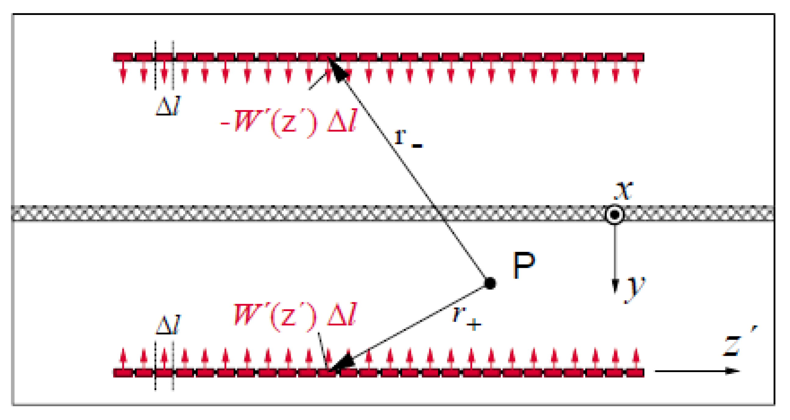
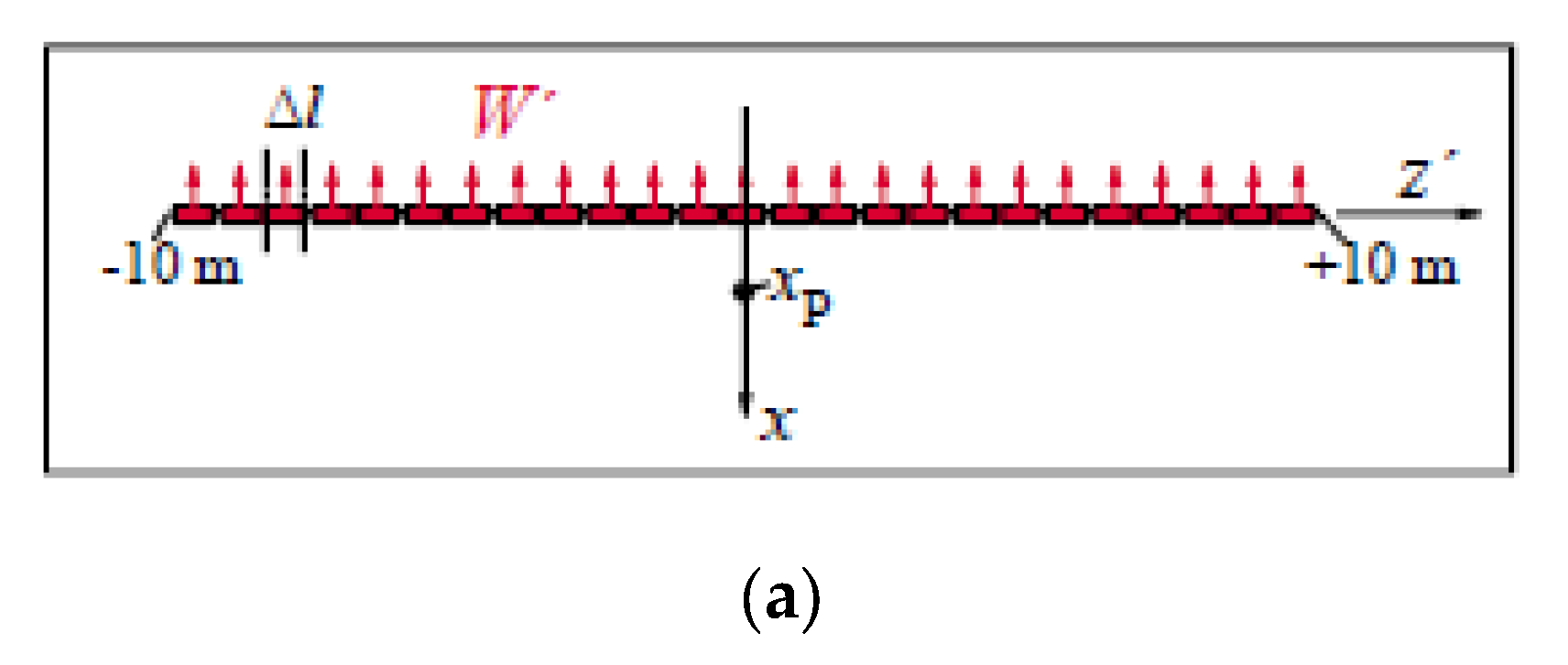
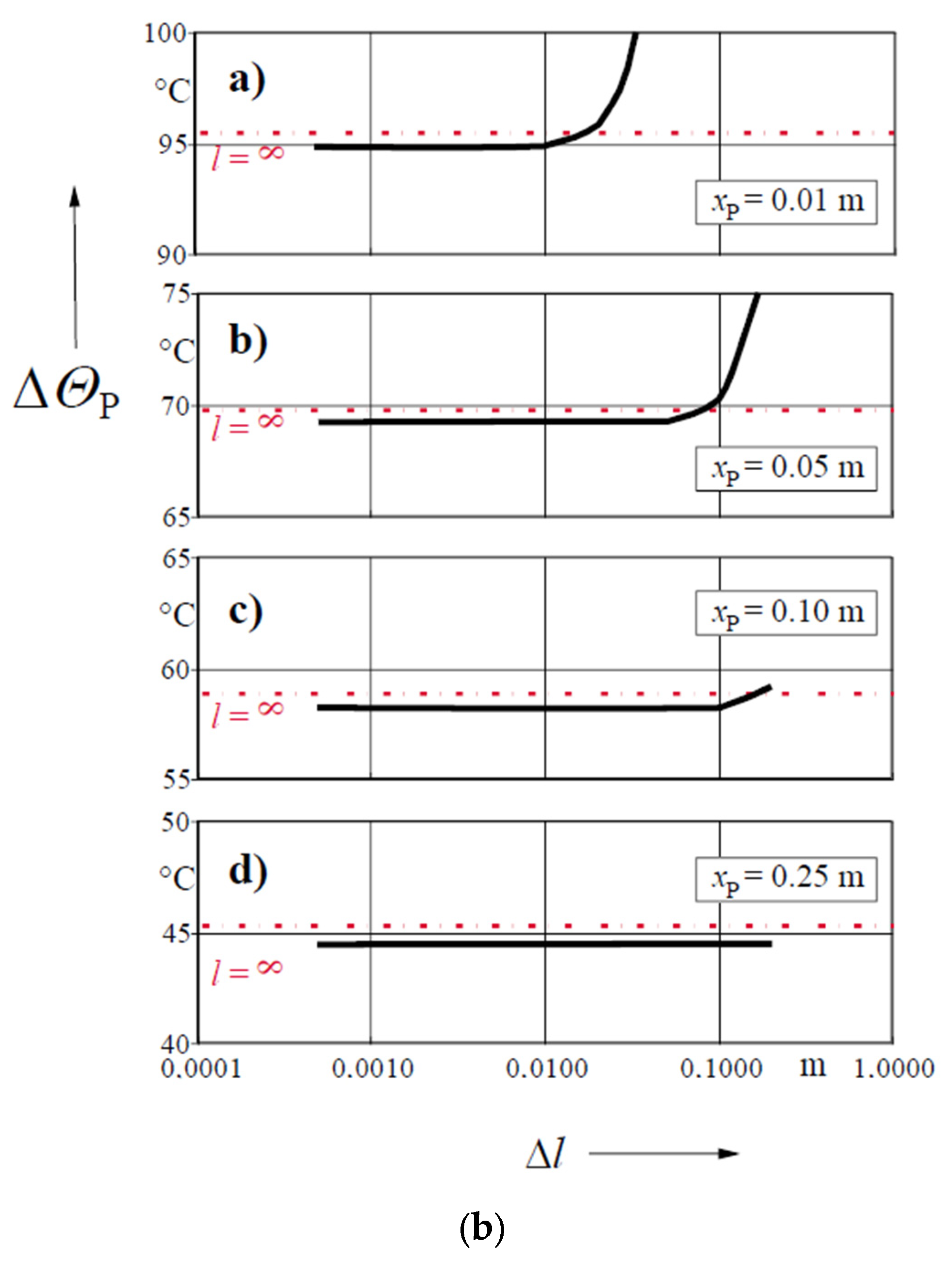
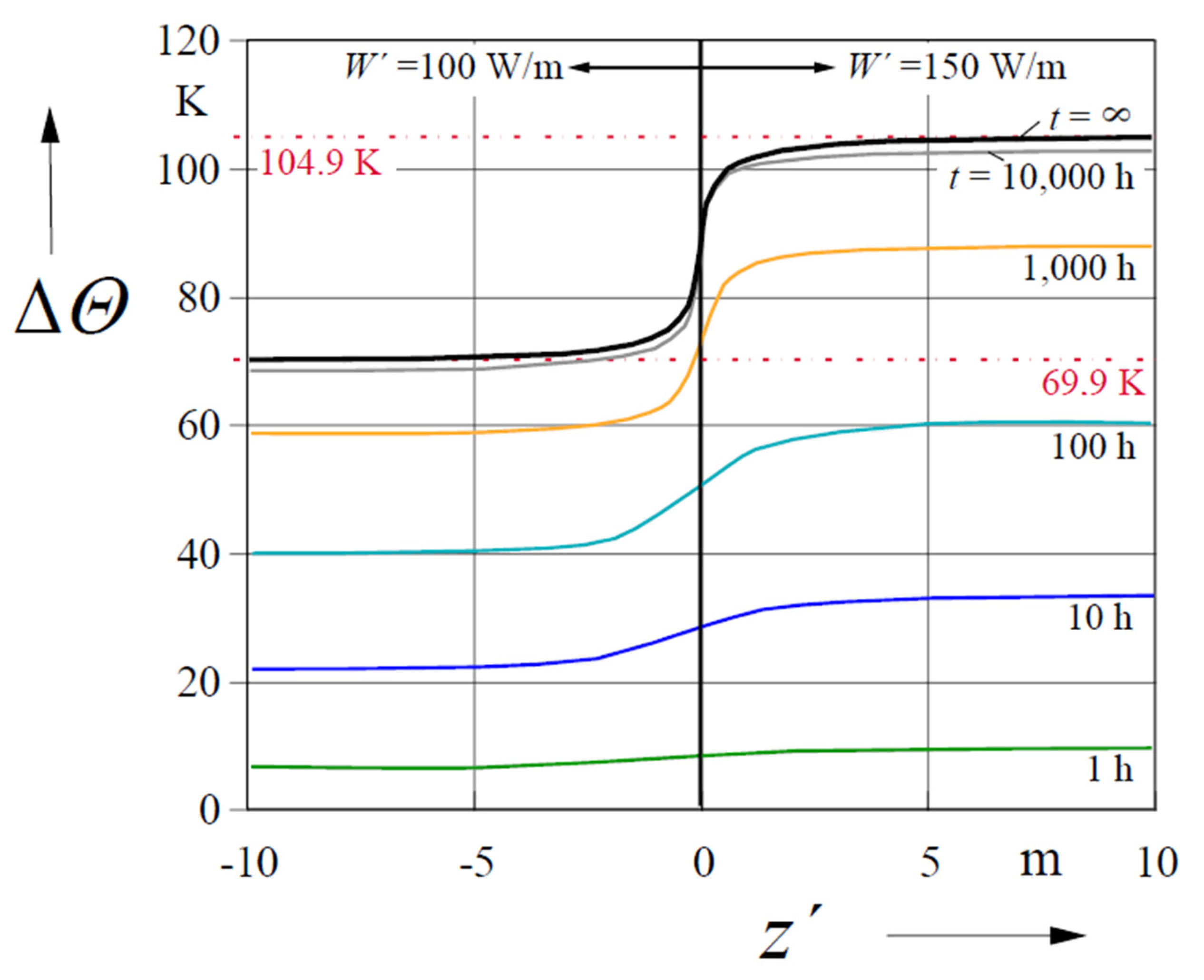
3.1. Line Source with Locally Varying Losses

Consider a line source shown in Figure 7 with z′ = −30 … + 30 m and losses (p.u.l.) of 100 W/m for the section z′ = −30 …0 m and of 150 W/m for z′ = 0 …30 m (the technical background may be a cable with a changing cross section or a steam pipe with a changing temperature at z′ = 0 m). These losses arise as power steps at t = 0.
The thermal response at a point with a distance of Δy = 0.05 m below the line source as a function of the axial coordinate z′, for different instants of time is shown in Figure 8. The red chain of dotted lines indicate the stationary solutions calculated separately by the line sources model (3) for the two loss values. It can be seen in Figure 8, that the transient run for large times (black line) calculated with an application of 2 × 6000 point sources correspond—at a sufficient distance from the transition point z ′= 0 m—completely with the steady-state solutions of the infinite line sources.

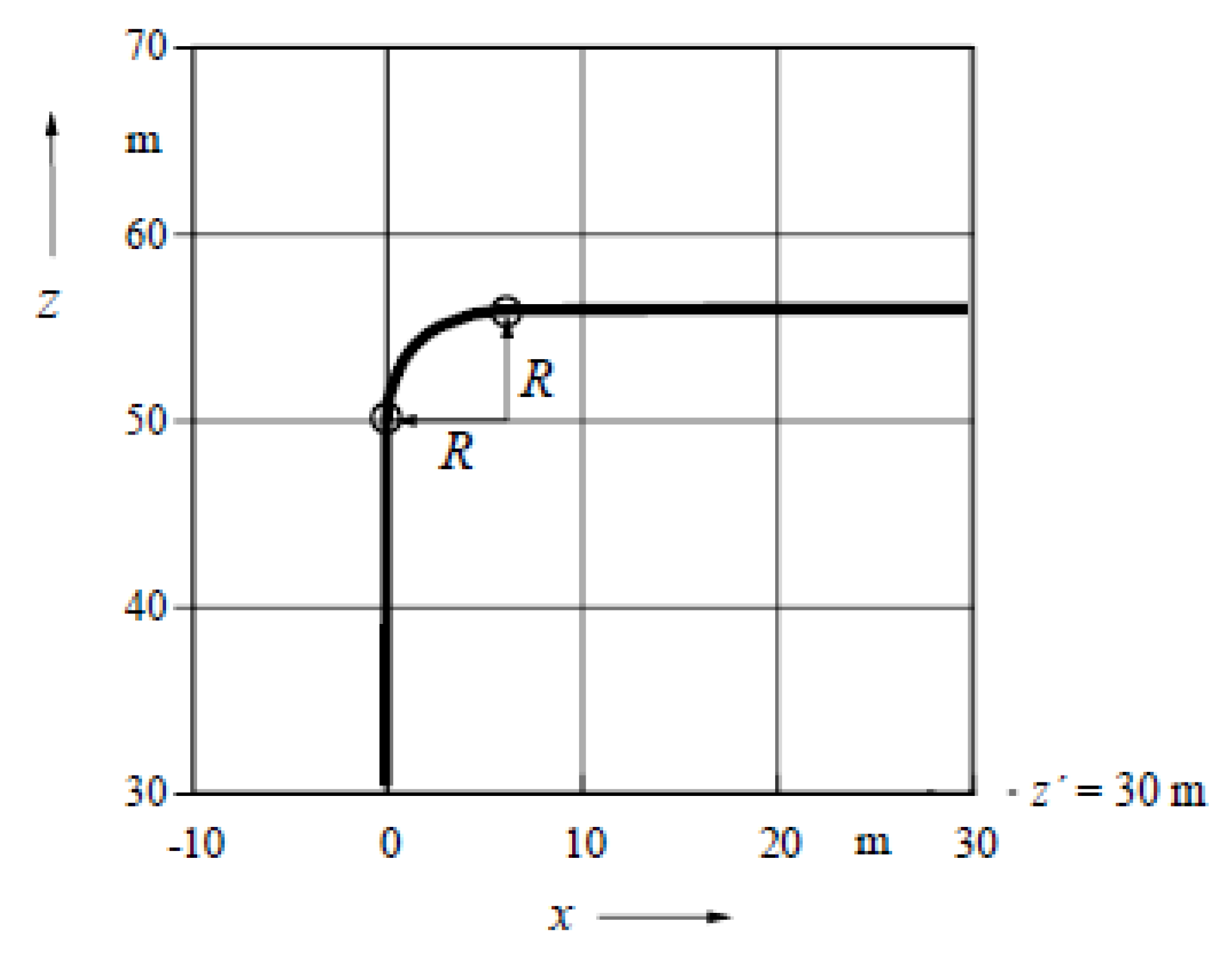
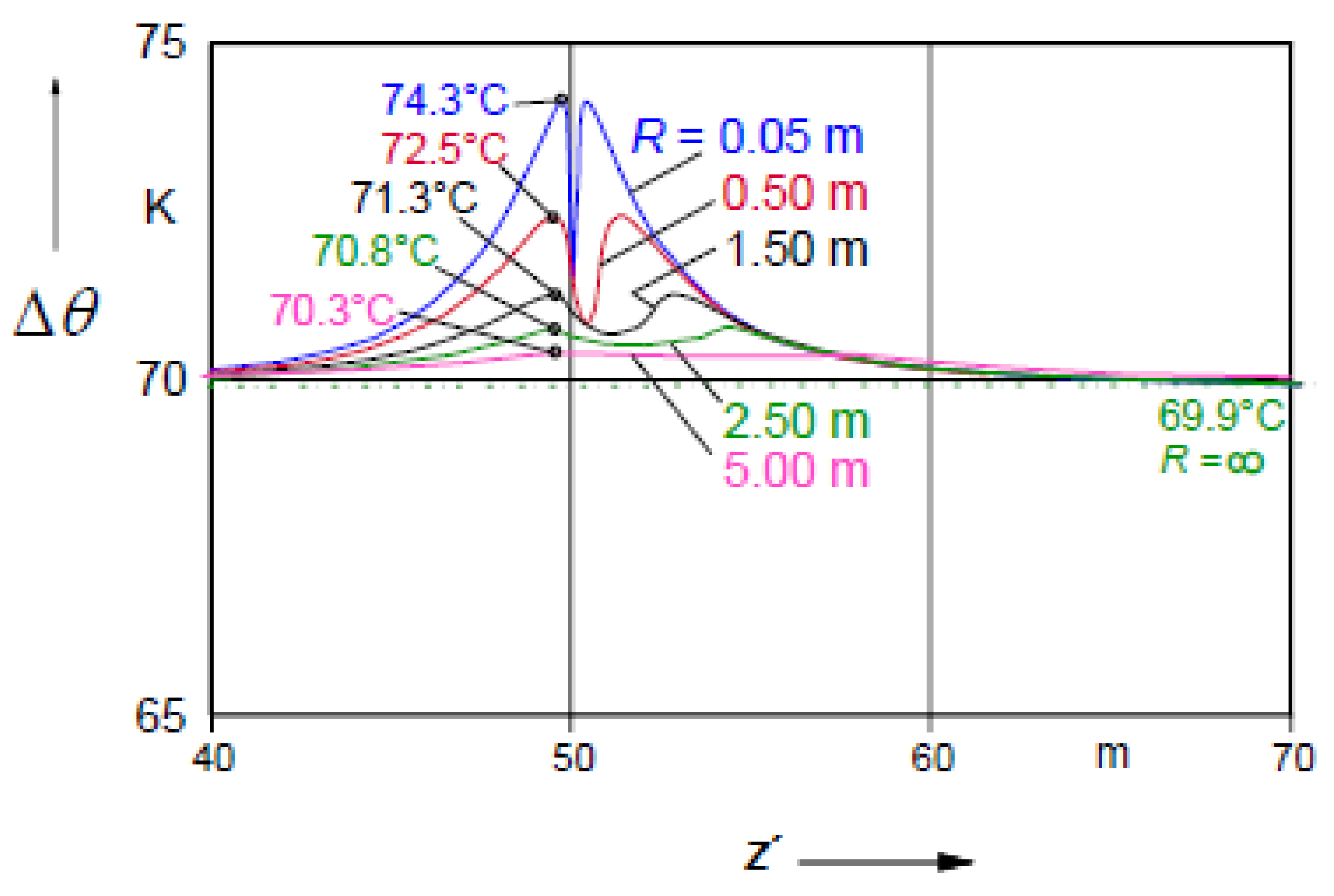
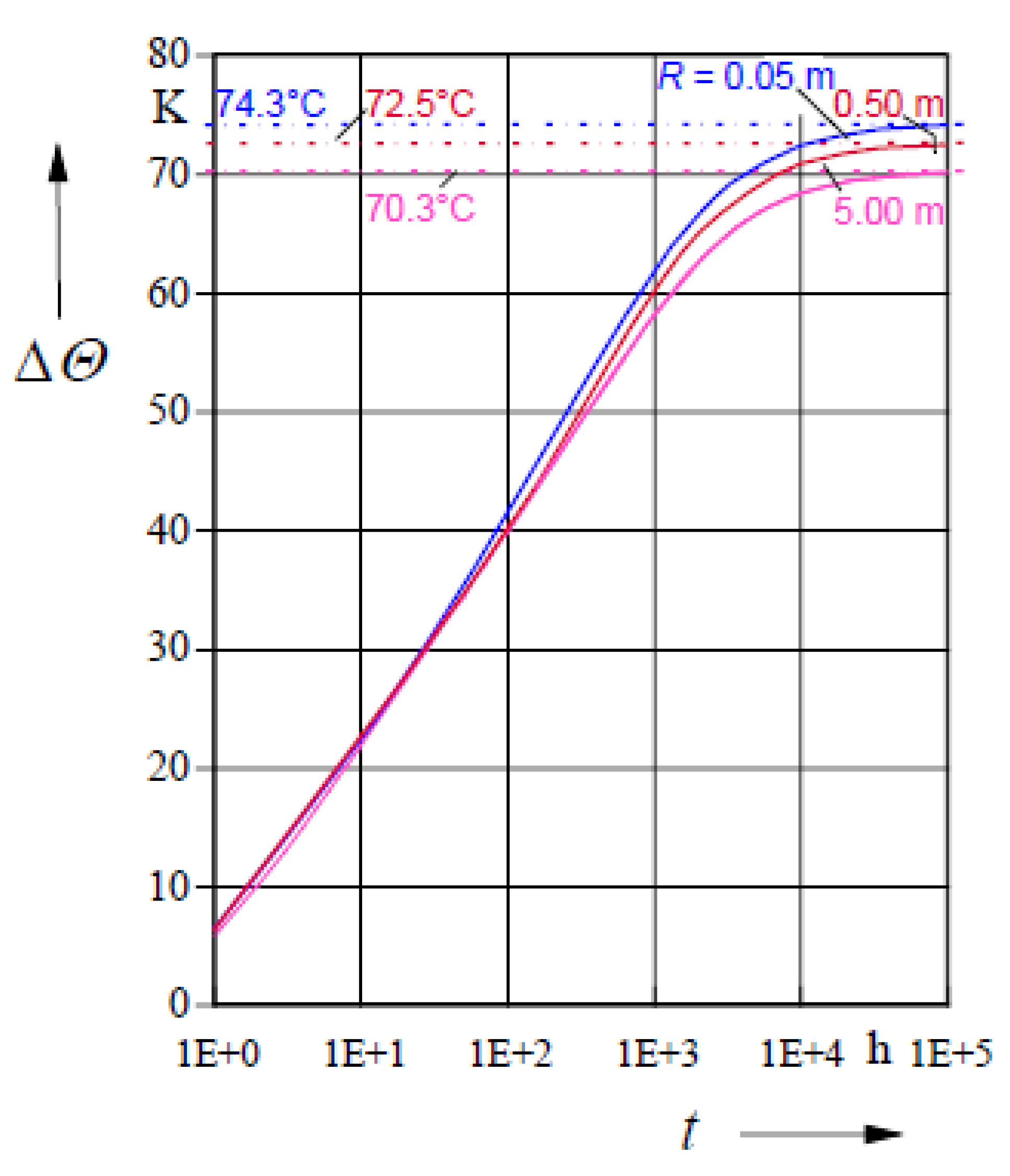
3.2. Line Source with a 90° Bend

In the following, the thermal behavior of a line source with a 90° bend will be discussed, as shown in Figure 9. Such situations often arise in practice but there are no analytical tools to handle them. Figure 9 shows the geometry of the bend with the radius R. The line has a depth of y = 2.0 m and is represented along its axis (z′ = 0…100 m) by point sources, again defined by a length of Δl = 0.01 m, a depth of y = 2.0 m and a thermal conductivity of the soil of λ = 1.0 W/(K m).
Figure 10 shows the temperature rises along the bend, 0.05 m below (y = 2.05 m) the line source, as a function of the axial coordinate z′ with the bending radius R as a parameter. With increasing z′, the bend begins at z′ = 50.0 m (see Figure 9).
Figure 10 illustrates that at both sides of the bend we have the maximum values of the temperature rise, which are dependent on the bending radius. A minimum value of the temperature rise appears in the middle of the bend, but this remains higher than the compared temperature rise of a straight line without a bend (69.9 K). This value is again approached by all the characteristic lines for small and large values of z′.
For the points with temperature maxima, which are marked in Figure 9 by small circles, the transient temperature rises are calculated, using (7), for a loss step (p.u.l.) of W′ = 100 W/m at t = 0. The results are shown in Figure 11, in which the temperature runs are well approaching the stationary values of Figure 10.
Typical minimal bending radii Rmin of power cables are 15–25 times the cable radius. This means that for a small medium voltage cable with a diameter, e.g., of 30 mm: Rmin = 0.45…0.75 m, whereas an extra-high-voltage cable with a diameter of, e.g., 140 mm, has Rmin = 2.1…3.5 m. From Figure 10, we can conclude that in the first example the temperature rise caused by the bend is appreciable (>5%), whereas in the second example, it is nearly negligible.

4. Temperature and Rating Analysis of a Complicated Cable Route

The foregoing basic explanations of the new method for determining the temperature rise in the soil surrounding heat sources can be applied for the temperature and rating analysis of complicated cable arrangements.

4.1. Steady State, without Longitudinal Heat Fluxes

For determining the steady-state conductor temperature of a cable, the normal relations of the IEC Standard 60287 [1,2] can be used, but applied to a predefined section i s of cable i. For a single-core cable i, installed in a group of N cables, we obtain the conductor temperature in section i s by superposing the temperature rises caused by all sections j s = 1 , N s j in all cables 1…N:
θ c , i , i s = δ i j W c , i , i s ( T c a b , i + T 4 , i ) + j = 1 N j s = 1 N s , j W j s T 4 , j s , i s + Δ θ d , i s + θ a m b
here:
T c a b , i = T 1 , i + ( 1 + λ 1 ) T 2 , i + ( 1 + λ 1 + λ 2 ) T 3 , i
  • Δ θ d , i s = temperature rise of conductor section is because of the dielectric losses of cable, (K)
  • T1, T2, T3 = thermal resistance of the insulation, armor bedding and the jacket, respectively, (K.m/W).
  • λ1, λ2 = sheath and armor loss factors, respectively
  • W j s = total losses of section js in cable j, (W).
  • δi,j is the Kronecker-symbol with δi,j = 1 for i = j and δi,j = 0 otherwise.
  • T 4 , j s ,     i s is the thermal resistance between section js of cable j and section is of cable, (K·m/W). Following (3), with Ns,j sectors (i.e., point sources) of the influencing cable j, we have:
    T 4 , j s , i s = Δ l 4 π λ l = 1 N s , j ( 1 r + j s , i s 1 r j s , i s )
    where the radii r+ and r-- are the distances between the considered section is and the influencing point source js (and its image source, respectively).
We will now discuss a practical example, shown in Figure 12, which illustrates a crossing area with nine 220-kV-XLPE-cables (3 × 3 × 1 × 2500 mm2 copper; 60 Hz, the cable construction is described in detail in [16]). The laying depth of all cables is y = 2.0 m for z < 13.0 m. With increasing z, the crossing cables 4…9 are rising between z = 13.0 …15.0 m from y = 2.0 m to y = 1.4 m. The distance of the axes in all systems is 1.0 m, and the radius of the inner cables in all bends is 2.0 m. The currents of all cables are given as 1600 A. The ambient temperature is 15 °C, and a homogeneous soil with a thermal conductivity of 1.0 W/(K m) is assumed. The coordinate z′ along the cables’ axes is running from z′ = 0…50 m, which means that approx. 5000 point sources per cable and in total approx. 45,000 point sources with a length of 0.01 m are considered.
In Figure 12, some special points along the axes of the cables are defined, which appear later in the temperature diagrams and which are explicitly explained in Table 1.
The cable losses W j s in (10) are temperature-dependent. Therefore, they start with any estimated losses in all sections, e.g., for conductor temperatures of 90 °C or 20 °C, and they are iterated (3…6 times) after executing the calculation of (12)–(14), until a maximum sum of the temperature deviations in all 45,000 points of smaller than 0.5 K. For this, an adapted temperature coefficient α20* of the conductor losses is defined, which is able to take the temperature dependences of the different loss factors in the cable (ys, ys, λ1, λ2) into account. This new coefficient was defined in [19] as:
α 20 * = α 20 F 90 F 20 + 1 70 ( F 90 F 20 1 )
with
F c , θ = [ 1 + k ( y s , θ + y p , θ ) ] ;   F s a , θ = ( 1 + λ 1 , θ + λ 2 , θ ) F θ = F c , θ F s a , θ
The values of F are obtained from the steady state analysis for θ = 20 and θ = 90° In our example we have:
F20 = (1.0 + 0.6741 + 0.0035) = 0.6775 and F90 = (1.0 + 0.5400 + 0.0019) = 1.5419
Thus, α 20 * = 0.00247/K.
The dotted lines in Figure 13 show the distributions of the conductor temperatures of the middle cables 2, 5 and 8 of Figure 12 along the particular cable axes (z′). For explanations of the special points, see Figure 12 and Table 1.

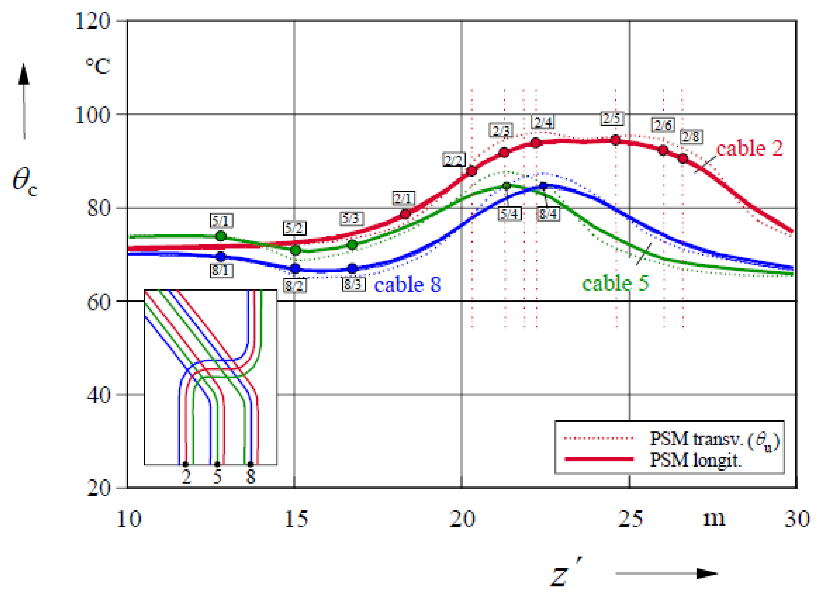
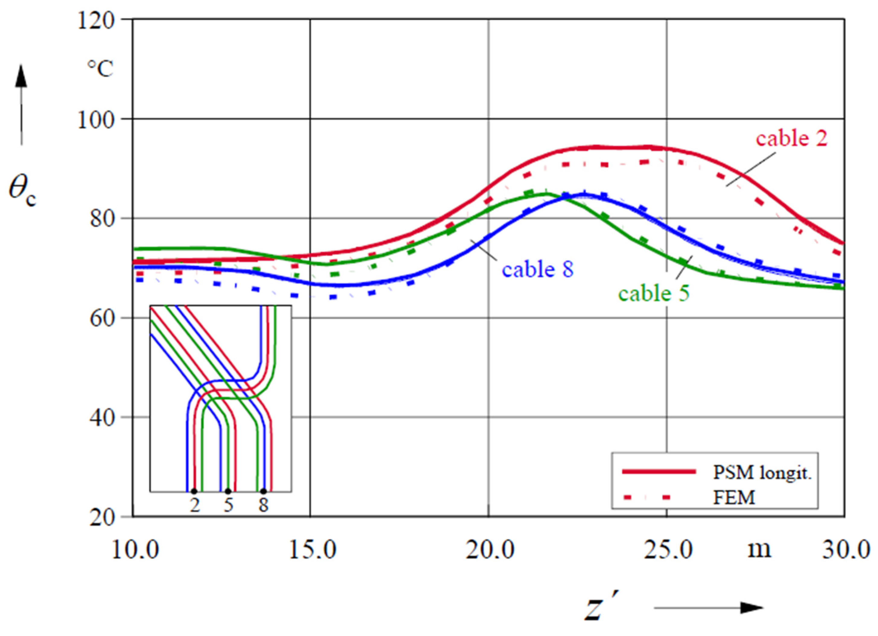
4.2. Steady State, with Consideration of the Longitudinal Heat Fluxes

Since in complex cable arrangements the conductor temperature will vary along its length because of the influence of cable crossings and changes in the surrounding environment, the longitudinal heat flow should be taken into account. This is discussed briefly below, as this subject was addressed in [16].
As before, we will assume that each cable section is (with a typical length of, e.g., 0.01 m) has constant conductor losses Wi. The temperature along the section i s was obtained in [16] as:
θ i s = A i s exp ( γ z ) + B i s exp ( γ z ) + θ u , i s
where θ u , i s denotes the uninfluenced temperature, that is, without the longitudinal heat flow, and
γ = T L T r
Let us now consider section ν with the right edge having the coordinate z′ = ν Δz. The constants A and B in (17) are obtained iteratively as [16]:
A v + 1 = A v 0.5 ( θ u , v θ u , v + 1 ) exp ( γ v Δ z ) B v + 1 = B v + 0.5 ( θ u , v θ u , v + 1 ) exp ( γ v Δ z )
The calculation starts with z′ = 0 at the left border of Subsection 1 in Section 1, that is, at a point where a negligible longitudinal heat flow can be assumed (typically at a distance of 10…20 m from the critical area). This means that:
A1 = B1
and:
B 1 = 0.5 ( θ u , 1 + v = 1 n s θ u , v { e x p [ γ ( v 1 ) z ] e x p [ γ v z ] } )
The computational algorithm starts with the assumed temperatures for all cable sections. Next, through an iterative process, new temperatures are obtained and the corresponding losses are computed. Usually, four to five iterations are required to achieve convergence with 0.1 K accuracy.
The full lines in Figure 13 show the resulting temperature distributions, compared with the foregoing distributions (thin, dotted). Comparing cable 2 with the other cables, 5 and 8, leads to the conclusion that the broad saddle of high temperatures in cable 2 is hindering longitudinal heat fluxes to the colder ends, so that the resulting temperatures are only slightly reduced.
In order to test the PSM model, finite element (FEM) studies have been performed using the same conditions as in Figure 12. The mesh generated by the COMSOL Multiphysics program is shown in Figure 14 with the comparative results shown in Figure 15.
We can observe that the results are very close, within 3 K difference. Keeping in mind that through FEM an additional longitudinal heat flow along the metal screens of the cables will be taken into account—which, e.g., in [15] caused a rating difference of nearly 1%, which again may cause a temperature difference of 1…2 K—these temperature differences are further relativized.

4.3. Transient Behaviour (without Longitudinal Heat Fluxes)

Applying (9) offers the possibility of analyzing the transient behavior of complex cable systems. The theory presented in Section 2.2 dealt with heat generated by a line source. A typical power cable is composed of several conducting and nonconducting layers, each with its own thermal capacitance. In order to account for the thermal capacitances of the internal cable components, the total temperature rise of the cable is obtained as [3]:
Δ θ c ( t ) = Δ θ i ( t ) + α ( t ) Δ θ e ( t )
where the attainment factor, defined as,
α ( t ) = Δ θ i ( t ) Δ θ i ( )
reflects the fact that the step response is initially (in a range of some hours) dominated by the inner temperature rise of the cable.
For the arrangement of Figure 12, this is done under the assumption that the cable system 1 (the cables 1…3) are steadily loaded with a current of 1600 A, whereas the other six cables are switched on with 1600 A each at the time t = 0. The losses during the considered times at t = 100 h, 1000 h, 10,000 h and 100,000 h (t ⊄ ∞) are taken from the final situation, which is shown in Figure 13 and Figure 15.

4.4. Transient Behaviour with Consideration of the Longitudinal Heat Fluxes

As an example, the installation of the nine 220-kV cables in Figure 12 is chosen and the transient case of Section 4.3. Figure 16 shows the temperature distributions for the times named above with a steady load of 1600 A in system I, whereas cables 4…9 in systems II (here: cable 5) and III (here: cable 8) are switched on at t = 0 with a load step of 1600 A. It can be seen that for t = 10,000 h the final distributions are close to the steady-state ones and for t = 100,000 h (t ⊄ ∞) are almost exactly equal to the steady-state values.

5. Conclusions

A new method for temperature and rating calculations in arbitrarily complicated cable arrangements was introduced in this paper. The PSM method results in much simpler equations than the traditional approaches. For example, for the steady-state solution, 1/r replaces the logarithm of r and in the transient case, (1/r) erfc(r, t) replaces the exponential integral EI (r, t).
The most important conclusions can be summarized as follows:
  • The most simple geometric definition is achieved by using equidistant points along the cable axis.
  • This method is much easier to handle compared with the finite line sources with their special systems of coordinates.
  • It provides a very simple formulae for expressing temperature rises, relating only to the distance r between the considered point and the point source.
  • It enables the consideration of varying temperatures along the cable conductor.
  • It enables the analysis of transient conductor temperatures even for complicated, nonlinear cable runs.
  • It enables the analysis of transient cable temperatures, taking into account the longitudinal heat fluxes, even for very complicated, nonlinear cable runs.

Author Contributions

Conceptualization: H.B.; methodology: H.B.; software: H.B., G.J.A. and P.Z.; validation: H.B. and G.J.A.; formal analysis: H.B. and G.J.A.; writing—original draft preparation, H.B. and G.J.A.; writing—review and editing, H.B. and G.J.A. All authors have read and agreed to the published version of the manuscript.

Funding

This research received no external funding.

Institutional Review Board Statement

There were no studies on human or animals in this work.

Informed Consent Statement

There is no research on humans in this work.

Data Availability Statement

There is no additional data available for this work.

Conflicts of Interest

The authors declare no conflict of interest.

References

  1. IEC 60287-1-1. Electric Cables–Calculation of the current rating-art 1-1: Current rating equations (100% load factor) and calculation of losses–General, IEC, (2014–2011).
  2. IEC 60287-2-1. Electric Cables–Calculation of the current RC. Kemp et al. Sirolex: A finite element computer program for the thermal analysis, design and monitoring of underground and aerial high and medium voltage insulated cable systems, -part 2-1: Thermal resistances (calculation of thermal resistances, IEC, (2015-1).
  3. IEC 60853-2. Calculation of cyclic and emergency rating of cables. Part 2–Cyclic rating of cables greater than 18/30 (36) kV and emergency ratings for cables of all voltages, (1989-07).
  4. Anders, G.J. Rating of Electric Power Cables–Ampacity Calculations for Transmission, Distribution and Industrial Installations; Institute of Electrical and Electronics Engineers: New York, NY, USA, 1997. [Google Scholar]
  5. Bremnes, J.J.; Evenset, G.; Stolan, R. Power. Loss and inductance of steel armoured multi-core cables: Comparison of IEC values with “2.5D” FEA results and measurements. [report B1-116, Cigre Paris Session, 2010].
  6. Sturm, S.; Paulus, J.; Berger, F.; Abken, K.-L. 3D-FEM modelling of losses in armoured submarine power cables and comparison with measurements. [report B1-215, CIGRE 2020].
  7. Pilgrim, J.; Catmuli, S.; Chippendale, R.; Levin, L.; Stratford, P.; Tyreman, R. Current Rating Optimisation for Offshore Wind Farm Export Cables. [report B1-108, CIGRE 2014].
  8. Huang, Z.; Lewin, L.; Swingler, S. Rating of HVDC Submarine Cable Crossings, report A6.2. In Proceedings of the Jicable 9th International Conference on Insulated Power Cables, Versailles, France, 21–24 June 2015. [Google Scholar]
  9. You, L.; Wang, J.; Liu, G.; Ma, H.; Zheng, M. Thermal Rating of Offshore Wind Farm Cables Installed in Ventilated J-Tubes. Energies 2018, 11, 545. [Google Scholar] [CrossRef] [Green Version]
  10. Fu, C.-Z.; Si, W.-R.; Quan, L.; Yang, J. Numerical Study of Convection and Radiation Heat Transfer in Pipe Cable. Math. Probl. Eng. 2018, 2018, 1–12. [Google Scholar] [CrossRef] [Green Version]
  11. Chippendale, R.; Cangy, P.; Pilgrim, J. Thermal Rating of J tubes using Finite Element Analysis Techniques, report B5.4. In Proceedings of the Jicable 9th International Conference on Insulated Power Cables, Versailles, France, 21–24 June 2015. [Google Scholar]
  12. Brakelmann, H. Erweitertes Verfahren zur Berechnung der Belastbarkeit kompliziert aufgebauter Kabeltrassen. In Extended Calculation Method for Current Ratings of Complicated Cable Routes; University of Duisburg-Essen: Duisburg, Germany, 1986; pp. 894–898. [Google Scholar]
  13. Anders, G.J.; Brakelmann, H. Cable crossings-derating considerations. I. Derivation of derating equations. IEEE Trans. Power Deliv. 1999, 14, 709–714. [Google Scholar] [CrossRef]
  14. Anders, G.J.; Brakelmann, H. Cable crossings-derating considerations. II. Example of derivation of derating curves. IEEE Trans. Power Deliv. 1999, 14, 715–720. [Google Scholar] [CrossRef]
  15. Anders, G.J.; Dorison, E. Derating Factor for Cable Crossings with Consideration of Longitudinal Heat Flow in Cable Screen. IEEE Trans. Power Deliv. 2004, 19, 926–932. [Google Scholar] [CrossRef]
  16. Brakelmann, H.; Anders, G.J. A new method for analyzing complex cable arrangements. IEEE Trans. Power Deliv. 2021. [Google Scholar] [CrossRef]
  17. Carslaw, H.S.; Jaeger, J.C. Conduction of Heat in Solids; Oxford Science Publications: Oxford, UK, 1946. [Google Scholar]
  18. Abramowitz, M.; Stegun, I.A.; Irene, A. Handbook of mathematical functions. In National Bureau of Standards Applied Mathematics Series-55, 10th ed.; National Bureau of Standards: Washington, DC, USA, 1972. [Google Scholar]
  19. Brakelmann, H.; Anders, G.J. Transient Thermal Response of Power Cables with Temperature Dependent Losses. IEEE Trans. Power Deliv. 2021, 2777–2784. [Google Scholar] [CrossRef]
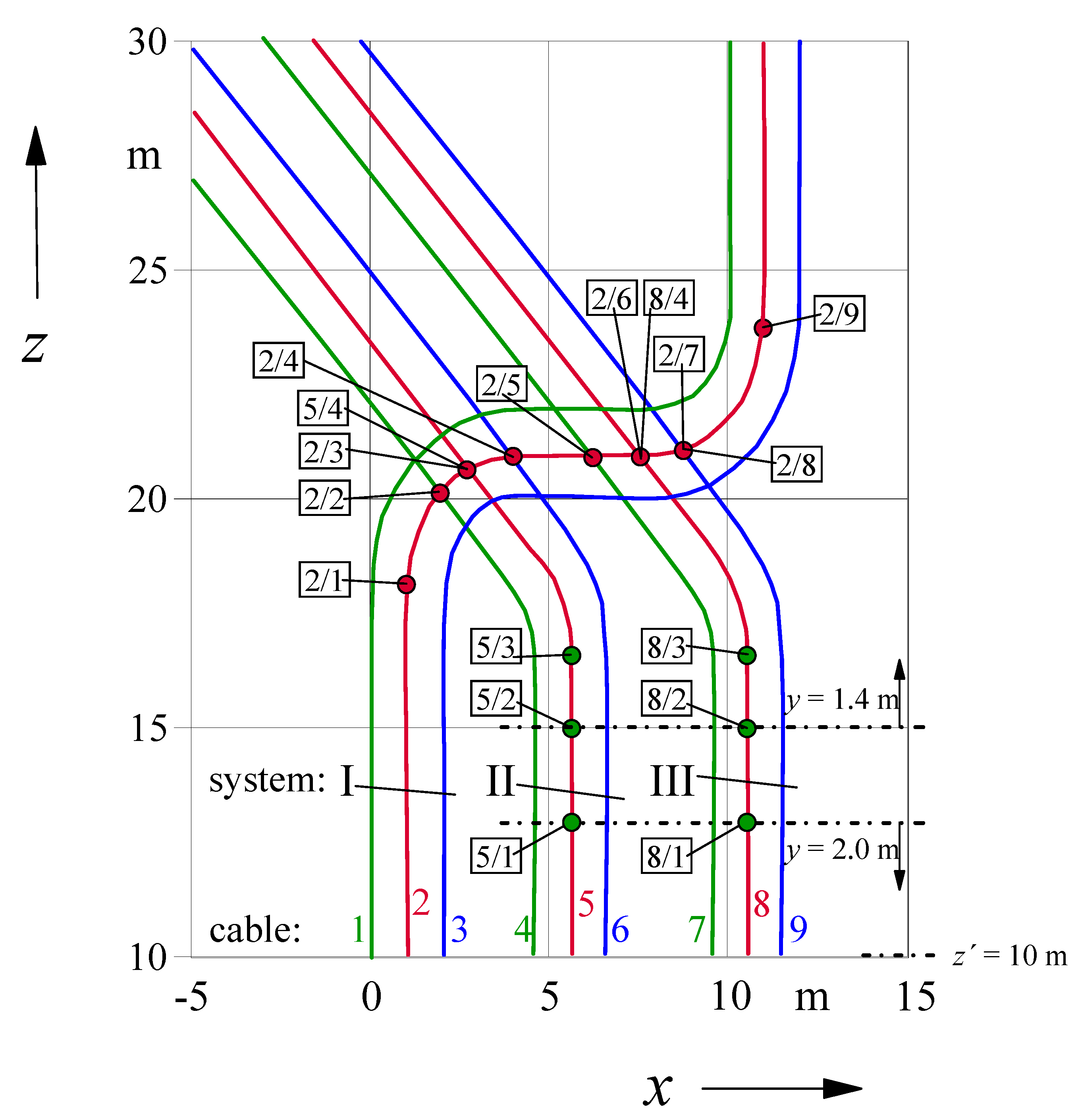
Figure 1. Point source with heat emission W, reflected at the soil surface.
Energies 14 06813 g001
Figure 2. Subdividing a line source into short sections with the length Δl and the losses W′(z′) Δl.
Energies 14 06813 g002
Figure 3. Temperature rise in the middle of a line source from z′ = −10 m to z′ = +10 m and in a distance xP from its axis (at z′ = 0), as a function of the length Δl. The line source is represented by point sources of length Δl and losses (p.u.l.) of W′ = 100 W/m; depth: y = 2.0 m (dotted: infinite line source). The first diagram (a) shows the location of point xp with respect to the line source with the parameter the distance of this point from the center line [Figures a) to d)].
Energies 14 06813 g003aEnergies 14 06813 g003b
Figure 4. Temperature rise caused by a semi-infinite line source (as the “missing continuation”).
Energies 14 06813 g004
Figure 5. Temperature deviation in a considered point from Figure 3 at a distance of Δz from the end of the finite line source; parameter: distance xP from the z-axis; depth: y = 2.0 m (dotted lines correspond to an infinite line source).
Energies 14 06813 g005
Figure 6. Thermal step responses (9) of a line (z′= −30 … + 30 m) with point sources (green lines Δl = 0.01 m), each with a loss step of WΔlW= 100 W/m) at t = 0, at a distance Δy below the line (y = 2.0 m, at z′ = 0 m), compared with the step responses (10) of infinite line sources (red lines, mostly hidden).
Energies 14 06813 g006
Figure 7. Finite line of point sources with locally varying losses (L = 2.0 m; Δl = 0.01 m; λ = 1.0 W/(K m)).
Energies 14 06813 g007
Figure 8. Thermal response at a point with Δy = 0.05 m to a finite line of point sources with loss steps of 100 W/m and 150 W/m, as defined in Figure 7.
Energies 14 06813 g008
Figure 9. Line source with a 90° bend with the bending radius R and a depth of y = 2.0 m.
Energies 14 06813 g009
Figure 10. Temperature rise of a point 0.05 m below the line source (y = 2.05 m) with a bending radius R; losses (p.u.l.) W′ = 100 W/m.
Energies 14 06813 g010
Figure 11. Transient temperature rise in the considered points of Figure 9 with maximum temperature rise for a loss step (p.u.l.) of W′ = 100 W/m at t = 0; parameter: bending radius R.
Energies 14 06813 g011
Figure 12. Crossing area with complex arrangement of nine 220-kV-XLPE-cables (3 × 3 × 1 × 2500 mm2 copper; 60 Hz) with a laying depth of y = 2.0 m for z < 13.0 m; cables 4…9 are rising between z = 13.0 …15.0 m from y = 2.0 m to y = 1.4 m; distance of axes in all systems: 1.0 m; current in all cables: 1600 A (15 °C; 1.0 W/(K m)).
Energies 14 06813 g012
Figure 13. Distributions of the conductor temperatures of the middle cables 2, 5 and 8 in Figure 12 along the particular cable axes (z′); for explanations of the special points, see Figure 12 and Table 1. Abbreviations: transv. refers to the radial heat transfer only, whereas longit represents both radial and longitudinal heat flows.
Energies 14 06813 g013
Figure 14. Mesh for the cable arrangement in Figure 12.
Energies 14 06813 g014
Figure 15. Comparison of the MPS and FEM results for middle cables of each circuit in Figure 12.
Energies 14 06813 g015
Figure 16. Conductor temperatures of the middle cables 2, 5 and 8 Figure 12: in system I (cable 2) with a steady load of 1600 A, whereas in systems II (cable 5) and III (cable 8) with load steps of 1600 A at t = 0 in cables 4…9; temperature distributions for (a) t = 100 h, (b) 1000 h, (c) 10,000 h, (d) 100,000 h; for explanations of the special points: see Figure 12 and Table 1.
Energies 14 06813 g016
Table 1. Explanations of the special points in Figure 12.
PointxyzzExplanation
mmmm
cable 2
2/11.002.0018.0018.00beginning of bend 1
2/21.802.0020.2020.40crossing point with cable 4
2/32.702.0020.7021.35crossing point with cable 5
2/43.702.0021.0022.50crossing point with cable 6
2/56.022.0021.0024.72crossing point with cable 7
2/67.412.0021.0026.14crossing point with cable 8
2/78.022.0021.0026.70beginning of bend 2
2/88.702.0021.1026.72crossing point with cable 9
2/911.002.0024.0031.40end of bend 2
cable 5
5/15.592.0013.0013.00beginning of cable rising (L = 2.0 m)
5/25.591.4015.0015.00end of cable rising (L = 1.4 m)
5/35.591.4016.5916.70beginning of the bend
5/42.701.4020.7021.90crossing point with cable 2
cable 8
8/110.592.0013.0013.00beginning of cable rising (L = 2.0 m)
8/210.591.4015.0015.00end of cable rising (L = 1.4 m)
8/310.591.4016.5916.70beginning of the bend
8/47.411.4021.0022.30crossing point with cable 2
Publisher’s Note: MDPI stays neutral with regard to jurisdictional claims in published maps and institutional affiliations.

