A Review of Multi-Objective Optimization in Organic Rankine Cycle (ORC) System Design

Abstract

Organic Rankine cycle (ORC) is considered a promising heat-to-power technology to utilize waste heat and renewable energy, including solar, biomass and geothermal. However, since the thermodynamic, economic and environmental performance is usually conflict, the single objective design could no longer meet the requirements of the ORC system, putting forward urgent requirements for multi-objective optimization, which has attracted increasing attention with lots of papers published. However, due to these different decision variables, optimization objectives and approaches, existing research is significantly different from each other and is difficult to compare without a systematic summary. Therefore, this paper provides an overview of ORC multi-objective research from three perspectives: optimization objective, method and optimization parameters. Based on the classification of different objectives, this work summarizes the involved variables and provides a recommendation for selecting appropriate objectives in different scenarios. For the optimization method, this work compares different approaches and reveals their advantages and disadvantages. Finally, the decision variables are reviewed and classified into four levels. Then the integrated design approach considering “system-process-component-fluid” is proposed and recommended for further development.

1. Introduction

Energy and climate crises are the common challenges facing mankind. Reducing fossil fuel consumption, increasing the proportion of renewable energy and energy efficiency are beneficial to realizing carbon neutrality in the middle of this century, which has become the consensus of the world. Organic Rankine cycle is a widely used power system in utilizing medium-to-low temperature thermal energy, which could effectively use renewable energy, including solar energy, geothermal energy, biomass energy and ocean energy [1]. Furthermore, ORC could also recover waste heat resources, including industrial waste heat and engine waste heat [2]. Therefore, ORC could improve the proportion of renewable energy, increase energy efficiency and reduce carbon emissions, thereby showing huge application potential in a low-carbon energy system in the future [3].

In the past decade, ORC has attracted widespread interest from worldwide scholars with an amount of research conducted. These studies mainly focus on system optimization design, working fluid selection, cycle configuration improvement, component design and control strategies, which have made significant progress [4]. Particularly, as the basis of fluid selection, component design and configuration comparison, system optimization has attracted the most attention [5]. Early research only aims to optimize a single objective, usually the maximum thermal efficiency or net output power. As the research develops, the economic and environmental performance of ORC systems such as the total cost, payback period (PBP), levelized cost of energy (LCOE), net present value (NPV), total carbon emission and sustainability indicator (SI) have gradually attracted increasing attention. Results show that different optimization objectives are often contradictory and cannot be optimal simultaneously [6]. Therefore, the multi-objective optimization of ORC systems was proposed and developed. Up to date, the multi-objective optimization method has become increasingly popular in ORC system design.

The multi-objective optimization (MOO) means that the number of optimized objectives is more than two, as shown in Equation (1). The N is the number of target variables, and M is the number of optimized variables, namely the decision variable. Here, g(x) is the inequality constraint, and h(x) is the equality constraint. Essentially different from the single-objective optimization, MOO will not result in a single solution, but a series of trade-off solutions, which is called the Pareto frontier, meaning that no objective could be improved without sacrificing any other objectives [7,8]. From the mathematic perspective, all trade-off solutions are equally important in theory. However, a single solution should be selected to guide the practical engineering according to the preference information, which is usually characterized as the weight.

$$\begin{array}{l}\min y=f(x)=\left[f_1(x),f_2(x),f_3(x)\dots ,f_n(x)\right], n=1,2,3,\dots ,N\\ g(x)\le 0, i=1,2,3,\dots ,I\\ h(x)=0, j=1,2,3,\dots ,J\\ x=\left[x_1,x_2,x_3,\dots ,x_m\right], m=1,2,3,\dots ,M\end{array}$$

(1)

Recently, there have been many researches discussing the MOO in ORC system design. For instance, Wang et al. focused on maximizing the thermal efficiency and minimizing the heat exchanger area per power output of the subcritical ORC using the simulated annealing algorithm [9]. Yang et al. optimized the evaporator/condenser pressure and superheat degree to minimize the total investment cost and maximize the W_net, using the multi-objective Genetic algorithm [10]. Furthermore, the MOO method has also been used in working fluid selection [11]. Feng et al. carried out a thermo-economic comparison between pure and mixture fluids in ORC, in which the exergy efficiency and Levelized energy cost (LEC) are selected as the objective variables [12,13]. Xi et al. proposed a graphical criterion, namely the Pareto frontier, to distinguish the optimal fluid for waste heat recovery, in which the exergy efficiency and annual cash flow were considered [14]. Ghasemian et al. compared eight fluids from the perspective of thermal, exergy and cost. Results indicated that dry fluids have a better performance of costs and exergy efficiency than wet fluids [15]. Moreover, the MOO method could be used to compare different ORC architectures. Lecompte et al. explored the specific investment cost (SIC) and total power output (W_net) of subcritical and transcritical ORC using the Non-dominated Sorting Genetic Algorithm II (NSGA-II). Results indicated that subcritical ORC shows lower W_net but with better economics [6,16]. Sadeghi et al. compared the simple ORC, parallel two-stage ORC and series two-stage ORC from the viewpoints of turbine size and W_net. Results indicated that STORC outperforms other configurations under the same conditions [17]. Song et al. compared the subcritical, transcritical, superheated and recuperated ORC considering the exergy efficiency and payback period Results indicated that the superheating is more suitable for the fluids with lower critical parameters, while the recuperation is not attractive under most operating conditions [18].

In general, MOO has been widely applied in ORC, from system design to cycle configuration and to fluid selection. The involved objectives are also numerous, including the conventional thermodynamic indicators such as exergy efficiency, power output and also the economic indicators such as the LCOE and SIC. Moreover, there are also multiple optimization methods such as the NSGA-II and weighted sum method (WSM). Due to these different decision variables, optimization objectives and approaches, existing researches are significantly different with each other and are difficult to compare or evaluate. Therefore, this work is carried out with two main purposes. The first is to review the optimization objectives, methods and variables involved in the existing research and summarize the main findings. The second is to refine further the important issues that deserve additional attention to provide valuable references for future work.

Authors searched on the Web of Science using the keywords of “multi-objective” and “organic Rankine cycle (Including other expressions: multi objective, multi criteria, bi-objective, tri-objective, Pareto, ORC.)”. Then, based on the searched results, the literature is further judged whether its focus is on ORC, removing the combined systems such as CCHP or CHP. Finally, a total of 122 papers are obtained and analyzed in this work, which are directly related to multi-objective optimization of ORC system design. As Figure 1 shows, most papers are published after 2015, revealing the popular trend of MOO in system design. There are mainly six chapters in this work. The second section discusses the optimization objectives from thermodynamic, economic, environmental and safe indicators. The third section summarizes the popular optimization methods and further compares their advantages/disadvantages. The fourth section classifies main decision variables from the system, process, component and fluid level. This work has two main contributions: (1) Summarize the main progress made in the existing multi-objective research and provide specific suggestions for selecting optimization objectives and methods in ORC optimization. (2) Propose a four-level design approach considering “system-process-component-fluid” aspects, which could design ORC architecture, component structure and working fluid molecules simultaneously. This approach is expected to improve the overall performance further and is worthy of future discussion.

2. Optimization Objective

Optimization objective is also called the target variable in MOO, referring to the variables to be maximized or minimized. The earliest and most studied evaluation indicator is the thermodynamic criterion, including the power output, thermal efficiency and exergy efficiency. Gradually, the economics attract increasing attention, including the total costs, area power ratio (APR), electricity production cost (EPC) and the specific investment cost (SIC) [19,20]. As the climate crisis deepens, the environmental performance has also been quantified and evaluated in ORC, including carbon emission and sustainability indicators. Moreover, due to the diversification of ORC application scenarios, some special needs should be considered. For instance, ORCs deployed on mobile devices to recover exhaust heat should simultaneously consider the space limitations, equipment weight and safety. In this section, different indicators in ORC will be sorted out and analyzed.

According to the optimization objective, all 122 papers are counted and classified. A list of all reviewed papers could be found in the Supplementary Material, and this section mainly summarizes the key findings. Figure 2a shows the paper number involving different indicators. Results indicate that the thermodynamic criterion is the most popular indicator, especially the exergy efficiency, accounting for almost half of all papers. The economic criterion is followed, including the LCOE, SIC and total cost. In contrast, there are very few studies on environmental performance, volume, weight and safety. Only nine papers calculate the total carbon emission with four papers discussing the sustainability index. Figure 2b shows the number of objective indicators. The majority of studies (75%) only focus on bi-objective optimization. 16% of studies focus on tri-objective optimization. In contrast, only one study discusses the optimization with over five objectives, due partly to the immaturity of high-dimensional optimization methods, which will be discussed in Section 3.

2.1. Thermodynamic

As the most basic index in ORC, the thermodynamic criterion indicates the system’s ability to utilize heat sources, which is usually quantified by the power output, thermal efficiency and exergy efficiency. The basic concepts and equations are listed in Appendix A and will not be discussed in the main part.

Usually, the designer only chooses one of the power output and thermal efficiency as the optimization objective, according to the specific application scenario. In terms of thermal efficiency, it is more popular in solar or biomass ORC since the thermal oil cycle is usually included. This oil cycle belongs to the closed system defined by Zhai et al. [21], which is more suitable for efficiency evaluation. In contrast, the power output is more suitable for an open system, including the industrial waste heat, engine waste heat, geothermal and other scenarios without oil cycle, as shown in Figure 3. In these open systems, the outlet heat is directly discharged without being recycled.

The traditional exergy loss analysis for each component helps facilitate the optimal design of the component and ORC system [22]. Furthermore, the advanced exergy analysis methods have become increasingly popular in recent years, which decomposes the exergy loss into endogenous and exogenous parts, thereby determining the possibility of reducing the loss through technological improvement [23]. Therefore, if the endogenous loss of all components is summed up, the efficiency improvement limit of the ORC system could be obtained. For instance, Wang et al. used advanced exergy analysis to estimate the improvement potential of dual-loop ORC. Results indicated that the high-temperature turbine is the first component that needs technical modifications [23].

2.2. Economic

In addition to the thermodynamic performance, the economic criterion is also an important indicator to evaluate ORC performance, which has become a necessary option for ORC optimization. Up to date, the popular indicators include the indirect indicator, and direct indicators (total cost, SIC, PBP, etc). Particularly, exergoeconomic analysis is different from traditional economic analysis and deserves additional discussion.

2.2.1. Indirect Indicator

Indirect indicators do not directly measure the cost or economics of the whole ORC sysem, but use the parameters such as heat exchanger area to characterize the component cost qualitatively [24]. The commonly used index includes heat exchanger internal heat transfer requirement (UA) [25,26], heat exchanger area, turbine size, area to power ratio (APR) [27] and other indexes.

Specifically, the UA is simple to use since only the heat capacity and temperature difference are needed without complicated iterative calculation for U. Feng et al. used UA as an economic evaluation index to evaluate the cost of a supercritical-subcritical ORC in waste heat utilization [28]. Tiwari et al. optimized the exergy efficiency and the total UA of the evaporator and condenser. For a known working fluid, the total UA will exhibit the required area [29]. Further, the heat transfer coefficient U could be calculated to determine the heat exchanger area based on various heat exchange correlations [30]. Gotelip et al. designed the heat exchanger to minimize the total heat exchanger area and maximize the power of ORC in floating product storage offload [31]. The turbine diameter is also selected as the optimization objective to obtain a smaller turbine size [32]. Bahadormanesh et al. defined an objective function by dividing the turbine inlet radius by power output [33]. Rahbara et al. minimized the overall turbine size (d_max) for a highly compact ORC layout applied in diesel truck engines [34]. However, the smaller area or diameter does not necessarily represent lower costs since the impacts of material, pressure level, component structure are not considered [35].

These indirect indicators could only characterize the cost of a certain component. However, they could not represent the overall economy of the overall ORC system. For different system sizes, the results are difficult to compare, either. Therefore, more direct indicators are required to represent the costs of the whole ORC system.

2.2.2. Direct Indicator

Direct indicators are much more frequently used in existing research since they are strictly defined in engineering or economics, including the Total cost, Specific investment cost (SIC), Payback period (PBP), Levelized cost of electricity (LCOE), Net present value (NPV) and Internal Rate of Return (IRR), as shown in

Table 1. Comparison of different economic indicators.

Indicator	Definition	Advantage	Disadvantage
Ctot	Total investment cost	Easy to use;	Not consider time value or technical criterion
SIC	Specific investment cost	Easy to use; simultaneously consider cost and power;	Not consider the time value
PBP	Payback period	Consider time value	Not consider system lifetime
LCOE	Levelized cost of energy	Compared with electricity price to determine the feasibility	Need to presume multiple parameters; significantly affect the results.
NPV	Net present value	Intuitively shows the profitability	Difficult to presume return rate
IRR	Internal rate of return	Not affected by external parameters; dependent on the cash flow	Calculation is complex

. Total cost is the most basic index to evaluate ORC economics [36], which are mainly calculated using empirical correlations, fitted from the equipment cost on the market [37]. The two most popular correlations are from Turton [38] and Smith [39]. In Sun’s work, the carbon emission costs and water consumption costs were also considered [40]. Based on total cost, SIC describes the unit cost per power output [41] and has the advantage of easy use and intuitive comparison between different cases. Sun et al. maximized the exergy efficiency and minimized the specific power cost, revealing the better performance of double pressure ORC over traditional ORC [42]. However, SIC does not consider the depreciation, operation costs or discount rate [43]. PBP measures the number of years required to recover the total cost, including the static and dynamic ones. Generally, the dynamic PBP is more usual since it considers the time value over multiple years. For instance, Wang et al. used dynamic PBP to evaluate the superiority of the ORC investment plan in engine waste heat recovery [44]. LCOE denotes the cost of unit electricity and could be directly compared with the local electricity price to represent the profitability. In addition, the comparison between different energy generating technologies is also convenient, as suggested by Lecompte [6]. It’s worth noting that many existing researches also use other abbreviations such as EPC or LEC to represent the cost per power generation, especially in the research of industrial/engine waste heat [45,46,47]. In this review, these abbreviations are unified as LCOE.

The net present value (NPV) intuitively shows the profitability during the lifetime operation. Hu et al. used NPV to evaluate the total profits of a hybrid geothermal-solar power system during the 30-year operation [48]. Pirerobon et al. used NPV to evaluate the profitability of three waste heat recovery units for offshore platforms [49]. However, the expected discount rate should be defined in advance, which is related to the company’s lowest investment rate of return and is usually difficult to determine. In contrast, IRR has an outstanding advantage in that it depends entirely on investment cash flow and is not affected by external parameters, including the discount rate [50]. However, IRR only represents a ratio rather than an absolute value. When the project scale is large, a low IRR may also result in large profits. Therefore, it is suggested that IRR and NPV should be simultaneously considered when comparing different schemes. In general, authors recommend the direct indicators in ORC design, especially the LCOE, NPV and IRR, which describe the lifetime economy of the entire system, rather than individual component or static periods.

2.2.3. Exergoeconomic Analysis

Exergoeconomic analysis combines advanced exergy analysis and economic analysis, aiming to explore the relative importance of each component in the design of the ORC system [51]. Different from the normal economic analysis, exergoeconomic analysis also calculates the exergy cost rate when considering the equipment cost and operation cost [52,53]. Özahi et al. calculated the capital cost rate of components using the SPECO method to determine the optimal fluid from toluene, MDM, D4 and n-decane [54]. Behzadi et al. identified the relative cost importance of each component and designed a cost-effective ORC system for waste recovery. Results indicated that R123 is the best working fluid from exergy efficiency and total production cost [55].

2.3. Environmental

The research on environmental performance started later than thermodynamic and economic performance. The most studied environmental performance is the carbon emission. Moreover, there are also some studies on sustainability indicators (SI) [56].

2.3.1. Carbon Emission

Carbon emission is the most intuitive and commonly used environmental indicator. The emissions of ORC system involve all processes through the whole life cycle, including production, transportation, operation and recycling. Specifically, the emission sources include: (1) the process of manufacturing the components, (2) leakage of organic fluids in operating process, (3) replacement of coal/natural gas using ORC. Some researches also discuss the impact of recycling water on carbon emission [57]. Moreover, the methane also results in the greenhouse effect, which could be converted into carbon emissions using coefficients. Common analysis method includes the Total equivalent warming impact (TEWI) method, Life cycle climate performance (LCCP), life cycle analysis (LCA) and carbon emission coefficient method, which are described in detail:

(1)

Total equivalent warming impact (TEWI)

TEWI method is a measure of the greenhouse gas emissions, with the advantages of simple calculation and easy application. TEWI is mainly composed of two parts [58]: (1) direct emission: emissions caused by fluid leakage and end-of-life recovery. (2) Indirect emission: energy saving due to ORC power. Yang et al. introduced an extended TEWI method to evaluate the impact of refrigerants on climate change, considering that the generated power of ORC could compensate for the warming relief [58].

(2)

Life cycle climate performance (LCCP)

LCCP is developed based on the TEWI method, which considers chemical manufacturing and end-of-life disposal compared with TEWI, as shown in Zhang’s work [36]. The diagram of LCCP is shown in Figure 4.

(3)

Carbon coefficient

The carbon coefficient method is a general method for direct multiplication coefficient to calculate carbon emissions. For instance, power generation could multiply a coefficient to estimate carbon emissions [23]. Xia et al. calculated the warming value considering the conversion factor of CO₂, CO and CH₄ based on coal-fired power plants [59].

(4)

Life cycle analysis (LCA)

LCA is a standardized method based on ISO 14,044 [60], which could evaluate the environmental effects in each stage during the life cycle, including the construction, operation, maintenance and disposal [61]. Herrera et al. assessed the exergo-environmental performance of the waste heat recovery systems with simple and regenerative ORC. Results indicated that toluene presented the best efficiency and lower climate effects with 0.00181 kg CO₂ eq·kWh⁻¹ [62].

Table 2. Typical references involving carbon dioxide emission.

Reference	Method	CO2 Source
		CH4 Equivalence	Component Construction	Working FLUID Leakage	Power Reduction	Other
Wang et al. [23]	Carbon coefficient	√	√		√
Herrera et al. [62]	LCA		√	√	√
Xia et al. [59]	Carbon coefficient	√	√		√
Zhang et al. [36]	LCCP		√	√	√
Yi et al. [63]	LCA	√	√	√
Martinez et al. [57]	TEWI		√	√	√	Water consumption
Kalikatzarakis et al. [64]	Carbon coefficient	√			√

summarizes related researches on carbon emission. Results show that existing studies usually calculate emission from two or three categories. However, no research has considered all factors simultaneously, which may underestimate the ORC’s environmental performance.

2.3.2. Exergoenvironmenal Analysis

Exergoenvironmenal analysis has a similar principle to advanced exergy analysis by linking the environmental impact with the energy flow and internal inefficiency, which is different from the direct calculation of carbon emission [53]. Fergani et al. compared three fluids in cement industry ORC by taking the exergy efficiency, cost and environmental impact per exergy unit of the net produced power as optimization objectives. Results indicated that benzene is the best from an exergo-environmental point of view [65].

2.3.3. Sustainability Index (SI)

The definition of SI is the ratio of exergy loss rate to the exergy decline of heat source (water, exhaust gas), which is used to evaluate the impact of ORC on the environment [66]. The key idea is to improve the exergy efficiency, reduce the emitted heat and alleviate the damage to the environment [67]. A lower SI means a smaller impact [68].

2.4. Other

In addition to the thermodynamic, economic and environmental indicators, there are also other evaluation indicators, including system volume, weight and safety.

2.4.1. Volume

ORC could be used on mobile vehicles and marine scenarios. Due to the limited space, ORC volume is a very important factor in these scenarios. Many researchers focus on the volume of the heat exchanger since it is the largest component in the ORC system. For instance, Xu et al. [69], Baldasso et al. [70], Liu et al. [71], Barbazza et al. [72] optimized the system parameters and structure by taking the heat exchanger volume as the optimization objective. Moreover, some researchers also consider the volume of turbines, feed pumps and auxiliary equipment [73]. Based on each component’s structure, related empirical correlations could also be used to calculate the volume [74].

2.4.2. Weight

Similar to the volume, the weight of the ORC system is also an important factor in mobile vehicles. Imran et al. [73] and Pierobon et al. [49] used correlation equations to calculate the weights of turbines, heat exchangers, feed pumps, pipes, instrumentation/control systems and other auxiliary components. Then an additional mass of 10% is supplemented to represent the mass of storage tanks. Finally, the total weight is selected as one of the optimization objectives. More detailed equations could refer to these references.

2.4.3. Safety

Safety is a very important index in all application scenarios but is seldom discussed. Safety mainly refers to the risk of workers when exposed to the ORC environment, which is usually measured by the individual risk [57]. These risks are mainly caused by the leakage of flammable and toxic working fluids and high-pressure pipes. There are special methods for quantitative safety assessment, such as the Quantitative Risk Analysis (QRA).

Lee et al. simplified the QRA method and focused on the riskiest part, namely the pipeline between the feed pump and evaporation, since the pressure is the highest in this process [75]. The authors focused on source modeling, dispersion modeling and fire event modeling, and used the concept of risk distance to characterize the ORC safety. In addition, some scholars directly optimize the ORC system from the perspective of fluid design to minimize the flammability, thereby improving ORC safety. Papadopoulos et al. researched the molecular design of mixed fluids by minimizing the flammability of two pure fluids using the group-contribution method [76].

2.4.4. Stability

Most of the aforementioned studies only discuss a single working condition. During the practical operation, the ORC system always deviates from the design condition due to the influence of solar radiation, wind speed and ambient temperature. Therefore, some scholars take the power fluctuation as the optimization objective, and minimize the fluctuation range as small as possible by parameter optimization.

Li et al. focused on solar-based ORC and selected the fluctuation of output (W·min⁻¹) as the optimization objective [77]. Results indicated that a larger energy storage capacity could reduce power fluctuation, but will significantly increase the costs. Bufi et al. focused on maximizing the thermal efficiency and minimizing its variance [78]. Zhang et al. proposed a multi-objective estimation of distribution algorithm to keep superheat following a target value by controlling the pump speed [79].

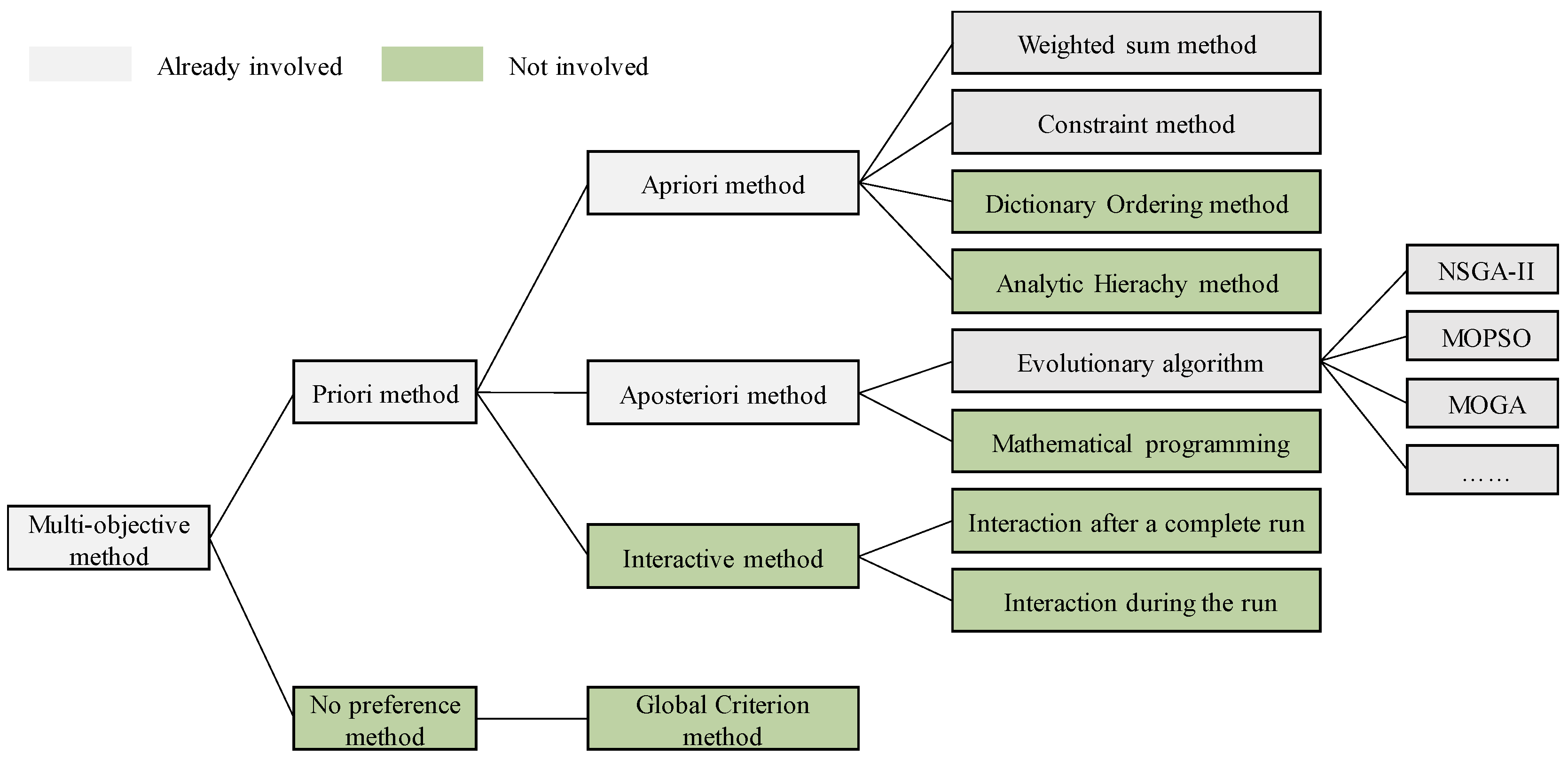
3. Optimization Method

Multi-objective optimization method is essentially different from single-objective optimization. A single optimal solution could be obtained in single-objective optimization. However, different indicators compete with each other, and there is no unique optimal solution in multi-objective optimization (MOO), which is also more complex and time-consuming to converge. MOO is usually divided into the Priori method and No preference method. Further, the Priori method could be divided into the Apriori method, interactive method and Aposteriori method, according to whether the preference information is determined before, during or after the optimization process, as shown in Figure 5. At present, the Apriori method and evolutionary algorithm method are widely used in ORC, including the linear weighted sum method (WSM), ε-constraint method and smart algorithms such as NSGA-II, MOPSO and etc.

This work has summarized the application of these methods in the ORC MOO application, as shown in Figure 6 [7,80]. Results show that, from the perspective of optimization methods, many interesting methods have not been applied in ORC, including the interactive methods that could feedback the decision makers’ preferences during the design process. Applying these methods may make the system design more in line with the needs of designers and engineering projects, thus worth future exploration.

In particular, MOGA and NSGA-II are both developed from the single-objective Genetic algorithm and are not distinguished in many previous researches. Therefore, this review uses NSGA-II to represent these two methods. Results show that NSGA-II is the most popular algorithm, accounting for about 66% of all existing studies. The second popular method is WSM, which accounts for 16%. Other methods such as MOPSO and ε-constraint method only account for 18%. Therefore, this work will take WSM, ε-constraint and intelligent algorithm as examples to introduce the principle and application in detail, and compare the advantages and disadvantages of each method.

3.1. Weighted Sum Method (WSM)

3.1.1. Principle

WSM combines multiple target variables into a single one according to a certain weight ratio, thereby transforming the multi-objective optimization problem into a simpler single-objective optimization problem [81], as shown in Equation (2).

$$f(x)={\omega }_1{f}_1(x)+{\omega }_2{f}_2(x)+\dots +{\omega }_N{f}_N(x)$$

(2)

where w represents the weight factor, ranging from 0 to 1. The sum of all factors is 1.

WSM has a simple principle and is easy to use. There is no theoretical upper limit to the number of optimization objectives. Thus 2, 3, 5 or even more than 10 objectives could be combined into one [82]. For instance, Arasteh et al. combined the thermal efficiency and exergy efficiency into one objective function with each factor’s contribution of 0.5. Then the Genetic Algorithm is used to solve this optimization problem [83]. Zhu et al. combined the exergy efficiency and the heat exchanger area per power output into one function. Then the optimization is conducted to determine the optimal evaporation temperature, condensation temperature and working fluid [84]. In addition to the Genetic algorithm, the PSO could also be used to solve this single-objective problem [71].

3.1.2. Methods to Determine the Weight

WSM is a priori method with the weight and preference being determined before optimization. Thus a consequent problem is: how to determine the weight factor of each target variable? In many previous studies, the weight factor is directly assumed. For instance, the weight is usually set as 0.5:0.5 [83,85] or 0.6:0.4 [56] when two target variables are used. When four target variables are considered, the weight is usually set as 0.1:0.2:0.3:0.4 [86]. This direct assumption usually only considers typical weight scenarios but is too subjective and does not consider the characteristics of each target variable. Therefore, in some researches, the weight factor is not subjectively determined by the designer, but using other mathematical models to calculate the coefficient according to each variable’s characteristics. The typical methods include: the α-method, Analytic Hierarchy Process (AHP), and Grey relational analysis (GRA) [87].

(1).

α-method

α-method calculates the weight factor by considering the magnitude and the range of each optimization objective. A variable with a larger range will have a larger weight to ensure that two indicators have similar magnitudes after multiplying the weight [68,88]. This method is usually used for bi-objective optimization, in which the weight factor could be calculated by:

$${\omega }_1=\frac{f_2^{\max }-f_2^{\min }}{(f_1^{\max }-f_1^{\min })+(f_2^{\max }-f_2^{\min })}, {\omega }_2=\frac{f_1^{\max }-f_1^{\min }}{(f_1^{\max }-f_1^{\min })+(f_2^{\max }-f_2^{\min })}$$

(3)

α-method is simple and easy to use. However, the maximum and minimum value of two optimization objectives should be determined in advance, which could be calculated through four single-objective optimizations, thereby significantly increasing the calculation complexity. For instance, Kazemi et al. firstly determines the weight coefficients of exergy efficiency and SIC using the α-method, and then explores the effects of system parameters [89].

(2).

Analytic Hierarchy Process method (AHP)

The AHP method is a kind of multi-criteria decision-making method, which divides complex problems into orderly levels to make them organized. Then the importance of each element is quantitatively compared and described, which could be used to calculate the weight factor of each variable, as shown in Figure 7 [90].

Zhang et al. discussed four target variables, including power, thermal efficiency, exergy efficiency and carbon emission by dividing these variables into four levels: energetic, exergetic, economic and environmental criteria. Then the author used nine absolute numbers (1–9) to indicate the importance intensity (equal, moderate, strong, extreme importance and etc.) and construct the judgment matrix [36]. It is worth noting that different indicators should be dimensionless.

(3).

Taguchi method

Taguchi method is a statistical method to obtain the importance of different factors to the objective function, which could be used in the experiment, theory and numerical simulation [91]. Bademlioglu used this method to explore the impact of changes in different ORC parameters on system thermal efficiency and exergy efficiency. The author first used this method to obtain an orthogonal array of optimization objectives (thermal and exergy efficiency). Then this array is converted into a signal-to-noise (S/N) ratio in 27 cases. Consequently, the weight factors could be calculated as 52.61% and 47.38% [91].

3.2. ε-Constraint

The core idea of the ε-constraint method is to regard a single indicator as the optimization objective and convert other objectives into constraints, thereby transforming the multi-objective optimization problem into a single-objective optimization problem. Different from the WSM method, ε-constraint could deal with the non-convex problems [63].

$$\begin{array}{l}\min f_i(x)\\ f_j(x)\in {\epsilon }_j(j=1,2,\dots ,M,j\ne i)\end{array}$$

(4)

Multiple calculations could result in a relatively complete Pareto frontier. However, Figure 8 shows that if the ε is too small, f₁ may exceed the feasible region, resulting in non-convergence. If ε is too large, there will be more feasible solutions, resulting in lower convergence speed. Therefore, some prior knowledge is often needed to determine a reasonable range of ε. For instance, Yi et al. firstly conducted two single-objective optimizations to determine the lower and upper bounds. Then authors implemented the ε-constrained method to solve this multi-objective optimization problem in GAMS 23.6 [63].

3.3. Intelligent Algorithm

Regardless of the WSM or the ε-constraint method, there is either the invalidity of the non-convex problem or the requirement for prior information, resulting in limitations to practical application. As the algorithm develops, some intelligent optimization algorithms with wider applicability have been gradually developed and improved, which have been widely used in different fields.

Popular intelligent algorithms include the NSGA-II [33], MOPSO [92], MOEA [93]. Non-dominated Sorting Genetic Algorithm II (NSGA-II) is an improved algorithm for NSGA based on GA’s selection, crossover and mutation ideas, which was proposed by Deb in 2001 [94] It is worth mentioning that the gamultiobj function embedded in the Matlab toolbox is also a modified version of NSGA-II. Therefore, this review uses NSGA-II to simultaneously characterize the method of self-programming or calling the Matlab toolbox. The multi-objective particle swarm optimization (MOPSO) algorithm was proposed by Carlos A. Coello in 2004 for multi-objective optimization based on the PSO algorithm [95], which simplifies the crossover and mutation process and shortens the convergence time. The disadvantage of PSO is that it is easy to fall into local optimization, resulting in low convergence accuracy and poor solution diversity. Multiobjective Evolutionary Algorithm Based on Decomposition (MOEA/D) transforms the multi-objective optimization into a single-objective problem with the advantage of lower computational complexity [96]. The disadvantage is that the weight vectors need to be set artificially, which will determine the quality of the final solution [96].

In addition to the intelligent algorithms mentioned above, there are also other algorithms applied in ORC, including the multi-objective heat transfer search (MOHTS) [97], Artificial Cooperative Search (ACS) [98], multi-objective grey wolf optimizer (MOGWO) [99], multi-objective firefly algorithm (MOFA) [33], artificial bee colony algorithm (ABC) [100] and simulated annealing (SA) [101]. Even though these methods are rarely used, it will still be a very interesting topic to compare these different methods. However, for high-dimensional optimization with 4 or more objectives, these intelligent algorithms are currently ineffective since the calculation time will increase significantly and the solution is not accurate, either. Therefore, WSM method is recommended for three or more optimization objectives, as shown in

Table 3. Comparison of different multi-objective optimization methods.

Optimization Method	Advantages	Disadvantages	Recommended Scenario	Case
Weighted sum method	·Simple, easy to use ·could include multiple objectives (>10)	·Pareto is not uniform ·cannot tackle the nonconvex problem ·need normalization for objectives	Ns ≥ 4	[20]
ε-constraint	·could tackle the nonconvex problem	·calculation time varies for different formulations ·Pareto is not uniform ·epsilon is difficult to determine	-	[63]
Intelligent algorithm	·could tackle the nonconvex problem ·Pareto is uniform	·only include several objectives (<4) ·time consuming ·multiple adjustable parameters	Ns ≤ 3	[44,102]

.

3.4. Decision Making

The multi-criteria decision-making method (MCDM) develops from scheme sorting in operations research and is also used to select the optimal solution from the Pareto in the MOO of ORC. This decision-making process selects the optimal solution for design guidance according to the decision maker’s preference [103]. In ORC optimization, the typical MCDM methods include TOPSIS, LINMAP, Shannon entropy, GRA, fuzzy set theory, etc. The differences between these methods lie in the definition of the optimal solution. For instance, LINMAP only requires the solution closest to the ideal one [104], while TOPSIS requires the solution closest to the ideal solution and the farthest from the non-ideal one at the same time [105,106]. The Shannon entropy method could measure the uncertainty with information sources using the probability theory [107]. The key point is that the objective with a sharp distribution will have lower importance compared with that following the biased distribution [13]. As a part of grey system theory, grey relational analysis defines the black area, white area and grey area [108]. Theoretically, this analysis proposes a dependence to measure the correlation degree of factors, meaning that more similarity leads to more factor correlation [40].

Statistical results in Figure 9 show that nearly half of the multi-objective optimization studies use the MCDM method to determine the optimal solution. TOPSIS is the most popular approach, accounting for over 60%. LINMAP comes next, accounting for about 35%, while Shannon entropy and GRA methods are relatively less used. Since these MCDM methods have various concepts and usually lead to different final solutions, some researchers propose to apply multiple methods simultaneously and then determine the final solution using the aggregation method, which may improve the robustness of the decision-making process [13,90,103]. Detailed descriptions are shown in

Table 4. Descriptions of different MCDM methods.

Refs.	Method	Principle	Calculation
[109,110,111]	LINMAP	Closest to the ideal solution	$d_{i+}=S_i^{*}=\sqrt{{\displaystyle \sum _{j=1}^N{(V_{ij}-V_j^{*})}^2}}$
[112,113,114]	TOPSIS	Closest to the ideal solution. Furthest to the non-ideal solution.	$d_{i-}=S_i^{-}=\sqrt{{\displaystyle \sum _{j=1}^N{(V_{ij}-V_j^{-})}^2}}$$C_i^{*}=\frac{d_{i-}}{d_{i-}+d_{i+}}$
[13,107]	Shannon entropy	A sharp distribution leads to lower importance	$S{E}_j=-\frac{1}{\ln (n)}{\displaystyle \sum _{i=1}^n{P}_{ij}\ln P_{ij}}$
[40,44,59,108,115]	Grey relational analysis	More similarity leads to more factor correlation	${\xi }_i(k)=\frac{\min ({\Delta }_i(\min ))+\rho \max ({\Delta }_i(\max ))}{\left|x_0(k)-x_i(k)\right|+\rho \max ({\Delta }_i(\max ))}$

.

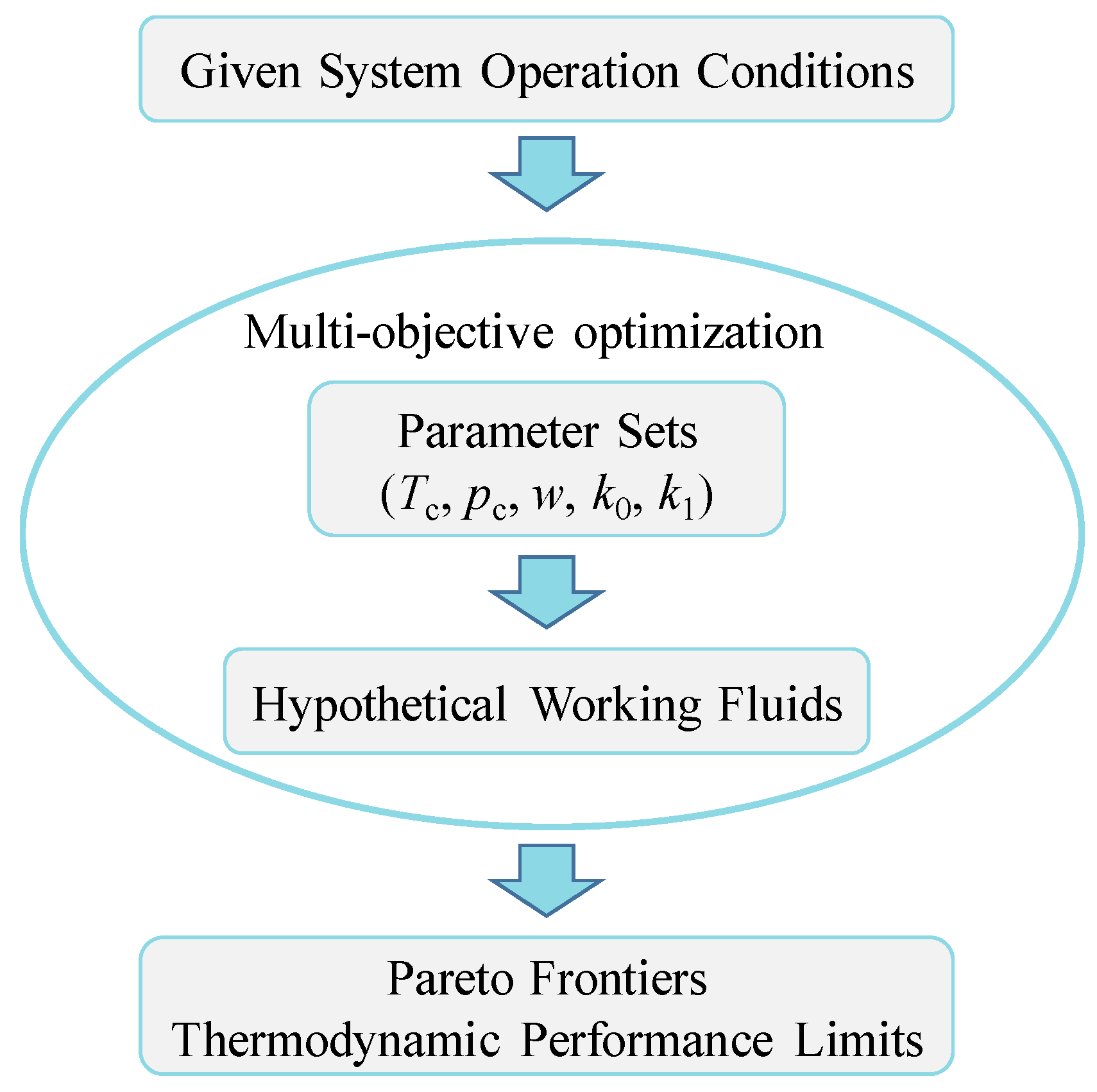
4. Optimization Parameter

During the MOO process, many ORC parameters could be optimized. The most popular ones are evaporation pressure, superheat, condensation pressure and other parameters, which all belong to the system level. In addition, there are also some parameters at the component level and working fluid level that could be optimized, which will be discussed in detail in this section.

4.1. System Level

System-level optimization parameters mainly include the evaporating pressure/temperature, condensing pressure/temperature, subcooling and superheating. Under given conditions of heat source, the efficiency and net power output of ORC could be calculated according to the above system-level parameters. For the transcritical ORC, the superheat degree is not required, but the evaporation pressure and turbine inlet temperature should be determined at the same time [6,52]. For other new architectures such as dual-pressure evaporation ORC and two-stage ORC, the optimized parameters are more but are similar to the simple cycle [116]. System-level parameters are the most basic parameters of ORC, which are involved in almost all ORC optimization researches and will not be discussed in detail.

4.2. Process Level

Process-level design mainly refers to the design of cycle processes and system configurations, such as the conventional subcritical cycles, transcritical cycles, two-stage cycles, multi-pressure evaporation cycles. Most of the existing researches select the configuration by directly comparing the Pareto frontier of different forms through multi-objective optimization. However, this comparison could only study simple and several configurations. When there are multiple possible configurations, the computational complexity will increase sharply. Superstructure optimization could discuss various alternative configurations by analyzing the process stream, thereby parameterizing the ORC process design. Then the intelligent algorithms could be used to quickly solve the problem and obtain the best system structure and process, as shown in Figure 10. Kermani et al. [117] conducted a superstructure modeling for ORC systems driven by industrial waste heat, including regenerative, superheating, turbine-bleeding, reheating, multi-stage and transcritical cycles, etc. The multi-objective optimization is carried out with the net power output and total cost as the objective. Results indicate that the coupling of multiple forms results in better economics and thermodynamic performance.

4.3. Component Level

In addition to the system-level and process-level parameters, the parameters at the component level also have a very significant impact on ORC performance. Key ORC components include the turbine, evaporator, condenser and feed pump. Up to date, most existing studies focus on the heat exchanger or the expansion device. The heat exchangers mainly include the shell-and-tube heat exchanger, plate heat exchanger and tube-fin heat exchanger. The expansion device mainly includes the radial turbine, axial turbine and scroll expander [118]. It is worth mentioning that no multi-objective optimization on the feed pump is discovered in this literature review. Part of the reason may be that the cost of the feed pump is much lower than that of the turbine or heat exchanger. However, as one of the key components in ORC, the efficiency of the feed pump has a significant impact on system efficiency and operational stability. Therefore, the structural design of the feed pump could be further discussed in the future.

(1).

Heat exchanger

The heat exchanger is an important and also the largest component in ORC, including the evaporator, condenser, regenerator, preheater and superheater. The structure design of the heat exchanger is beneficial to reducing the exergy loss, improving system efficiency and increasing the safety and stability of ORC operation. Generally, the heat exchanger includes shell-and-tube, plate, tube-fin and plate-fin type [106,119,120]. The structure and optimization parameters of different heat exchanger types are also different, as shown in

Table 5. Comparison of different heat exchangers.

Type	Advantages	Disadvantages	Application Scenario
Shell-and-tube	Mature, lower cost, long life	Large volume, low heat transfer coefficient	For liquid-liquid heat exchange
Plate	High heat transfer coefficient, low heat loss, compact structure, small volume	Poor sealing, only low pressure, higher flow resistance	For liquid-liquid and liquid-gas exchange
Tube-finned	High heat transfer coefficient, compact structure	Complex structure, expensive	For liquid-liquid and liquid-gas exchange
Plate-finned	High heat transfer coefficient, compact structure	Easy to block, poor resistance to corrosion	For liquid-liquid, liquid-gas and gas-gas exchange

.

In terms of the shell-and-tube heat exchanger, the optimization parameters mainly include the tube diameter, shell diameter, baffles spacing, tube number and tube length. In terms of the plate exchanger, the popular decision variables include the plate number, plate length, plate thickness, plate spacing, channel length, channel width and pass number. More detailed parameters are shown in Table 6.

(2).

Expansion device

The expansion device is the key component in ORC, which could be divided into the turbine, scroll expander and screw expander according to the power range. Ref. [118] introduces the categories and applications of different expansion devices in ORC. This work aims to reveal the parameters and turbine types in multi-objective optimization. According to the literature, most existing researches focus on radial turbine but pay little attention to other turbine types. The popular decision variables include the expansion ratio, specific speed, blade angle, blade height, radius ratio and flow coefficient. For an axial turbine, only Schilling et al. [121] have optimized the turbine stages but not discuss other structural parameters such as inlet angle and turbine size. For the positive displacement shown in Figure 11, both scroll expander and screw expander are more suitable for medium and small-scale ORC systems. However, there is currently no published work on incorporating expander structure parameters into the multi-objective optimization of ORC, which is worthy of further research.

Table 6. List of the reference focusing on the component level.

Component	Type	Year	Author	Optimized Parameter
Heat exchanger	Shell-and-tube	2021	Turgut et al. [22,98]	Outer tube diameter, shell diameter, baffles spacing, number of tube passes, tube arrangement.
	double-pipe tubular	2019	Van Kleef et al. [122]	Working fluid velocities
	Tube-finned, plate-finned	2019	Holik et al. [123]	Length, width, height.
	Tube-finned	2019	Baldasso et al. [70]	Inner tube diameter, tube length, fin height, fin thickness, fin spacing, transversal pitch
	Shell-and-tube	2019	Baldasso et al. [70]	Inner tube diameter, tube length, baffle spacing
	Tube-finned	2017	Liu et al. [71]	Inlet radius on tube, Inlet radius on shell, fin eight, fin thickness, fin spacing.
	Shell-and-tube	2016	Andtreasen et al. [11]	Inner tube diameter, number of tubes, Baffle spacing
	Plate	2015	Lecompte et al. [6]	Number of passes
	Plate	2015	Kalikatzarakis et al. [64]	Number of plates, plate thickness, plate length, channel length, channel width
	Plate	2015	Imran et al. [124]	Channel length, channel width, plate spacing
	Shell-and-tube	2014	Pierbon et al. [49]	Inner tube diameter, tube length, number of tubes, baffle spacing
	plate-finned	2014	Pierbon et al. [49]	Fin height, fin frequency, fin length, number of plates, flow length
	Plate	2014	Barbazza et al. [72]	Plate width, channel spacing, number of channels, number of passes
	Plate	2013	Wang et al. [125]	Plate length, plate width, channel distance
	Shell-and-tube	2013	Pierbon et al. [74]	Outer diameter, tube pitch, baffle spacing
Turbine	radial	2021	Li et al. [126]	Expansion ratio, specific speed
	radial	2021	Alshammari et al. [127]	Rotor blade angle, exit vane angle, blade thickness, vane thickness
	radial	2020	Jankowski et al. [128]	Specific speed
	radial	2019	Palagi et al. [129]	Specific speed, specific diameter
	radial	2019	Bekiloglu et al. [32]	Specific speed, radius ratio
	axial	2017	Schilling et al. [121]	Turbine stages
	radial	2017	Bahadormanesh et al. [33]	Velocity ratio, rotational speed, inlet flow angle, radius ratio, meridional velocity ratio
	radial	2017	Al Jubori et al. [130]	Flow coefficient, nozzle radius ratio, rotor radius ratio, Rotational speed
	radial	2015	Rahbara et al. [34]	Expansion ratio, rotational speed, flow coefficient, radius ratio
	radial	2015	Erbas et al. [131]	Flow coefficient, inlet blade height, inlet flow angle, exit flow angle, number of blades, meridional speed ratio

Table 6. List of the reference focusing on the component level.

Component	Type	Year	Author	Optimized Parameter
Heat exchanger	Shell-and-tube	2021	Turgut et al. [22,98]	Outer tube diameter, shell diameter, baffles spacing, number of tube passes, tube arrangement.
	double-pipe tubular	2019	Van Kleef et al. [122]	Working fluid velocities
	Tube-finned, plate-finned	2019	Holik et al. [123]	Length, width, height.
	Tube-finned	2019	Baldasso et al. [70]	Inner tube diameter, tube length, fin height, fin thickness, fin spacing, transversal pitch
	Shell-and-tube	2019	Baldasso et al. [70]	Inner tube diameter, tube length, baffle spacing
	Tube-finned	2017	Liu et al. [71]	Inlet radius on tube, Inlet radius on shell, fin eight, fin thickness, fin spacing.
	Shell-and-tube	2016	Andtreasen et al. [11]	Inner tube diameter, number of tubes, Baffle spacing
	Plate	2015	Lecompte et al. [6]	Number of passes
	Plate	2015	Kalikatzarakis et al. [64]	Number of plates, plate thickness, plate length, channel length, channel width
	Plate	2015	Imran et al. [124]	Channel length, channel width, plate spacing
	Shell-and-tube	2014	Pierbon et al. [49]	Inner tube diameter, tube length, number of tubes, baffle spacing
	plate-finned	2014	Pierbon et al. [49]	Fin height, fin frequency, fin length, number of plates, flow length
	Plate	2014	Barbazza et al. [72]	Plate width, channel spacing, number of channels, number of passes
	Plate	2013	Wang et al. [125]	Plate length, plate width, channel distance
	Shell-and-tube	2013	Pierbon et al. [74]	Outer diameter, tube pitch, baffle spacing
Turbine	radial	2021	Li et al. [126]	Expansion ratio, specific speed
	radial	2021	Alshammari et al. [127]	Rotor blade angle, exit vane angle, blade thickness, vane thickness
	radial	2020	Jankowski et al. [128]	Specific speed
	radial	2019	Palagi et al. [129]	Specific speed, specific diameter
	radial	2019	Bekiloglu et al. [32]	Specific speed, radius ratio
	axial	2017	Schilling et al. [121]	Turbine stages
	radial	2017	Bahadormanesh et al. [33]	Velocity ratio, rotational speed, inlet flow angle, radius ratio, meridional velocity ratio
	radial	2017	Al Jubori et al. [130]	Flow coefficient, nozzle radius ratio, rotor radius ratio, Rotational speed
	radial	2015	Rahbara et al. [34]	Expansion ratio, rotational speed, flow coefficient, radius ratio
	radial	2015	Erbas et al. [131]	Flow coefficient, inlet blade height, inlet flow angle, exit flow angle, number of blades, meridional speed ratio

4.4. Fluid Level

Different organic working fluids significantly affect ORC performance. Therefore, determining a suitable working fluid from diverse types of fluids is particularly important for the practical application of ORC. In general, the current research on the selection of working fluids is divided into two levels. The first level is to compare the ORC performance when using different working fluids directly. The second level is to design the working fluid, that is, the working fluid is parameterized using the equation of state or the molecular group. Therefore, the second level is not limited to existing organic fluids, but can also calculate the ORC performance using potential working fluids in the future. This section will introduce the research status of these two fluid levels.

4.4.1. Selection from Limited Fluids

Most researches are based on comparing existing working fluids, including the pure fluids or mixtures. The typical approach is to construct the ORC model and calculate system performance, in which the physical property is obtained from software such as REFPROP or CoolProp. This method has the advantages of simplicity and high accuracy since most of the physical parameters in REFPROP have been verified and fitted by experiments.

(1)

Pure fluids

The optimization of pure fluid is mainly reflected in the comparison of ORC performance using different fluids but does not discuss or design the fluid itself. Therefore, the pure fluid will not be expanded in detail in this work. For more discussion, please refer to the existing literature [132].

(2)

Mixture

Due to the temperature slide during the phase change process, zeotropic mixtures could obtain a better temperature matching with heat/cold source, thereby reducing the heat loss in the heat exchanger and improving system performance. Different composition ratios could result in different temperature slides. Thus the design of zeotropic mixture mainly focuses on optimizing the component ratio, especially the ratio of binary mixtures [133]. However, the application potential of ternary or quaternary mixture is less discussed and could be explored in the near future.

4.4.2. Fluid Design

Even though the comparison of existing fluids is easy to conduct, it is usually difficult to determine the optimal fluid from diverse working fluids since the calculation process needs to be repeated many times, which significantly increases calculation time. Moreover, the direct selection of working fluids can only be based on existing working fluids. These diverse fluids usually have different critical temperatures, critical pressures, flammability and toxicity, which are difficult to quantify and compare with each other. Therefore, some researchers propose to incorporate the fluid characteristics into the design optimization of the ORC system, which is usually called computer-aided molecular design (CAMD) [122]. Currently, there are two popular molecular design methods. One is the contribution group design method, which calculates the physical properties of fluid by determining its chemical structure through the contribution group design. The other approach is to use the general equation of state (EOS) to parameterize the working fluid by characterizing the physical properties of the working fluid with critical temperature, critical pressure and eccentricity factor [134]. Consequently, the fluid characteristics could be included in the optimization process. In this section, the two methods will be introduced.

(1)

Group-contribution method (GCM)

The principle of GCM is that through the combination of different structural groups (—CH₃, =CH-), any kind of organic fluid can be constructed theoretically. As shown in Figure 12, popular organic fluids in ORC such as R601a and R134a can be represented using the combination of common structural groups [135]. Using this principle, the physical properties of the working fluid are determined by the number of each group and its contribution ratio. In this GCM method, the contribution of each group is considered the same, regardless of the specific spatial structure and location. Therefore, the GCM method can predict the physical properties of both existing working fluids and also unknown fluids. GCM has a much faster calculation speed than CCM but has less accuracy.

Papadopoulos et al. used the GCM method to generate a series of ORC candidate fluids, including existing fluids and also novel fluids. Then the optimal fluid is selected considering the requirements of safety and environmental performance [76,136,137]. Van Kleef et al. used the GCM method to estimate the critical physical properties and transport properties of the working fluid. Then the authors used a multi-objective optimization method to optimize the thermodynamic and economic performance simultaneously, and explored the optimal working fluid design in different heat source conditions [122]. Moreover, Su et al. reviewed the application of the GCM method in ORC and summarized the commonly used equations for predicting different macroscopic parameters of working fluids, such as boiling point, critical physical properties, transport properties, flammability and toxicity [135].

(2)

Equation-of-State method (EOS)

The equation of state method uses a few parameters, including the critical parameters and eccentricity factors, to calculate the basic and transport properties of a certain working fluid. In this way, the fluid properties and the thermodynamic and economic performance of the ORC system could be calculated. In traditional physical property software such as REFPROP, although high-precision multi-parameter equations of state can be used to accurately obtain the thermophysical properties of the working fluid, these equations have many adjustable parameters and require a large number of experimental fittings. The forecast for novel fluids is not precise enough for ORC performance prediction. In contrast, the general-purpose state function is simpler and has fewer parameters, which can be more reliably extended to unknown working fluids, as shown in Figure 13 [134,138].

Yang et al. proposed a corresponding states model to predict the fluid properties using five parameters: critical temperature, critical pressure, acentric factor, molar ideal gas isobaric heat capacity and temperature gradient [134]. In this way, different working fluids could be parameterized. The authors compared 13 common existing fluids and obtained the thermodynamic performance limit, which characterizes the best performance that can be obtained by improving the working fluid under ideal conditions.

(3)

Computational chemistry method (CCM) method

In addition, there is a computational chemistry method (CCM) from the view of autom, which has a too long convergence time (usually from hours to days for a molecular structure). Therefore, this CCM method is not currently suitable for fluid design in the ORC system [135]. Comparison of three CAMD methods is shown in

Table 7. Comparison of three computer-aided method for property prediction.

Method	Advantages	Disadvantages	Appropriate for Cycle Optimization?	References
CCM	Accurate	Time consuming, (hours to days for one molecule)	×	[135,139]
GCM	Wide range, efficient for new fluids	Less accurate	√	[76,122,136]
EOS	Quite accurate	May be inefficient for new fluids	√	[134]

.

5. Discussion and Future Outlook

The single-objective optimization could no longer meet the requirements from the increasingly serious climate crisis, different technical requirements and rich application scenarios. Instead, the thermodynamic, economic, environmental and other performance should be considered simultaneously, which, however, usually conflict with each other. Thus it is difficult to obtain a unique optimal solution, proposing challenges to ORC multi-objective optimization. In recent years, there have been increasing studies involved in multi-objective optimization and discussing the ORC design. Correspondingly, multi-objective optimization has also become increasingly popular and gradually become a typical method for system design.

5.1. Discussion

In general, existing research has made significant progress, which could promote the development of many new indicators or methods and lay the basis for the practical application of the ORC system. The progress could be divided into the following areas:

5.1.1. Optimization Objective

The optimization objectives of the ORC system have been greatly enriched, including the thermodynamic, economic, environmental indicators, as well as the system weight, volume, safety and stability, which provide valuable guidance for the design and operation of ORC system. Different indicators have their advantages, disadvantages and application scopes, which are also summarized in this article. However, most of the existing research focuses on thermodynamic performance, followed by economic performance, and less attention to other properties. Especially when the climate issue becomes increasingly important, the research on the environmental protection performance of the system, the role of emission reduction, and the positioning of the ORC system in low-carbon energy scenarios are still insufficient.

In terms of selecting the optimization objective, unless specific preferences are required, authors are recommended to consider the thermodynamic, economic and environmental performance simultaneously. Other indicators such as safety could be represented by the working fluids. For each category, a single indicator could be selected according to the practical application scenario, as shown in

Table 8. Recommended optimization objectives for different ORC applications.

Application	Electric Market	Electricity Benchmark Price
Geothermal, industrial waste heat	W + LCOE + Carbon emission	W + IRR + Carbon emission
Solar, biomass (with oil cycle)	ηth + LCOE + Carbon emission	ηth + IRR + Carbon emission
Engine waste	W + LCOE + Carbon emission + Volume + Weight

. The power output and thermal efficiency are recommended for thermodynamic performance. Particularly, the power output is more suitable for geothermal, waste heat scenarios, which does not include the thermal oil cycle. In contrast, the thermal efficiency is more suitable for solar, biomass scenarios with oil cycles. In terms of the economic criterion, LCOE and IRR are recommended since these two indexes are independent of system size. The calculation of IRR is based on electricity price, thereby being more suitable for the region with a benchmark price. In contrast, LCOE describes the electricity price and is more suitable for the region with the electricity market. Particularly, LCOE is applicable for engine waste heat recovery in cars or marine applications since the electricity is usually consumed locally and not sold to the grid. Moreover, the system volume and weight should also be considered in these waste heat scenarios since the volume is very limited.

Specifically, for calculating the carbon emission, the combination of LCA and the carbon coefficient method is recommended. This combined method could calculate the carbon emission during production and transportation, and also consider the emission reduction by replacing other plants using ORC, thereby improving the accuracy over separate LCA or carbon coefficient method.

5.1.2. Optimization Method

As the algorithm develops, ORC optimization approaches are also gradually improved. The number of optimization objectives increases from a single one to two, three and multiple. The approach varies from the linear weighting method to the ε-constraint method, and the intelligent algorithms, which could obtain the Pareto frontier more conveniently. Furthermore, based on the Pareto frontier, many studies introduce the multi-criteria decision theory to select the desired solution with corresponding weights. Thus the unique solution could be determined to guide engineering design according to the decision maker’s preference. However, most of the studies are based on optimization with three or fewer objectives. When the objective number exceeds three, the current intelligent algorithms could not converge very well. Up to date, only the traditional weighted method could be used to deal with high-dimensional optimization (>3) by combining multiple indicators into one. However, this method only considers a special scenario, and the weight is difficult to determine.

Based on this review, the authors recommend the intelligent algorithms in the optimization with 2-3 objectives, such as the NSGA-II, which is relatively simple to use and could effectively solve non-convex problems. These non-convex problems are very common in the design of configuration and system planning in complex thermal systems [140], which cannot be effectively solved by the WSM method. However, when the optimization objectives are more than or equal to 4, these intelligent algorithms such as NSGA-II could not work effectively with an explosive computation time and poor convergence at this stage. Therefore, the authors recommend the WSM method for this high-dimensional optimization. The specific weights can be calculated according to the AHP or α-method discussed in Section 3.1.

In addition, when using intelligent algorithms for optimization, it is usually necessary to adopt a decision-making method to obtain a unique solution for engineering applications. The authors recommend using multiple decision-making methods simultaneously by comparing the decision-making results to determine the final solution, which could effectively improve the robustness of decision-making.

5.1.3. Optimization Parameter

According to Chapter 4, the optimization parameters involved in existing research cover four levels: working fluid, components, processes and systems. Particularly, the system level is the most studied, focusing on the optimization design of evaporation/condensing pressure, superheat degree and etc. The research on process mainly aims to design the system structure and architecture by establishing a superstructure model. The research on components focuses on heat exchangers (tube and shell type, plate type and etc.) and turbines (mainly radial), while little attention is paid to feed pumps. For the working fluid, the general approach of using the group contribution method or the equation of state method to determine the optimal working fluid has been widely applied. However, the current research only focuses on one of these levels, and the research on multi-objective optimization of ORC systems considering multiple (four) levels is still scarce.

Authors recommend the collaborative design approach by considering multiple levels, especially the system, fluid and component levels. At the fluid level, the GCM or the EOS method could be used to parameterize the physical properties of the fluid and incorporate them into decision variables. At the component level, component size and structural parameters could also be included in the optimization parameters. Finally, a comprehensive design method considering four levels of system-process-component-fluid will be developed.

5.2. Future Outlook

In view of the above research status and problems, the following directions need to be developed.

5.2.1. Discussion on Carbon Emissions

The climate issue has become a major challenge threatening human survival. To achieve carbon neutrality, it is necessary to make concessions or even sacrifice certain economics. Therefore, future attention to environmental performance needs to be further strengthened.

Even though ORC could use turn heat resources into treasure (power), it is not completely carbon-free. Existing studies have used various methods such as LCA, LCCP, TEWI to measure its carbon emissions during the manufacturing process. However, there are some important issues that need further exploration, including: (1) Under the existing energy structure, how much room for emission reduction could be achieved by large-scale promotion of ORC? (2) In the future energy structure with a high proportion of renewable energy, how does ORC’s emission reduction compare to its lifetime carbon emissions? Should ORC be promoted on a large scale? (3) With the continuous improvement of the carbon trading market, could ORC independently or in conjunction with other units benefit from the carbon trading market?

5.2.2. High-Dimension Optimization

When the number of optimization objectives exceeds 3, the results and convergence of existing intelligent algorithms, including NSGA-II and MOPSO, cannot meet the requirements. At present, only a few studies have focused on high-dimensional multi-objective optimization [36,64,86,141], and the methods used are mainly linear weighted method or multi-criteria decision-making method. However, as mentioned above, the weights should be determined in advance, which makes their application limited. Therefore, the following issues need to be further discussed: (1) How to simultaneously consider multiple indicators such as thermodynamic, economic, environmental and safety index for high-dimension Pareto optimization? (2) How to reasonably convert the preferences of decision-makers and the constraints of practical projects such as limited funds and limited equipment space into weights and reflect them in the objective function?

5.2.3. Consider the Practical Operation

Most of the existing multi-objective optimizations are based on design conditions. That is, the heat source and environmental conditions are assumed the same. However, this assumption is inconsistent with practical operating conditions, resulting in significant differences between expected operation and practical operation [111], or even leading to completely opposite conclusions [142,143]. Therefore, some research proposed to integrate long-term off-design operation into the system design process. Specifically, the typical heat source conditions and ambient temperature are selected as boundary conditions to guide the multi-objective design, resulting in a more robust design scheme [116,144]. Even though this method is closer to practical engineering, it also has limitations such as time-consuming calculations and uncertain weather and heat source conditions. Even though Hu et al. proposed an approach to reduce the calculation time using the ANN method, a duration of 1–2 days is still required [48]. Yang et al. and Feng et al. proposed a BPNN model based on experimental data [145,146], but the mapping between environmental fluctuation and ORC output needs to be further established. To improve the practicability of this off-design approach, some novel methods need to be improved to reduce the calculation time and improve precision. The following aspects could be explored in the future: (1) How to integrate the dynamic response of ORC into system design? Especially the unit response speed (for heat exchanger or heat storage) and the loss during the start-stop process. (2) How much impact does the fluctuation of user-side load have on ORC design? (3) How much influence will participation in the carbon trading market have on system design? (4) How to improve the design method to speed up the optimization process based on a large number of off-design conditions and dynamic responses? Possible methods may include deep learning methods such as CNN, and the specific approach still needs to be developed.

5.2.4. Multi-Level Optimization

At present, most researches focus on the optimization of the system level, or the coupling of the two levels such as “system-component” and “system-fluid”. There is still a lack of collaborative design of “system-process-component-fluid”, which may further improve the results over conventional system optimization or component design, as shown in Figure 14. In this integrated design process, there are numerous decision variables, including the physical parameters of the working fluid, the structural parameters of components, the process parameters and the system parameters. Therefore, the optimization method and calculation capabilities need certain requirements. In general, the following aspects need further exploration: (1) Existing studies paid little attention to fluid pumps. How does the structural design of the fluid pump affect the thermodynamic and economic performance of the ORC system? (2) How much could the proposed “system-process-component-fluid” method improve system performance compared with conventional methods? What is the computational cost? (3) What’s the difference between optimization results of four levels, three levels and two levels? Which level of optimization is most appropriate considering the improvements and computation cost?

6. Conclusions

A single evaluation indicator could no longer meet the development needs of power systems such as ORC. Collaborative optimization considering multiple indicators such as thermodynamic, economic and environmental indexes has become an inevitable trend in system design. This article summarizes the research on multi-objective optimization of ORC system design. From the perspective of optimization objective, optimization methods and optimization parameters, this work classifies and statistically summarizes the existing research, and prospects the future development. Main conclusions are as follows

• For the optimization objectives, multiple aspects should be considered, including the thermodynamic, economic and environmental indicators, which should be selected according to specific application scenarios and the local electricity market. For the thermodynamic indicator, the output power is recommended for geothermal and waste heat. Thermal efficiency is recommended for solar energy and biomass. For economics, LCOE is recommended for benchmark electricity price, and IRR is recommended for the electricity market. Furthermore, for the waste heat recovery in mobile transportation, additional attention should be paid to the ORC volume and weight.
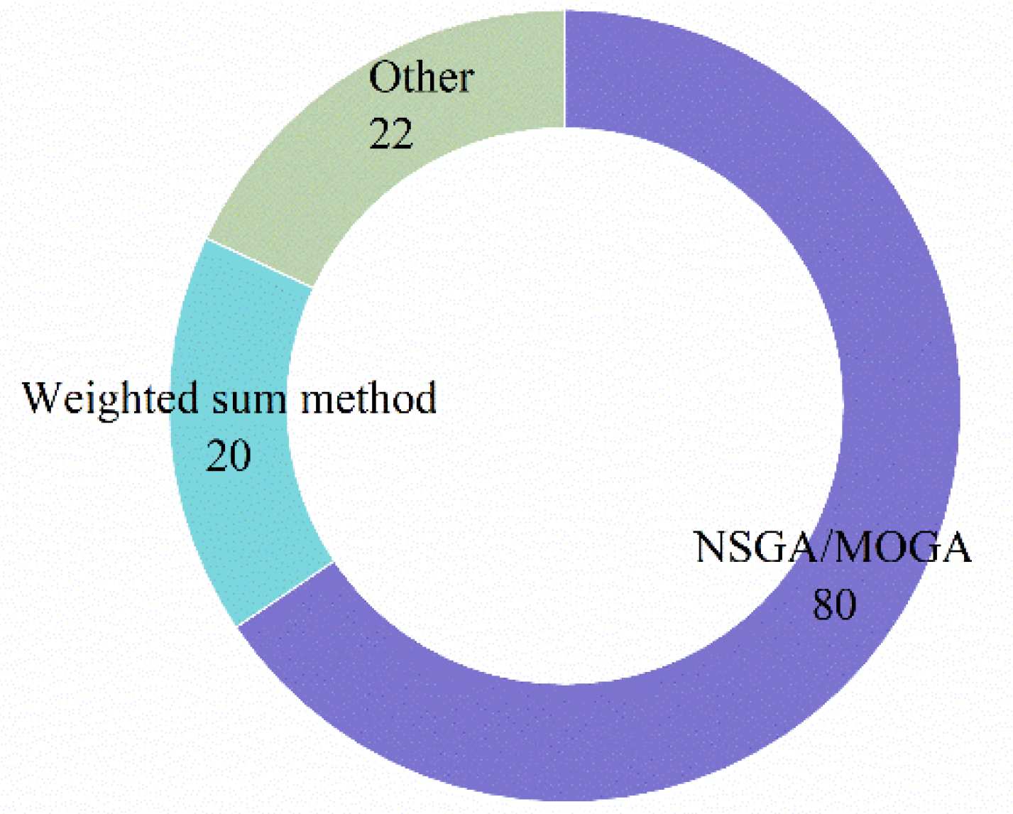
• In terms of the optimization method, intelligent algorithms including NSGA-II and MOPSO are recommended for low-dimension optimization (objective is less than 4). In contrast, the WSM method is recommended for high-dimension optimization (the objective number is more than 3), which should determine the weight in advance and then convert the complex problem into single-objective optimization.
• For optimization parameter, the researches are mainly carried out from four levels: system, process, component and fluid. However, the existing researches are relatively independent. A comprehensive design method that couples multiple levels simultaneously is expected to improve the system performance further.
• For future development, the following aspects could be further explored: (1) Exploring the emission reduction potential of ORC in the future high-proportion renewable energy system and its economic value in the carbon trading market. (2) Transform the preferences and engineering constraints into boundary constraints in multi-objective optimization. (3) Propose and expand the comprehensive optimization methods considering four levels “system-process-component- fluid”.

References

1. Roumpedakis, T.C.; Loumpardis, G.; Monokrousou, E.; Braimakis, K.; Charalampidis, A.; Karellas, S. Exergetic and economic analysis of a solar driven small scale ORC. Renew. Energy 2020, 157, 1008–1024. [Google Scholar] [CrossRef]
2. Loni, R.; Najafi, G.; Bellos, E.; Rajaee, F.; Said, Z.; Mazlan, M. A review of industrial waste heat recovery system for power generation with Organic Rankine Cycle: Recent challenges and future outlook. J. Clean. Prod. 2020, 287, 125070. [Google Scholar] [CrossRef]
3. Imran, M.; Haglind, F.; Asim, M.; Zeb Alvi, J. Recent research trends in organic Rankine cycle technology: A bibliometric approach. Renew. Sust. Energ. Rev. 2018, 81, 552–562. [Google Scholar] [CrossRef] [Green Version]
4. Lecompte, S.; Huisseune, H.; van den Broek, M.; Vanslambrouck, B.; De Paepe, M. Review of organic Rankine cycle (ORC) architectures for waste heat recovery. Renew. Sust. Energ. Rev. 2015, 47, 448–461. [Google Scholar] [CrossRef]
5. Bao, J.; Zhao, L. A review of working fluid and expander selections for organic Rankine cycle. Renew. Sust. Energ. Rev. 2013, 24, 325–342. [Google Scholar] [CrossRef]
6. Lecompte, S.; Lemmens, S.; Huisseune, H.; van den Broek, M.; De Paepe, M. Multi-Objective Thermo-Economic Optimization Strategy for ORCs Applied to Subcritical and Transcritical Cycles for Waste Heat Recovery. Energies 2015, 8, 2714–2741. [Google Scholar] [CrossRef] [Green Version]
7. Cui, Y.; Geng, Z.; Zhu, Q.; Han, Y. Review: Multi-objective optimization methods and application in energy saving. Energy 2017, 125, 681–704. [Google Scholar] [CrossRef]
8. Wang, J.; Yan, Z.; Wang, M.; Li, M.; Dai, Y. Multi-objective optimization of an organic Rankine cycle (ORC) for low grade waste heat recovery using evolutionary algorithm. Energy Convers. Manag. 2013, 71, 146–158. [Google Scholar] [CrossRef]
9. Wang, Z.Q.; Zhou, N.J.; Guo, J.; Wang, X.Y. Fluid selection and parametric optimization of organic Rankine cycle using low temperature waste heat. Energy 2012, 40, 107–115. [Google Scholar] [CrossRef]
10. Yang, F.; Zhang, H.; Song, S.; Bei, C.; Wang, H.; Wang, E. Thermoeconomic multi-objective optimization of an organic Rankine cycle for exhaust waste heat recovery of a diesel engine. Energy 2015, 93, 2208–2228. [Google Scholar] [CrossRef]
11. Andreasen, J.; Kærn, M.; Pierobon, L.; Larsen, U.; Haglind, F. Multi-Objective Optimization of Organic Rankine Cycle Power Plants Using Pure and Mixed Working Fluids. Energies 2016, 9, 322. [Google Scholar] [CrossRef] [Green Version]
12. Feng, Y.; Hung, T.; Greg, K.; Zhang, Y.; Li, B.; Yang, J. Thermoeconomic comparison between pure and mixture working fluids of organic Rankine cycles (ORCs) for low temperature waste heat recovery. Energy Convers. Manag. 2015, 106, 859–872. [Google Scholar] [CrossRef]
13. Feng, Y.; Hung, T.; Zhang, Y.; Li, B.; Yang, J.; Shi, Y. Performance comparison of low-grade ORCs (organic Rankine cycles) using R245fa, pentane and their mixtures based on the thermoeconomic multi-objective optimization and decision makings. Energy 2015, 93, 2018–2029. [Google Scholar] [CrossRef]
14. Xi, H.; Li, M.-J.; He, Y.-L.; Tao, W.-Q. A graphical criterion for working fluid selection and thermodynamic system comparison in waste heat recovery. Appl. Therm. Eng. 2015, 89, 772–782. [Google Scholar] [CrossRef]
15. Ghasemian, E.; Ehyaei, M.A. Evaluation and optimization of organic Rankine cycle (ORC) with algorithms NSGA-II, MOPSO, and MOEA for eight coolant fluids. Int. J. Energy Environ. Eng. 2017, 9, 39–57. [Google Scholar] [CrossRef] [Green Version]
16. Lecompte, S.; Lemmens, S.; Verbruggen, A.; van den Broek, M.; De Paepe, M. Thermo-economic comparison of advanced Organic Rankine Cycles. Energy Procedia 2014, 61, 71–74. [Google Scholar]
17. Sadeghi, M.; Nemati, A.; Ghavimi, A.; Yari, M. Thermodynamic analysis and multi-objective optimization of various ORC (organic Rankine cycle) configurations using zeotropic mixtures. Energy 2016, 109, 791–802. [Google Scholar] [CrossRef]
18. Song, J.; Loo, P.; Teo, J.; Markides, C.N. Thermo-Economic Optimization of Organic Rankine Cycle (ORC) Systems for Geothermal Power Generation: A Comparative Study of System Configurations. Front. Energy Res. 2020, 8, 6. [Google Scholar] [CrossRef] [Green Version]
19. Dimitrova, Z.; Lourdais, P.; Marechal, F. Performance and economic optimization of an organic rankine cycle for a gasoline hybrid pneumatic powertrain. Energy 2015, 86, 574–588. [Google Scholar] [CrossRef]
20. Samadi, F.; Kazemi, N. Exergoeconomic analysis of zeotropic mixture on the new proposed organic Rankine cycle for energy production from geothermal resources. Renew. Energy 2020, 152, 1250–1265. [Google Scholar] [CrossRef]
21. Zhai, H.; An, Q.; Shi, L.; Lemort, V.; Quoilin, S. Categorization and analysis of heat sources for organic Rankine cycle systems. Renew. Sust. Energ. Rev. 2016, 64, 790–805. [Google Scholar] [CrossRef]
22. Turgut, M.S.; Turgut, O.E. An oppositional Salp Swarm: Jaya algorithm for thermal design optimization of an Organic Rankine Cycle. Sn Appl. Sci. 2021, 3, 224. [Google Scholar] [CrossRef]
23. Wang, Z.; Xia, X.; Pan, H.; Zuo, Q.; Zhou, N.; Xie, B. Fluid selection and advanced exergy analysis of dual-loop ORC using zeotropic mixture. Appl. Therm. Eng. 2021, 185, 116423. [Google Scholar] [CrossRef]
24. Gimelli, A.; Luongo, A.; Muccillo, M. Efficiency and cost optimization of a regenerative Organic Rankine Cycle power plant through the multi-objective approach. Appl. Therm. Eng. 2017, 114, 601–610. [Google Scholar] [CrossRef]
25. Noriega Sanchez, C.J.; Gosselin, L.; da Silva, A.K. Designed binary mixtures for subcritical organic Rankine cycles based on multiobjective optimization. Energy Convers. Manag. 2018, 156, 585–596. [Google Scholar] [CrossRef]
26. Bufi, E.A.; Camporeale, S.; Fornarelli, F.; Fortunato, B.; Pantaleo, A.M.; Sorrentino, A.; Torresi, M. Parametric multi-objective optimization of an Organic Rankine Cycle with thermal energy storage for distributed generation. In Proceedings of the Ati 2017—72nd Conference of the Italian Thermal Machines Engineering Association, Lecce, Italy, 6–8 September 2017; Fortunato, B., Ficarella, A., Torresi, M., Eds.; Volume 126, pp. 429–436. [Google Scholar]
27. Feng, Y.; Zhang, Y.; Li, B.; Yang, J.; Shi, Y. Sensitivity analysis and thermoeconomic comparison of ORCs (organic Rankine cycles) for low temperature waste heat recovery. Energy 2015, 82, 664–677. [Google Scholar] [CrossRef]
28. Feng, Y.-q.; Zhang, W.; Niaz, H.; He, Z.-x.; Wang, S.; Wang, X.; Liu, Y.-z. Parametric analysis and thermo-economical optimization of a Supercritical-Subcritical organic Rankine cycle for waste heat utilization. Energy Convers. Manag. 2020, 212, 112773. [Google Scholar] [CrossRef]
29. Tiwari, D.; Sherwani, A.F.; Kumar, N. Optimization and thermo-economic performance analysis of organic Rankine cycles using mixture working fluids driven by solar energy. Energy Sources Part A Recovery Util. Environ. Eff. 2019, 41, 1890–1907. [Google Scholar] [CrossRef]
30. Tiwari, D.; Sherwani, A.F.; Arora, A.; Haleem, A. Thermo-economic and multiobjective optimization of saturated and superheated organic Rankine cycle using a low-grade solar heat source. J. Renew. Sustain. Energy 2017, 9, 054701. [Google Scholar] [CrossRef]
31. Gotelip Correa Veloso, T.; Sotomonte, C.A.R.; Coronado, C.J.R.; Nascimento, M.A.R. Multi-objective optimization and exergetic analysis of a low-grade waste heat recovery ORC application on a Brazilian FPSO. Energy Convers. Manag. 2018, 174, 537–551. [Google Scholar] [CrossRef]
32. Bekiloglu, H.E.; Bedir, H.; Anlas, G. Multi-objective optimization of ORC parameters and selection of working fluid using preliminary radial inflow turbine design. Energy Convers. Manag. 2019, 183, 833–847. [Google Scholar] [CrossRef]
33. Bahadormanesh, N.; Rahat, S.; Yarali, M. Constrained multi-objective optimization of radial expanders in organic Rankine cycles by firefly algorithm. Energy Convers. Manag. 2017, 148, 1179–1193. [Google Scholar] [CrossRef]
34. Rahbara, K.; Mahmoud, S.; Al-Dadah, R.K.; Moazami, N. Integrated modelling and multi-objective optimization of organic Rankine cycle based on radial inflow turbine. In Proceedings of the ASME Turbo Expo 2015: Turbine Technical Conference and Exposition. Volume 3: Coal, Biomass and Alternative Fuels; Cycle Innovations; Electric Power; Industrial and Cogeneration, Montreal, QC, Canada, 15–19 June 2015; ASME: New York, NY, USA, 2015. [Google Scholar]
35. Galindo, J.; Climent, H.; Dolz, V.; Royo-Pascual, L. Multi-objective optimization of a bottoming Organic Rankine Cycle (ORC) of gasoline engine using swash-plate expander. Energy Convers. Manag. 2016, 126, 1054–1065. [Google Scholar] [CrossRef]
36. Zhang, C.; Liu, C.; Xu, X.; Li, Q.; Wang, S. Energetic, exergetic, economic and environmental (4E) analysis and multi-factor evaluation method of low GWP fluids in trans-critical organic Rankine cycles. Energy 2019, 168, 332–345. [Google Scholar] [CrossRef]
37. Shu, G.; Liu, P.; Tian, H.; Wang, X.; Jing, D. Operational profile based thermal-economic analysis on an Organic Rankine cycle using for harvesting marine engine’s exhaust waste heat. Energy Convers. Manag. 2017, 146, 107–123. [Google Scholar] [CrossRef]
38. Turton, R.; Bailie, R.C.; Whiting, W.B.; Shaeiwitz, J.A. Analysis, Synthesis and Design of Chemical Processes; Pearson Education: London, UK, 2008. [Google Scholar]
39. Smith, R. Chemical Process: Design and Integration; John Wiley & Sons: Hoboken, NJ, USA, 2005. [Google Scholar]
40. Sun, Z.; Liu, C.; Xu, X.; Li, Q.; Wang, X.; Wang, S.; Chen, X. Comparative carbon and water footprint analysis and optimization of Organic Rankine Cycle. Appl. Therm. Eng. 2019, 158, 113769. [Google Scholar] [CrossRef]
41. Yang, M.-H.; Yeh, R.-H.; Hung, T.-C. Thermo-economic analysis of the transcritical organic Rankine cycle using R1234yf/R32 mixtures as the working fluids for lower-grade waste heat recovery. Energy 2017, 140, 818–836. [Google Scholar] [CrossRef]
42. Sun, Q.; Wang, Y.; Cheng, Z.; Wang, J.; Zhao, P.; Dai, Y. Thermodynamic and economic optimization of a double-pressure organic Rankine cycle driven by low-temperature heat source. Renew. Energy 2020, 147, 2822–2832. [Google Scholar] [CrossRef]
43. Oyewunmi, O.A.; Markides, C.N. Thermo-Economic and Heat Transfer Optimization of Working-Fluid Mixtures in a Low-Temperature Organic Rankine Cycle System. Energies 2016, 9, 448. [Google Scholar] [CrossRef] [Green Version]
44. Wang, Z.; Hu, Y.; Xia, X.; Zuo, Q.; Zhao, B.; Li, Z. Thermo-economic selection criteria of working fluid used in dual-loop ORC for engine waste heat recovery by multi-objective optimization. Energy 2020, 197, 117053. [Google Scholar] [CrossRef]
45. Laouid, Y.A.A.; Kezrane, C.; Lasbet, Y.; Pesyridis, A. Towards improvement of waste heat recovery systems: A multi-objective optimization of different Organic Rankine cycle configurations. Int. J. 2021, 11, 100100. [Google Scholar]
46. Fang, Y.; Yang, F.; Zhang, H. Comparative analysis and multi-objective optimization of organic Rankine cycle (ORC) using pure working fluids and their zeotropic mixtures for diesel engine waste heat recovery. Appl. Therm. Eng. 2019, 157, 113704. [Google Scholar] [CrossRef]
47. Feng, Y.; Zhang, Y.; Li, B.; Yang, J.; Shi, Y. Comparison between regenerative organic Rankine cycle (RORC) and basic organic Rankine cycle (BORC) based on thermoeconomic multi-objective optimization considering exergy efficiency and levelized energy cost (LEC). Energy Convers. Manag. 2015, 96, 58–71. [Google Scholar] [CrossRef]
48. Hu, S.; Yang, Z.; Li, J.; Duan, Y. Thermo-economic optimization of the hybrid geothermal-solar power system: A data-driven method based on lifetime off-design operation. Energy Convers. Manag. 2021, 229, 113738. [Google Scholar] [CrossRef]
49. Pierobon, L.; Benato, A.; Scolari, E.; Haglind, F.; Stoppato, A. Waste heat recovery technologies for offshore platforms. Appl. Energy 2014, 136, 228–241. [Google Scholar] [CrossRef] [Green Version]
50. Moreira, L.F.; Arrieta, F.R.P. Thermal and economic assessment of organic Rankine cycles for waste heat recovery in cement plants. Renew. Sust. Energ. Rev. 2019, 114, 109315. [Google Scholar] [CrossRef]
51. Tsatsaronis, G. Definitions and nomenclature in exergy analysis and exergoeconomics. Energy 2007, 32, 249–253. [Google Scholar] [CrossRef]
52. Xia, J.; Wang, J.; Zhang, G.; Lou, J.; Zhao, P.; Dai, Y. Thermo-economic analysis and comparative study of transcritical power cycles using CO2-based mixtures as working fluids. Appl. Therm. Eng. 2018, 144, 31–44. [Google Scholar] [CrossRef]
53. Nasruddin, N.; Saputra, I.D.; Mentari, T.; Bardow, A.; Marcelina, O.; Berlin, S. Exergy, exergoeconomic, and exergoenvironmental optimization of the geothermal binary cycle power plant at Ampallas, West Sulawesi, Indonesia. Therm. Sci. Eng. Prog. 2020, 19, 100625. [Google Scholar] [CrossRef]
54. Özahi, E.; Tozlu, A.; Abuşoğlu, A. Thermoeconomic multi-objective optimization of an organic Rankine cycle (ORC) adapted to an existing solid waste power plant. Energy Convers. Manag. 2018, 168, 308–319. [Google Scholar] [CrossRef]
55. Behzadi, A.; Gholamian, E.; Houshfar, E.; Habibollahzade, A. Multi-objective optimization and exergoeconomic analysis of waste heat recovery from Tehran’s waste-to-energy plant integrated with an ORC unit. Energy 2018, 160, 1055–1068. [Google Scholar] [CrossRef]
56. Jankowski, M.; Borsukiewicz, A.; Szopik-Depczynska, K.; Ioppolo, G. Determination of an optimal pinch point temperature difference interval in ORC power plant using multi-objective approach. J. Clean. Prod. 2019, 217, 798–807. [Google Scholar] [CrossRef]
57. Martinez-Gomez, J.; Pena-Lamas, J.; Martin, M.; Ponce-Ortega, J.M. A multi-objective optimization approach for the selection of working fluids of geothermal facilities: Economic, environmental and social aspects. J. Environ. Manag. 2017, 203, 962–972. [Google Scholar] [CrossRef]
58. Yang, J.; Gao, L.; Ye, Z.; Hwang, Y.; Chen, J. Binary-objective optimization of latest low-GWP alternatives to R245fa for organic Rankine cycle application. Energy 2021, 217, 119336. [Google Scholar] [CrossRef]
59. Xia, X.X.; Wang, Z.Q.; Zhou, N.J.; Hu, Y.H.; Zhang, J.P.; Chen, Y. Working fluid selection of dual-loop organic Rankine cycle using multi-objective optimization and improved grey relational analysis. Appl. Therm. Eng. 2020, 171, 115028. [Google Scholar] [CrossRef]
60. Valencia, G.; Fontalvo, A.; Forero, J.D. Optimization of waste heat recovery in internal combustion engine using a dual-loop organic Rankine cycle: Thermo-economic and environmental footprint analysis. Appl. Therm. Eng. 2021, 182, 116109. [Google Scholar] [CrossRef]
61. Matuszewska, D.; Kuta, M.; Gorski, J. Multi-objective optimization of ORC geothermal conversion system integrated with life cycle assessment. In Proceedings of the 17th International Conference Heat Transfer and Renewable Sources of Energy, Międzyzdroje, Poland, 2–5 September 2018; Kujawa, T., Stachel, A.A., Zapalowicz, Z., Eds.; Volume 70. [Google Scholar]
62. Herrera-Orozco, I.; Valencia-Ochoa, G.; Duarte-Forero, J. Exergo-environmental assessment and multi-objective optimization of waste heat recovery systems based on Organic Rankine cycle configurations. J. Clean. Prod. 2021, 288, 125679. [Google Scholar]
63. Yi, Z.; Luo, X.; Yang, Z.; Wang, C.; Chen, J.; Chen, Y.; Ponce-Ortega, J.M. Thermo-economic-environmental optimization of a liquid separation condensation-based organic Rankine cycle driven by waste heat. J. Clean. Prod. 2018, 184, 198–210. [Google Scholar] [CrossRef]
64. Kalikatzarakis, M.; Frangopoulos, C.A. Multi-criteria Selection and Thermo-economic Optimization of an Organic Rankine Cycle System for a Marine Application. Int. J. Thermodyn. 2015, 18, 133–141. [Google Scholar] [CrossRef] [Green Version]
65. Fergani, Z.; Touil, D.; Morosuk, T. Multi-criteria exergy based optimization of an Organic Rankine Cycle for waste heat recovery in the cement industry. Energy Convers. Manag. 2016, 112, 81–90. [Google Scholar] [CrossRef]
66. Jankowski, M.; Borsukiewicz, A. Multi-objective approach for determination of optimal operating parameters in low-temperature ORC power plant. Energy Convers. Manag. 2019, 200, 112075. [Google Scholar] [CrossRef]
67. Rosen, M.A.; Dincer, I.; Kanoglu, M. Role of exergy in increasing efficiency and sustainability and reducing environmental impact. Energy Policy 2008, 36, 128–137. [Google Scholar] [CrossRef]
68. Xiao, L.; Wu, S.-Y.; Yi, T.-T.; Liu, C.; Li, Y.-R. Multi-objective optimization of evaporation and condensation temperatures for subcritical organic Rankine cycle. Energy 2015, 83, 723–733. [Google Scholar] [CrossRef]
69. Xu, G.; Zhu, P.; Quan, Y.; Dong, B.; Jin, R. Multi-objective optimization design of plate-fin vapor generator for supercritical organic Rankine cycle. Int. J. Energy Res. 2019, 43, 2312–2326. [Google Scholar] [CrossRef]
70. Baldasso, E.; Andreasen, J.G.; Mondejar, M.E.; Larsen, U.; Haglind, F. Technical and economic feasibility of organic Rankine cycle-based waste heat recovery systems on feeder ships: Impact of nitrogen oxides emission abatement technologies. Energy Convers. Manag. 2019, 183, 577–589. [Google Scholar] [CrossRef]
71. Liu, H.; Zhang, H.; Yang, F.; Hou, X.; Yu, F.; Song, S. Multi-objective optimization of fin-and-tube evaporator for a diesel engine-organic Rankine cycle (ORC) combined system using particle swarm optimization algorithm. Energy Convers. Manag. 2017, 151, 147–157. [Google Scholar] [CrossRef]
72. Barbazza, L.; Pierobon, L.; Mirandola, A.; Haglind, F. Optimal design of compact organic rankine cycle units for domestic solar applications. Therm. Sci. 2014, 18, 811–822. [Google Scholar] [CrossRef]
73. Imran, M.; Haglind, F.; Lemort, V.; Meroni, A. Optimization of organic rankine cycle power systems for waste heat recovery on heavy-duty vehicles considering the performance, cost, mass and volume of the system. Energy 2019, 180, 229–241. [Google Scholar] [CrossRef]
74. Pierobon, L.; Tuong-Van, N.; Larsen, U.; Haglind, F.; Elmegaard, B. Multi-objective optimization of organic Rankine cycles for waste heat recovery: Application in an offshore platform. Energy 2013, 58, 538–549. [Google Scholar] [CrossRef] [Green Version]
75. Lee, Y.; Kim, J.; Ahmed, U.; Kim, C.; Lee, Y.-W. Multi-objective optimization of Organic Rankine Cycle (ORC) design considering exergy efficiency and inherent safety for LNG cold energy utilization. J. Loss Prev. Process. Ind. 2019, 58, 90–101. [Google Scholar] [CrossRef]
76. Papadopoulos, A.I.; Stijepovic, M.; Linke, P.; Seferlis, P.; Voutetakis, S. Molecular Design of Working Fluid Mixtures for Organic Rankine Cycles. In 23 European Symposium on Computer Aided Process Engineering; Kraslawski, A., Turunen, I., Eds.; Elsevier: Amsterdam, The Netherlands, 2013; Volume 32, pp. 289–294. [Google Scholar]
77. Li, S.; Li, W. Thermo-economic optimization of solar organic Rankine cycle based on typical solar radiation year. Energy Convers. Manag. 2018, 169, 78–87. [Google Scholar] [CrossRef]
78. Bufi, E.A.; Camporeale, S.M.; Cinnella, P. Robust optimization of an Organic Rankine Cycle for heavy duty engine waste heat recovery. Energy Procedia 2017, 129, 66–73. [Google Scholar] [CrossRef]
79. Zhang, J.; Ren, M.; Xiong, J.; Lin, M. Multi-objective Optimal Temperature Control. for Organic Rankine Cycle Systems. In Proceedings of the World Congress on Intelligent Control and Automation (WCICA), Shenyang, China, 29 June–4 July 2014; pp. 661–666. [Google Scholar]
80. Xin, B.; Chen, L.; Chen, J.; Ishibuchi, H.; Hirota, K.; Liu, B. Interactive Multiobjective Optimization: A Review of the State-of-the-Art. IEEE Access 2018, 6, 41256–41279. [Google Scholar] [CrossRef]
81. Wang, Z.-q.; Zhou, N.-j.; Zhang, J.-q.; Guo, J.; Wang, X.-y. Parametric optimization and performance comparison of organic Rankine cycle with simulated annealing algorithm. J. Cent. South. Univ. 2012, 19, 2584–2590. [Google Scholar] [CrossRef]
82. Liu, X.; Wei, M.; Yang, L.; Wang, X. Thermo-economic analysis and optimization selection of ORC system configurations for low temperature binary-cycle geothermal plant. Appl. Therm. Eng. 2017, 125, 153–164. [Google Scholar] [CrossRef]
83. Arasteh, A.M.; Akbari, H.H.A. Waste heat recovery from data centers using Organic Rankine Cycle (ORC), and Multi-objective energy and exergy optimization of the system in marine industries. Res. Mar. Sci. 2020, 5, 645–654. [Google Scholar]
84. Zhu, Y.; Li, W.; Sun, G.; Li, H. Thermo-economic analysis based on objective functions of an organic Rankine cycle for waste heat recovery from marine diesel engine. Energy 2018, 158, 343–356. [Google Scholar] [CrossRef]
85. Jankowski, M.; Wisniewski, S.; Borsukiewicz, A. Multi-objective analysis of an influence of a brine mineralization on an optimal evaporation temperature in ORC power plant. In Proceedings of the 17th International Conference Heat Transfer and Renewable Sources of Energy, Międzyzdroje, Poland, 2–5 September 2018; Kujawa, T., Stachel, A.A., Zapalowicz, Z., Eds.; Volume 70. [Google Scholar]
86. White, M.; Sayma, A.I. System and component modelling and optimisation for an efficient 10kWe low-temperature organic Rankine cycle utilising a radial inflow expander. Proc. Inst. Mech. Eng. Part. A J. Power Energy 2015, 229, 795–809. [Google Scholar] [CrossRef]
87. Karimi, S.; Mansouri, S. A comparative profitability study of geothermal electricity production in developed and developing countries: Exergoeconomic analysis and optimization of different ORC configurations. Renew. Energy 2018, 115, 600–619. [Google Scholar] [CrossRef]
88. Zhang, M.-G.; Zhao, L.-J.; Xiong, Z. Performance evaluation of organic Rankine cycle systems utilizing low grade energy at different temperature. Energy 2017, 127, 397–407. [Google Scholar] [CrossRef]
89. Kazemi, N.; Samadi, F. Thermodynamic, economic and thermo-economic optimization of a new proposed organic Rankine cycle for energy production from geothermal resources. Energy Convers. Manag. 2016, 121, 391–401. [Google Scholar] [CrossRef]
90. Sun, Z.; Liu, C.; Wang, S. Multi-objective decision framework for comprehensive assessment of organic Rankine cycle system. J. Renew. Sustain. Energy 2020, 12, 014702. [Google Scholar] [CrossRef]
91. Bademlioglu, A.H.; Canbolat, A.S.; Kaynakli, O. Multi-objective optimization of parameters affecting Organic Rankine Cycle performance characteristics with Taguchi-Grey Relational Analysis. Renew. Sust. Energ. Rev. 2020, 117, 109483. [Google Scholar] [CrossRef]
92. Wang, M.; Jing, R.; Zhang, H.; Meng, C.; Li, N.; Zhao, Y. An innovative Organic Rankine Cycle (ORC) based Ocean Thermal Energy Conversion (OTEC) system with performance simulation and multi-objective optimization. Appl. Therm. Eng. 2018, 145, 743–754. [Google Scholar] [CrossRef]
93. Rosset, K.; Mounier, V.; Guenat, E.; Schiffmann, J. Multi-objective optimization of turbo-ORC systems for waste heat recovery on passenger car engines. Energy 2018, 159, 751–765. [Google Scholar] [CrossRef]
94. Wang, W.; Deng, S.; Zhao, D.; Zhao, L.; Lin, S.; Chen, M. Application of machine learning into organic Rankine cycle for prediction and optimization of thermal and exergy efficiency. Energy Convers. Manag. 2020, 210, 112700. [Google Scholar] [CrossRef]
95. Coello, C.C.; Lechuga, M.S. MOPSO: A Proposal for Multiple Objective Particle Swarm Optimization, Proceedings of the 2002 Congress on Evolutionary Computation. CEC’02 (Cat. No. 02TH8600), Honolulu, HI, USA, 12–17 May 2002; IEEE: Piscataway, NJ, USA, 2002; pp. 1051–1056. [Google Scholar]
96. Zhou, A.; Qu, B.-Y.; Li, H.; Zhao, S.-Z.; Suganthan, P.N.; Zhang, Q. Multiobjective evolutionary algorithms: A survey of the state of the art. Swarm Evol. Comput. 2011, 1, 32–49. [Google Scholar] [CrossRef]
97. Prajapati, P.P.; Patel, V.K. Thermo-economic optimization of a nanofluid based organic Rankine cycle: A multi-objective study and analysis. Therm. Sci. Eng. Prog. 2020, 17, 100381. [Google Scholar] [CrossRef]
98. Turgut, M.S.; Turgut, O.E. Multi-objective optimization of the basic and single-stage Organic Rankine Cycles utilizing a low-grade heat source. Heat Mass Transf. 2019, 55, 353–374. [Google Scholar] [CrossRef]
99. Li, P.; Han, Z.; Jia, X.; Mei, Z.; Han, X.; Wang, Z. An Improved Analysis Method for Organic Rankine Cycles Based on Radial-Inflow Turbine Efficiency Prediction. Appl. Sci. Basel 2019, 9, 49. [Google Scholar] [CrossRef] [Green Version]
100. Sadeghi, S.; Maghsoudi, P.; Shabani, B.; Gorgani, H.H.; Shabani, N. Performance analysis and multi-objective optimization of an organic Rankine cycle with binary zeotropic working fluid employing modified artificial bee colony algorithm. J. Therm. Anal. Calorim. 2019, 136, 1645–1665. [Google Scholar] [CrossRef]
101. Han, F.; Wang, Z.; Ji, Y.; Li, W.; Sunden, B. Energy analysis and multi-objective optimization of waste heat and cold energy recovery process in LNG-fueled vessels based on a triple organic Rankine cycle. Energy Convers. Manag. 2019, 195, 561–572. [Google Scholar] [CrossRef]
102. Li, P.; Mei, Z.; Han, Z.; Jia, X.; Zhu, L.; Wang, S. Multi-objective optimization and improved analysis of an organic Rankine cycle coupled with the dynamic turbine efficiency model. Appl. Therm. Eng. 2019, 150, 912–922. [Google Scholar] [CrossRef]
103. Hu, S.; Li, J.; Yang, F.; Yang, Z.; Duan, Y. Multi-objective optimization of organic Rankine cycle using hydrofluorolefins (HFOs) based on different target preferences. Energy 2020, 203, 117848. [Google Scholar] [CrossRef]
104. Han, Z.; Mei, Z.; Li, P. Multi-objective optimization and sensitivity analysis of an organic Rankine cycle coupled with a one-dimensional radial-inflow turbine efficiency prediction model. Energy Convers. Manag. 2018, 166, 37–47. [Google Scholar] [CrossRef]
105. Yao, S.; Zhang, Y.; Yu, X. Thermo-economic analysis of a novel power generation system integrating a natural gas expansion plant with a geothermal ORC in Tianjin, China. Energy 2018, 164, 602–614. [Google Scholar] [CrossRef]
106. Yang, F.; Cho, H.; Zhang, H.; Zhang, J. Thermoeconomic multi-objective optimization of a dual loop organic Rankine cycle (ORC) for CNG engine waste heat recovery. Appl. Energy 2017, 205, 1100–1118. [Google Scholar] [CrossRef]
107. Jankowski, M.; Borsukiewicz, A.; Hooman, K. Development of Decision-Making Tool and Pareto Set Analysis for Bi-Objective Optimization of an ORC Power Plant. Energies 2020, 13, 5280. [Google Scholar] [CrossRef]
108. Zhang, X.; Bai, H.; Zhao, X.; Diabat, A.; Zhang, J.; Yuan, H.; Zhang, Z. Multi-objective optimisation and fast decision-making method for working fluid selection in organic Rankine cycle with low-temperature waste heat source in industry. Energy Convers. Manag. 2018, 172, 200–211. [Google Scholar] [CrossRef]
109. Habibi, H.; Zoghi, M.; Chitsaz, A.; Shamsaiee, M. Thermo-economic performance evaluation and multi-objective optimization of a screw expander-based cascade Rankine cycle integrated with parabolic trough solar collector. Appl. Therm. Eng. 2020, 180, 115827. [Google Scholar] [CrossRef]
110. Nematollahi, O.; Hajabdollahi, Z.; Hoghooghi, H.; Kim, K.C. An evaluation of wind turbine waste heat recovery using organic Rankine cycle. J. Clean. Prod. 2019, 214, 705–716. [Google Scholar] [CrossRef]
111. Li, P.; Han, Z.; Jia, X.; Mei, Z.; Han, X.; Wang, Z. Comparative analysis of an organic Rankine cycle with different turbine efficiency models based on multi-objective optimization. Energy Convers. Manag. 2019, 185, 130–142. [Google Scholar] [CrossRef]
112. Tian, Z.; Yue, Y.; Zhang, Y.; Gu, B.; Gao, W. Multi-Objective Thermo-Economic Optimization of a Combined Organic Rankine Cycle (ORC) System Based on Waste Heat of Dual Fuel Marine Engine and LNG Cold Energy Recovery. Energies 2020, 13, 1397. [Google Scholar] [CrossRef] [Green Version]
113. Tian, Z.; Yue, Y.; Gu, B.; Gao, W.; Zhang, Y. Thermo-economic analysis and optimization of a combined Organic Rankine Cycle (ORC) system withLNGcold energy and waste heat recovery of dual-fuel marine engine. Int. J. Energy Res. 2020, 44, 9974–9994. [Google Scholar] [CrossRef]
114. Jankowski, M.; Borsukiewicz, A.; Wisniewski, S.; Hooman, K. Multi-objective analysis of an influence of a geothermal water salinity on optimal operating parameters in low-temperature ORC power plant. Energy 2020, 202, 117666. [Google Scholar] [CrossRef]
115. Wang, Y.Z.; Zhao, J.; Wang, Y.; An, Q.S. Multi-objective optimization and grey relational analysis on configurations of organic Rankine cycle. Appl. Therm. Eng. 2017, 114, 1355–1363. [Google Scholar] [CrossRef]
116. Hu, S.; Li, J.; Yang, F.; Yang, Z.; Duan, Y. How to design organic Rankine cycle system under fluctuating ambient temperature: A multi-objective approach. Energy Convers. Manag. 2020, 224, 113331. [Google Scholar] [CrossRef]
117. Kermani, M.; Wallerand, A.S.; Kantor, I.D.; Maréchal, F. Generic superstructure synthesis of organic Rankine cycles for waste heat recovery in industrial processes. Appl. Energy 2018, 212, 1203–1225. [Google Scholar] [CrossRef]
118. Zhao, Y.; Liu, G.; Li, L.; Yang, Q.; Tang, B.; Liu, Y. Expansion devices for organic Rankine cycle (ORC) using in low temperature heat recovery: A review. Energy Convers. Manag. 2019, 199, 111944. [Google Scholar] [CrossRef]
119. Valencia, G.; Núñez, J.; Duarte, J. Multiobjective Optimization of a Plate Heat Exchanger in a Waste Heat Recovery Organic Rankine Cycle System for Natural Gas Engines. Entropy 2019, 21, 655. [Google Scholar] [CrossRef] [PubMed] [Green Version]
120. Wei, M.; Fu, L.; Zhang, S.; Zhao, X. Experimental investigation on vapor-pump equipped gas boiler for flue gas heat recovery. Appl. Therm. Eng. 2019, 147, 371–379. [Google Scholar] [CrossRef]
121. Schilling, J.; Tillmanns, D.; Lampe, M.; Hopp, M.; Gross, J.; Bardow, A. From molecules to dollars: Integrating molecular design into thermo-economic process design using consistent thermodynamic modeling. Mol. Syst. Des. Eng. 2017, 2, 301–320. [Google Scholar] [CrossRef]
122. van Kleef, L.M.T.; Oyewunmi, O.A.; Markides, C.N. Multi-objective thermo-economic optimization of organic Rankine cycle (ORC) power systems in waste-heat recovery applications using computer-aided molecular design techniques. Appl. Energy 2019, 251, 112513. [Google Scholar] [CrossRef]
123. Holik, M.; Zivic, M.; Virag, Z.; Barac, A. Optimization of an organic Rankine cycle constrained by the application of compact heat exchangers. Energy Convers. Manag. 2019, 188, 333–345. [Google Scholar] [CrossRef]
124. Imran, M.; Usman, M.; Park, B.-S.; Kim, H.-J.; Lee, D.-H. Multi-objective optimization of evaporator of organic Rankine cycle (ORC) for low temperature geothermal heat source. Appl. Therm. Eng. 2015, 80, 1–9. [Google Scholar] [CrossRef]
125. Wang, J.; Wang, M.; Li, M.; Xia, J.; Dai, Y. Multi-objective optimization design of condenser in an organic Rankine cycle for low grade waste heat recovery using evolutionary algorithm. Int. Commun. Heat Mass Transf. 2013, 45, 47–54. [Google Scholar] [CrossRef]
126. Li, Y.; Li, W.; Gao, X.; Ling, X. Thermodynamic analysis and optimization of organic Rankine cycles based on radial-inflow turbine design. Appl. Therm. Eng. 2021, 184, 11627. [Google Scholar] [CrossRef]
127. Alshammari, F.; Pesyridis, A.; Elashmawy, M. Turbine optimization potential to improve automotive Rankine cycle performance. Appl. Therm. Eng. 2021, 186, 116559. [Google Scholar] [CrossRef]
128. Jankowski, M.; Borsukiewicz, A. A Novel Exergy Indicator for Maximizing Energy Utilization in Low-Temperature ORC. Energies 2020, 13, 1598. [Google Scholar] [CrossRef] [Green Version]
129. Palagi, L.; Sciubba, E.; Tocci, L. A neural network approach to the combined multi-objective optimization of the thermodynamic cycle and the radial inflow turbine for Organic Rankine cycle applications. Appl. Energy 2019, 237, 210–226. [Google Scholar] [CrossRef]
130. Al Jubori, A.M.; Al-Dadah, R.; Mahmoud, S. Performance enhancement of a small-scale organic Rankine cycle radial-inflow turbine through multi-objective optimization algorithm. Energy 2017, 131, 297–311. [Google Scholar] [CrossRef]
131. Erbas, M.; Biyikoglu, A. Design and multi-objective optimization of organic Rankine turbine. Int. J. Hydrog. Energy 2015, 40, 15343–15351. [Google Scholar] [CrossRef]
132. Scardigno, D.; Fanelli, E.; Viggiano, A.; Braccio, G.; Magi, V. A genetic optimization of a hybrid organic Rankine plant for solar and low-grade energy sources. Energy 2015, 91, 807–815. [Google Scholar]
133. Tiwari, D.; Sherwani, A.F.; Arora, A. Thermodynamic and multi-objective optimisation of solar-driven Organic Rankine Cycle using zeotropic mixtures. Int. J. Ambient. Energy 2019, 40, 135–151. [Google Scholar] [CrossRef]
134. Yang, F.; Yang, F.; Chu, Q.; Liu, Q.; Yang, Z.; Duan, Y. Thermodynamic performance limits of the organic Rankine cycle: Working fluid parameterization based on corresponding states modeling. Energy Convers. Manag. 2020, 217, 113011. [Google Scholar] [CrossRef]
135. Su, W.; Zhao, L.; Deng, S. Group contribution methods in thermodynamic cycles: Physical properties estimation of pure working fluids. Renew. Sust. Energ. Rev. 2017, 79, 984–1001. [Google Scholar]
136. Papadopoulos, A.I.; Stijepovic, M.; Linke, P. On the systematic design and selection of optimal working fluids for Organic Rankine Cycles. Appl. Therm. Eng. 2010, 30, 760–769. [Google Scholar] [CrossRef]
137. Su, W.; Zhao, L.; Deng, S. Simultaneous working fluids design and cycle optimization for Organic Rankine cycle using group contribution model. Appl. Energy 2017, 202, 618–627. [Google Scholar] [CrossRef]
138. White, M.T.; Sayma, A.I. Simultaneous Cycle Optimization and Fluid Selection for ORC Systems Accounting for the Effect of the Operating Conditions on Turbine Efficiency. Front. Energy Res. 2019, 7, 50. [Google Scholar]
139. Klamt, A. Conductor-like screening model for real solvents: A new approach to the quantitative calculation of solvation phenomena. J. Phys. Chem. 1995, 99, 2224–2235. [Google Scholar]
140. Yang, J.; Yang, Z.; Duan, Y. Optimal capacity and operation strategy of a solar-wind hybrid renewable energy system. Energy Convers. Manag. 2021, 244, 114519. [Google Scholar] [CrossRef]
141. Bina, S.M.; Jalilinasrabady, S.; Fujii, H. Thermo-economic evaluation of various bottoming ORCs for geothermal power plant, determination of optimum cycle for Sabalan power plant exhaust. Geothermics 2017, 70, 181–191. [Google Scholar] [CrossRef]
142. Van Erdeweghe, S.; Van Bael, J.; Laenen, B.; D’haeseleer, W. Design and off-design optimization procedure for low-temperature geothermal organic Rankine cycles. Appl. Energy 2019, 242, 716–731. [Google Scholar] [CrossRef]
143. Wang, L.; Bu, X.; Li, H. Multi-objective optimization and off-design evaluation of organic rankine cycle (ORC) for low-grade waste heat recovery. Energy 2020, 203, 117809. [Google Scholar] [CrossRef]
144. Petrollese, M.; Cocco, D. A multi-scenario approach for a robust design of solar-based ORC systems. Renew. Energy 2020, 203, 117809. [Google Scholar] [CrossRef]
145. Feng, Y.-q.; Liu, Y.-Z.; Wang, X.; He, Z.-X.; Hung, T.-C.; Wang, Q.; Xi, H. Performance prediction and optimization of an organic Rankine cycle (ORC) for waste heat recovery using back propagation neural network. Energy Convers. Manag. 2020, 226, 113552. [Google Scholar] [CrossRef]
146. Yang, F.; Cho, H.; Zhang, H. Performance prediction and optimization of an orgaic Rankine cycle (ORC) using back propagation neural network for diesel engine waste heat recovery. In Energy Sustainability; American Society of Mechanical Engineers: Lake Buena Vista, FL, USA, 2018. [Google Scholar]
Figure 1. Timeline of publications from 2010 to 2021.
Energies 14 06492 g001
Figure 2. Classification and statistical results of optimization objectives.
Energies 14 06492 g002
Figure 3. Selection of thermodynamic criteria for different heat sources cases.
Energies 14 06492 g003
Figure 4. Diagram of LCCP (a) and LCA (b) method.
Energies 14 06492 g004
Figure 5. Multi-objective optimization methods.
Energies 14 06492 g005
Figure 6. Statistical results of optimization methods.
Energies 14 06492 g006
Figure 7. Diagram of AHP method.
Energies 14 06492 g007
Figure 8. Schematic diagram of the weighted sum method (a) and the ε-constraint method (b).
Energies 14 06492 g008
Figure 9. Statistical results of MCDM applied in ORC.
Energies 14 06492 g009
Figure 10. Multi-objective optimization of the ORC superstructure.
Energies 14 06492 g010
Figure 11. Type of expansion devices in ORC multi-objective optimization.
Energies 14 06492 g011
Figure 12. Diagram of the group-contribution method (GCM).
Energies 14 06492 g012
Figure 13. Schematic diagram of EOS method in ORC optimization.
Energies 14 06492 g013
Figure 14. The multi-level optimization approach considering “system-process-component-fluid”.
Energies 14 06492 g014