Development of a Resolver-to-Digital Converter Based on Second-Order Difference Generalized Predictive Control ^†

Abstract

High-performance motor drives that operate in harsh conditions require an accurate and robust angular position measurement to correctly estimate the speed and reduce the torque ripple produced by angular estimation error. For that reason, a resolver is used in motor drives as a position sensor due to its robustness. A resolver-to-digital converter (RDC) is an observer used to get the angular position from the resolver signals. Most RDCs are based on angle tracking observers (ATOs). On the other hand, generalized predictive control (GPC) has become a powerful tool in developing controllers and observers for industrial applications. However, no GPC-based RDC with zero steady-state error during constant speed operation has been proposed. This paper proposes an RDC based on the second-order difference GPC (SOD-GPC). In SOD-GPC, the second-order difference operator is applied to design a GPC model with two embedded integrators. Thus, the SOD-GPC is used to design a type-II ATO whose steady-state angle estimation error tends to zero during constant speed operation. Simulation and experimental results prove that the proposed RDC system has better performance than other literature approaches.

1. Introduction

High-performance motor drives require a robust and accurate motor shaft angular position measurement to operate efficiently in harsh conditions [1,2,3]. The angular position is used to estimate the motor shaft speed and perform vector control techniques [4,5,6]. A high error in the angular position estimation produces a high torque ripple that may lead to motor drive malfunctions [6]. Many sensorless techniques were proposed to estimate the angular position without using position sensors [7,8,9,10]. However, most sensorless techniques depend on motor parameters whose values cannot be measured accurately. Hence, sensorless techniques have angular estimation errors [11]. As a result, many applications such as electric vehicles, antennas, and servomechanisms still depend on sensors to guarantee precise angular position information [11,12,13,14,15,16].

Many types of angular position sensors have been developed for industrial applications [12,13,14,15,16]: Hall sensors, magnetoresistive sensors, capacitive sensors, inductive sensors, encoders, resolver, and others. Among these sensors, the resolver is widely applied in harsh environments as it can resist high temperatures, vibrations, shocks, and contamination produced by oil, dust, and mist [17,18,19,20]. The resolver receives a high-frequency excitation voltage and generates two amplitude-modulated voltages that depend on the angular position.

An observer called a resolver-to-digital converter (RDC) estimates the angular position from the resolver outputs. Many RDCs have been proposed in the literature [21,22,23,24,25,26,27,28]. These approaches can be divided into open-loop RDCs and closed-loop RDCs. Closed-loop RDCs are more robust to noise and are usually based on an angle tracking observer (ATO): a closed-loop estimator that reduces the difference between the actual and the estimated angular position [23,24,25,26,27,28].

On the other hand, model predictive control (MPC) becomes an interesting research topic due to its fast response and robustness [29,30,31,32]. In the 1960s, the modern control theory began to diffuse due to the need to control more complex plants [33]. Interest in MPC began in the late 1970s with the emergence of several papers and consolidation of MPC in industry [34]. This interest existed due to its behavior in the time domain and its robustness since industrial engineers tend to use robust control [32]. Clarke, in [35,36], presented a generalized predictive control (GPC) model, one of MPC’s robust methods [31]. The objective of GPC is to calculate a sequence of future control signals that minimize a cost function that represents the system performance [31,32]. That cost function is defined over a prediction window (a set of predicted plant responses). An augmented model of the plant is used to predict the plant responses. In recent works, predictive control was applied in driving systems [37,38,39], microgrids [40,41,42], HVAC systems [43,44], and other applications.

In [45], the application of the conventional GPC described in [32] in the development of an ATO was proposed for the first time. In that approach, the ATO was modeled as a tracking system where the reference was the actual angular position, and the system output was the estimated angle. Thus, the angle estimation was represented as a tracking problem. However, the ATO proposed in [45] had a steady-state angle estimation error during constant speed operation. To explain this error, let us define $R\left(s\right)$, $G\left(s\right)$, and $C\left(s\right)$ to be, respectively, the transfer function of the reference, the plant transfer function, and the controller. According to the internal model principle, if the product $G\left(s\right)C\left(s\right)$ contains $R\left(s\right)$, then the plant output will asymptotically track the reference [46]. The angular position during constant speed operation is modeled as a ramp signal ($\theta \left(t\right)=\omega t$). The Laplace transform of a ramp signal is $1/s^2$. However, the conventional GPC system used in [45] has only one embedded integrator ($1/s$). Furthermore, the GPC cost function used in [45] considers that the reference signal is constant for the predicted outputs, which is false when the reference is a ramp signal. As a result, the ATO in [45] has an estimation error during constant speed operation.

Adaptations of GPC for ramp reference tracking have been proposed [47,48,49]. Most of them require information about the reference, and the solution of their cost functions to get their control law is not straightforward. However, Cordero et al. proposed in [49] a simple adaptation of the conventional GPC described in [32] for ramp reference tracking. That approach applies the second-order difference operator to create an augmented prediction model with two embedded integrators. Thus, according to the internal model principle, the GPC approach in [49] asymptotically tracks ramp references. Besides, the prediction window in [49] is composed of predicted tracking errors. The desired value of an error is always zero; then, the prediction window reference vector is a zero set (i.e., a constant reference). Thus, the optimization and the receding horizon techniques used in [32] can be used to get the control law for ramp reference tracking. In this paper, to simplify the notation, the GPC approach described in [49] is called second-order difference generalized predictive control (SOD-GPC).

This paper proposes an ATO based on the second-order difference generalized predictive control (SOD-GPC) described in [49], to develop a system with the advantages of the GPC and zero steady-state angle estimation error during constant speed operation. As in [45], the ATO is modeled as a tracking system whose reference is the actual angular position and whose output is the estimated angle. During constant speed operation, the angular position (the reference) is a ramp signal. Thus, the SOD-GPC can be used for the angle estimation error to be asymptotically zero during constant speed operation.

The remainder of the paper is organized as follows. Section 2 describes the structure of the resolver and GPC. The proposed ATO is described in Section 3. Simulation and experimental results shown in Section 4 prove that the proposed ATO has a faster response than other ATOs in the literature, without reducing its robustness against noise. Finally, conclusions are outlined. In this paper, $A\in {\Re }^{n\times m}$ denotes that A is an $n\times m$ matrix.

2. Theoretical Foundations

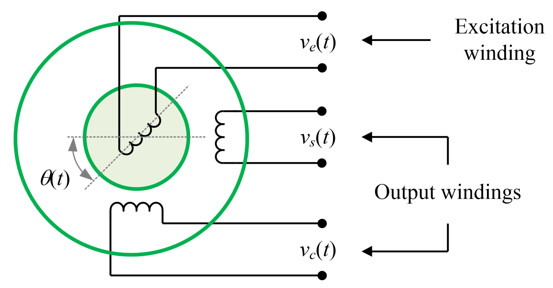
2.1. Resolver

Figure 1 shows the schematics of the resolver. This sensor consists of an excitation winding and two output windings. The excitation winding is coupled to the motor shaft and receives a sinusoidal excitation voltage $v_e\left(t\right)$ of several kHz (1–10 kHz) [21,22,23,24,25,26,27,28]:

$$v_e\left(t\right)=a_{r}cos\left({\omega }_{r}t\right),$$

(1)

where $a_r$ is the excitation voltage amplitude (in V), ${\omega }_r=2\pi f_r$, and $f_r$ is the excitation voltage frequency (in Hz). Two amplitude-modulated voltages $v_s\left(t\right)$ and $v_c\left(t\right)$ are induced in the output windings. Those signals depend on the angular position [24]:

$$v_s\left(t\right)=k_r{v}_e\left(t\right)sin\left(\theta \left(t\right)\right),$$

(2)

$$v_c\left(t\right)=k_r{v}_e\left(t\right)cos\left(\theta \left(t\right)\right).$$

(3)

where $\theta \left(t\right)$ is the angular position to be measured, while $k_r$ is the transformation ratio. The objective of a resolver-to-digital converter (RDC) is to get the angular position from $v_e\left(t\right)$, $v_s\left(t\right)$, and $v_c\left(t\right)$.

2.2. Difference Operation

Let $a\left(k\right)$ and $b\left(k\right)$ be discrete-time signals (vectors or scalars). The first-order difference operator ($\Delta$) and the second-order difference operator (${\Delta }^2$) are defined as follows [50]:

$$\Delta a\left(k\right)=a\left(k\right)-a(k-1),$$

(4)

$${\Delta }^{2}a\left(k\right)=\Delta [\Delta a\left(k\right)]=\Delta a\left(k\right)-\Delta a(k-1).$$

(5)

Let $M_1$ and $M_2$ be matrices such that $M_{1}a\left(k\right)+M_{2}b\left(k\right)$ exists. The aforementioned operators are linear [49,50]:

$$\Delta [M_{1}a\left(k\right)+M_{2}b\left(k\right)]=M_1\Delta a\left(k\right)+M_2\Delta b\left(k\right),$$

(6)

$${\Delta }^2[M_{1}a\left(k\right)+M_{2}b\left(k\right)]=M_1{\Delta }^{2}a\left(k\right)+M_2{\Delta }^{2}b\left(k\right).$$

(7)

The operator $\Delta$ corresponds to the discrete transfer function $C\left(z\right)=1-z^{-1}$ [32].

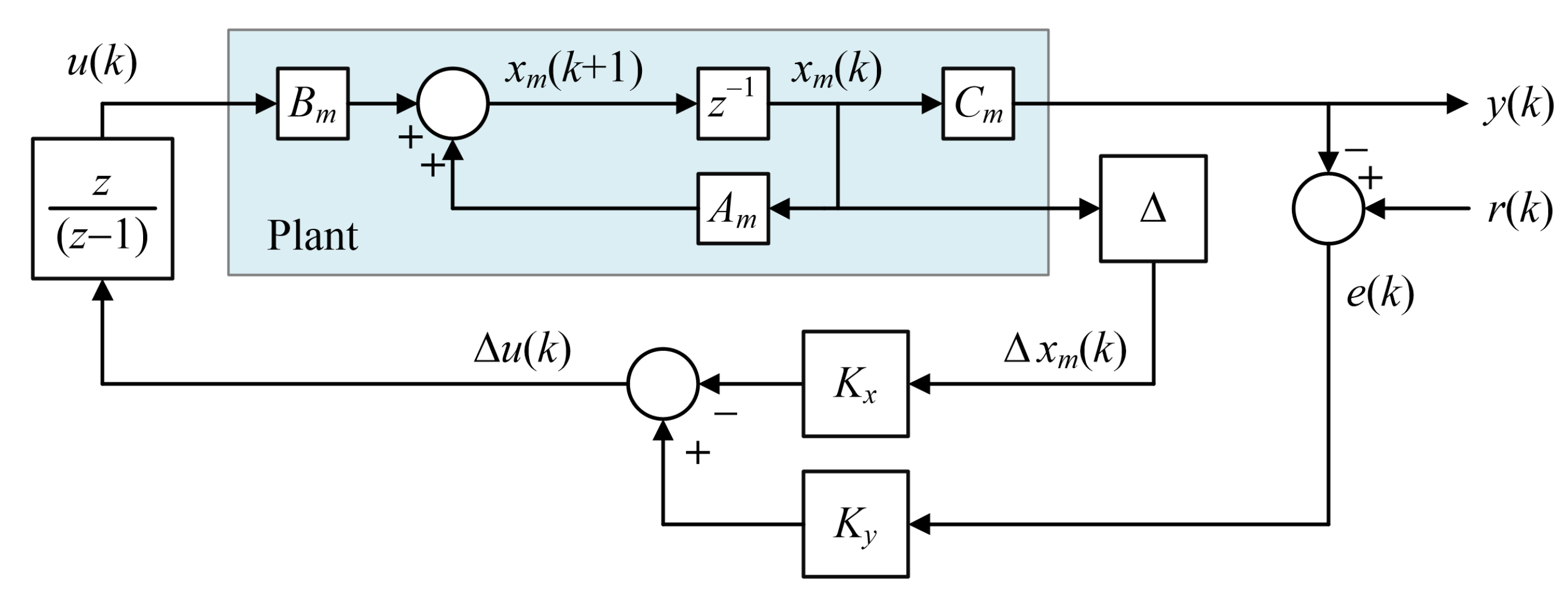
2.3. Conventional GPC

Consider that an n-order SISO (single-input single-output) plant has the following discrete-time space-state model:

$$x_m(k+1)=A_m{x}_m\left(k\right)+B_{m}u\left(k\right),$$

(8)

$$y\left(k\right)=C_m{x}_m\left(k\right),$$

(9)

where $u\left(k\right)$ is the plant input, $y\left(k\right)$ is the system output, $x_m\left(k\right)\in {\Re }^{n\times 1}$ is the plant state vector, while $A_m\in {\Re }^{n\times n}$, $B_m\in {\Re }^{n\times 1}$, and $C_m\in {\Re }^{1\times n}$. Consider that the plant does not have an embedded integrator. The control system must have an integrator so that the steady-state error is zero for a step reference. Conventional GPC requires the development of an augmented model with an embedded integrator. This model will be used to predict plant responses.

Applying the first-order difference operator ($\Delta$) to (8) and (9), based on (6), yields:

$$\begin{array}{ccc}\hfill \Delta x_m(k+1)& =& \Delta [A_m{x}_m\left(k\right)+B_{m}u\left(k\right)]\hfill \\ \hfill & =& A_m\Delta x_m\left(k\right)+B_m\Delta u\left(k\right),\hfill \end{array}$$

(10)

$$\begin{array}{ccc}\hfill \Delta y\left(k\right)& =& \Delta \left[C_m{x}_m\left(k\right)\right]\hfill \\ \hfill & =& C_m\Delta x_m\left(k\right),\hfill \end{array}$$

(11)

where $\Delta x_m\left(k\right)=x_m\left(k\right)-x_m(k-1)$, $\Delta u\left(k\right)=u\left(k\right)-u(k-1)$, and $\Delta y\left(k\right)=y\left(k\right)-y(k-1)$. Note that $y(k+1)=y\left(k\right)+\Delta y(k+1)$ and $y(k+1)=C_m\Delta x_m(k+1)$. Based on these results and (10), $y(k+1)$ is defined in terms of $\Delta x_m\left(k\right)$, $\Delta u\left(k\right)$, and $y\left(k\right)$ [32]:

$$\begin{array}{ccc}\hfill y(k+1)& =& y\left(k\right)+\Delta y(k+1)\hfill \\ \hfill & =& y\left(k\right)+C_m\Delta x_m(k+1)\hfill \\ \hfill & =& y\left(k\right)+C_m{A}_m\Delta x_m\left(k\right)+C_m{B}_m\Delta u\left(k\right).\hfill \end{array}$$

(12)

The augmented model defined in (13) is obtained by placing (10) and (12) together in matrix form [32]:

$$\begin{array}{c}\left[\begin{array}{c}\Delta x_m(k+1)\\ y(k+1)\end{array}\right]=\stackrel{\mathrm{A}}{\overbrace{\left[\begin{array}{cc}{A}_m& o_m^T\\ C_m{A}_m& 1\end{array}\right]}}\stackrel{\mathrm{x}\left(\mathrm{k}\right)}{\overbrace{\left[\begin{array}{c}\Delta x_m\left(k\right)\\ y\left(k\right)\end{array}\right]}}+\stackrel{\mathrm{B}}{\overbrace{\left[\begin{array}{c}{B}_m\\ C_m{B}_m\end{array}\right]}}\Delta u\left(k\right)\\ y\left(k\right)=\stackrel{\mathrm{C}}{\overbrace{\left[\begin{array}{cc}{o}_m& 1\end{array}\right]}}\stackrel{\mathrm{x}\left(\mathrm{k}\right)}{\overbrace{\left[\begin{array}{c}\Delta x_m\left(k\right)\\ y\left(k\right)\end{array}\right]}},\end{array},$$

(13)

where A, B, and C, in (13), are the matrices of the augmented model, while $o_m\in {\Re }^{1\times n}$ is a vector composed of zeros. This augmented model allows predicting the plant responses. Consider that the state vector at instant $k_i$, $x\left(k_i\right)$, is known. The future control trajectory is defined as:

$$\Delta u\left(k_i\right),\Delta u(k_i+1),\cdots ,\Delta u(k_i+N_c-1),$$

(14)

where $N_c$ is a variable called the control horizon. On the other hand, the future state variables are:

$$x(k_i+1|k_i),x(k_i+2|k_i),\cdots ,x(k_i+N_p|k_i),$$

(15)

where $x(k_i+j|k_i)$ is the predicted state vector at instant $k_i+j$ based on $x\left(k_i\right)$, while $N_p$ is the prediction horizon, with $N_c\le N_p$. The value of $N_p$ defines the length of the prediction window [32]. In GPC, the future state variables are predicted using the control future trajectory and $x\left(k_i\right)$ [32]:

$$\begin{array}{c}x(k_i+1|k_i)=Ax\left(k_i\right)+B\Delta u\left(k_i\right),\\ x(k_i+2|k_i)=A^{2}x\left(k_i\right)+AB\Delta u\left(k_i\right)+B\Delta u(k_i+1),\\ ⋮\\ x(k_i+N_p|k_i)=A^{N_p}x\left(k_i\right)+A^{N_p-1}B\Delta u\left(k_i\right)\\ +A^{N_{p}k-2}B\Delta u(k_i+1)+\cdots +A^{N_p-N_c}B\Delta u(k_i+N_c-1).\end{array}$$

(16)

As $y\left(k\right)=C_{m}x\left(k\right)$, the plant outputs are predicted based on (16):

$$\begin{array}{c}y(k_i+1|k_i)=CAx\left(k_i\right)+CB\Delta u\left(k_i\right),\\ y(k_i+2|k_i)=C{A}^{2}x\left(k_i\right)+CAB\Delta u\left(k_i\right)+CB\Delta u(k_i+1),\\ ⋮\\ y(k_i+N_p|k_i)=C{A}^{N_p}x\left(k_i\right)+C{A}^{N_p-1}B\Delta u\left(k_i\right)\\ +C{A}^{N_p-2}B\Delta u(k_i+1)+\cdots +C{A}^{N_p-N_c}B\Delta u(k_i+N_c-1).\end{array}$$

(17)

Putting (17) into a matrix form yields:

$$Y=Fx\left(k_i\right)+\varphi U,$$

(18)

where $Y\in {\Re }^{N_p\times 1}$ is vector with the predicted responses, $U\in {\Re }^{N_c\times 1}$ is the vector with the future control actions, while F and $\varphi$ are defined in (21):

$$Y={\left[\begin{array}{cccc}y(k_i+1|k_i)& y(k_i+2|k_i)& \cdots & y(k_i+N_p|k_i)\end{array}\right]}^T,$$

(19)

$$U={\left[\begin{array}{cccc}\Delta u\left(k_i\right)& \Delta u(k_i+1)& \cdots & \Delta u(k_i+N_c-1)\end{array}\right]}^T,$$

(20)

$$\begin{array}{c}F=\left[\begin{array}{c}CA\\ C{A}^2\\ ⋮\\ C{A}^{N_p}\end{array}\right],\varphi =\left[\begin{array}{cccc}CB& 0& \cdots & 0\\ CAB& CA& \cdots & 0\\ ⋮& ⋮& \cdots & 0\\ C{A}^{N_p-1}& C{A}^{N_p-1}& \cdots & C{A}^{N_p-N_c}\end{array}\right]\end{array}.$$

(21)

Let $r\left(k\right)$ be the reference signal of the plant. The objective of GPC is to calculate an optimal vector of U that minimizes the error between the reference and the predicted plant outputs. Let $R_s\in {\Re }^{N_p\times 1}$ be a vector that contains the references of the predicted responses that composes Y. It is considered that $R_S$ is constant inside the prediction window (the set of predictions) [32]. Equation (22) defines the reference vector $R_s$ according to [32]:

$$R_S^T=\underset{N_p}{\underbrace{\left[\begin{array}{ccc}1& 1& \cdots 1\end{array}\right]}}r\left(k_i\right).$$

(22)

The cost function J, which reflects the control system performance, is defined in [32] as:

$$J={(R_S-Y)}^T(R_S-Y)+U^T{\overline{R}}_{w}U,{\overline{R}}_w=r_w{I}_c,$$

(23)

where $I_c\in {\Re }^{N_c\times N_c}$ is an identity matrix, while $r_w$ is a tuning parameter used to control the magnitude of U [32]. Equation (24) shows the value of $\frac{\partial J}{\partial U}$. The optimal solution of (23) makes $\frac{\partial J}{\partial U}=0$ [32]. By replacing (18) in (24) and after mathematical manipulations, the optimal solution U is defined as indicated in (25) [32]:

$$\frac{\partial J}{\partial U}=-2{\varphi }^T(R_S-Fx\left(k_i\right))+2({\varphi }^T\varphi +{\overline{R}}_w)U=0.$$

(24)

$$U={({\varphi }^T\varphi +{\overline{R}}_w)}^{-1}{\varphi }^T(R_S-Fx\left(k_i\right)).$$

(25)

According to receding horizon approach, only the first element of the optimal control trajectory, i.e., $\Delta u\left(k_i\right)$,is used to calculate the control law [32]. Thus:

$$\begin{array}{ccc}\hfill \Delta u\left(k_i\right)& =& \stackrel{N_c}{\overbrace{\left[\begin{array}{ccc}1& 0& \cdots 0\end{array}\right]}}{({\varphi }^T\varphi +{\overline{R}}_w)}^{-1}({\varphi }^T{R}_S-{\varphi }^{T}Fx\left(k_i\right))\hfill \\ \hfill & =& K_{y}r\left(k_i\right)-K_{mpc}x\left(k_i\right),\hfill \end{array}$$

(26)

where $K_y$ is the first element of ${({\varphi }^T\varphi +{\overline{R}}_w)}^{-1}\left({\varphi }^T{R}_S\right)$ and $K_{mpc}$ is the first line of ${({\varphi }^T\varphi +{\overline{R}}_w)}^{-1}\left({\varphi }^{T}Fx\left(k_i\right)\right)$. The gain vector $K_{mpc}$ can be expressed as $K_{mpc}=\left[K_x{K}_y\right]$, where $K_y\in {\Re }^{1\times 1}$ is the last element of $K_{mpc}$, while $K_x\in {\Re }^{n\times 1}$. Based on (26) and the definition of $x\left(k\right)$ in (13), it is possible to prove [32]:

$$\Delta u\left(k_i\right)=K_y(r\left(k_i\right)-y\left(k_i\right))-K_x\Delta x_m\left(k_i\right).$$

(27)

The closed-loop GPC system described in [32] can be described as shown in Figure 2, where the $z^{-1}$ block indicates the discrete delay operator, $1-z^{-1}$ is the discrete transfer function equivalent to the $\Delta$ operator, while $\frac{1}{1-z^{-1}}$ corresponds to the discrete-time integrator. The plant input is obtained by integrating $\Delta u\left(k_i\right)$ in (27).

3. Proposed RDC System Based on SOD-GPC

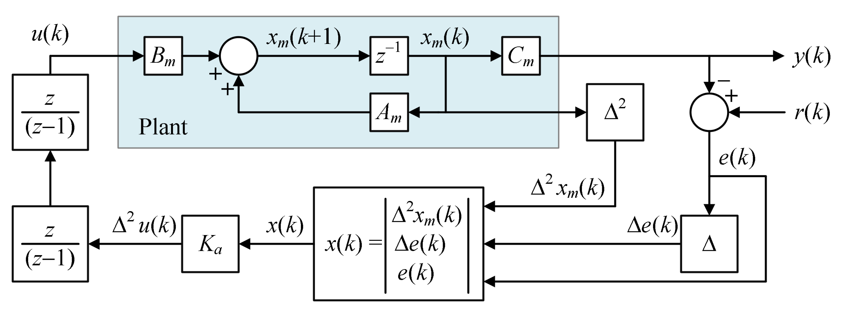
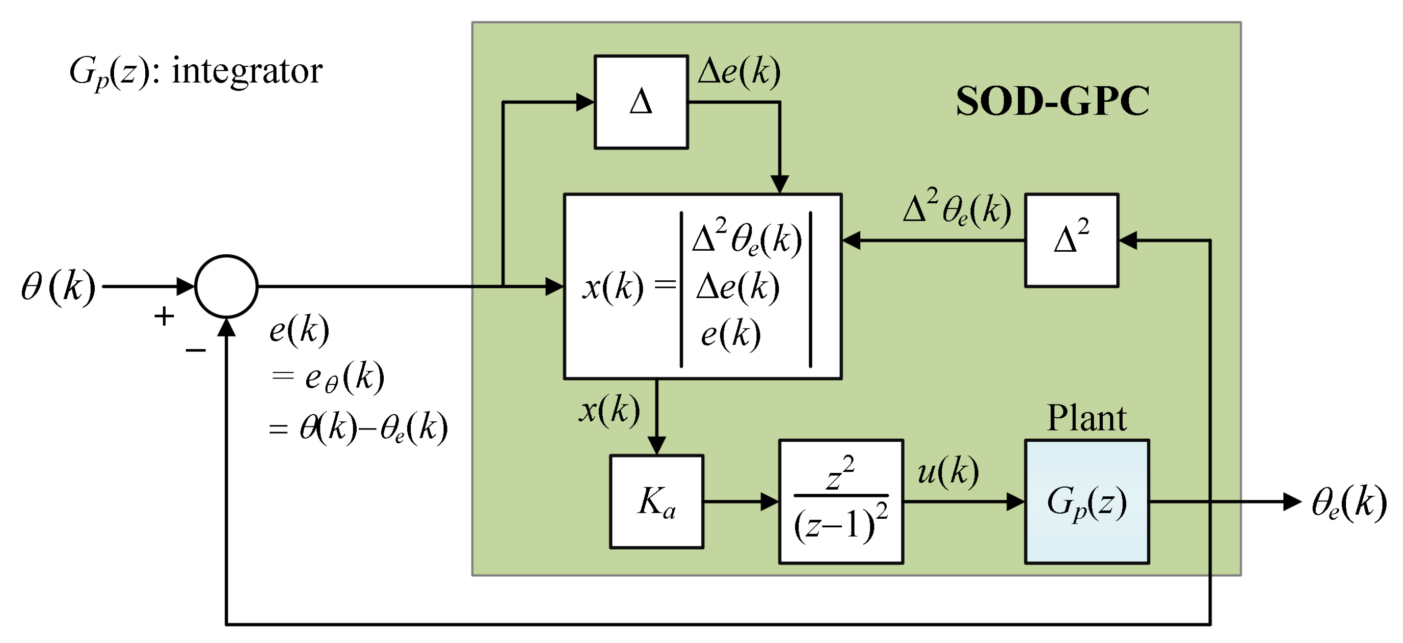
3.1. Second-Order Difference GPC

According to the internal model principle, if the plant has no integrator, then the controller must have two embedded integrators to track ramp references [46]. However, the conventional GPC approach in [32] only has one embedded integrator. Besides, the cost function of the GPC described in (23) considers that the prediction window reference vector ($R_S$) is constant within the prediction window [32]. However, the reference vector defined in (22) is not constant when the plant reference $r\left(k\right)$ is a ramp signal.

Cordero et al. proposed in [49] an adaptation of the GPC algorithm for reference tracking. This approach is based on applying the second-order difference operator in (4) to create an augmented model with two embedded integrators and whose output is the tracking error. For the sake of simplicity, the GPC approach in [49] will be called second-order difference GPC (SOD-GPC) in this paper.

Applying the second-order difference operator in (8), as this operator is linear, yields:

$${\Delta }^2{x}_m(k+1)=C_m{A}_m{\Delta }^2{x}_m\left(k\right)+C_m{B}_m{\Delta }^{2}u\left(k\right).$$

(28)

Let $e\left(k\right)$ be the tracking error:

$$e\left(k\right)=r\left(k\right)-y\left(k\right).$$

(29)

Hence:

$$e(k+1)=r(k+1)-y(k+1).$$

(30)

Applying the first-order difference operator to (12), (29), and (30) yields [49]:

$$\Delta e\left(k\right)=\Delta r\left(k\right)-\Delta y\left(k\right),$$

(31)

$$\Delta e(k+1)=\Delta r(k+1)-\Delta y(k+1),$$

(32)

$$\begin{array}{cc}\hfill \Delta y(k+1)& =\Delta \left[y\left(k\right)+C_m{A}_m\Delta x_m\left(k\right)+C_m{B}_m\Delta u\left(k\right)\right]\\ \hfill & =\Delta y\left(k\right)+C_m{A}_m{\Delta }^2{x}_m\left(k\right)+C_m{B}_m{\Delta }^{2}u\left(k\right).\end{array}$$

(33)

On the other hand, let $r\left(k\right)=\alpha k+\beta$ be the ramp reference signal. Observe that $\Delta r\left(k\right)=r\left(k\right)-r(k-1)=\alpha$. $\Delta r(k+1)=r(k+1)-r\left(k\right)=\alpha$. Therefore:

$$\Delta r(k+1)=\Delta r\left(k\right).$$

(34)

Replacing (31), (33), and (34) in (32) yields:

$$\begin{array}{ccc}\hfill \Delta e(k+1)& =& \Delta r\left(k\right)-\left[\Delta y\left(k\right)+C_m{A}_m{\Delta }^2{x}_m\left(k\right)+C_m{B}_m{\Delta }^{2}u\left(k\right)\right]\hfill \\ \hfill & =& \Delta e\left(k\right)-C_m{A}_m{\Delta }^2{x}_m\left(k\right)-C_m{B}_m{\Delta }^{2}u\left(k\right).\hfill \end{array}$$

(35)

Observe that $\Delta e(k+1)=e(k+1)-e\left(k\right)$. Hence:

$$e(k+1)=e\left(k\right)+\Delta e(k+1).$$

(36)

Replacing (35) in (36) yields:

$$\begin{array}{ccc}\hfill e(k+1)& =& e\left(k\right)+\Delta e(k+1)\hfill \\ \hfill & =& e\left(k\right)+\Delta e\left(k\right)-C_m{A}_m{\Delta }^2{x}_m\left(k\right)-C_m{B}_m{\Delta }^{2}u\left(k\right).\hfill \end{array}$$

(37)

The augmented model proposed defined in (38) is obtained from (28), (35), and (37) [49]:

$$\begin{array}{c}x(k+1)=A_{2}x\left(k\right)+B_2{\Delta }^{2}u\left(k\right),\\ \mathrm{Output}\text{:}e\left(k\right)=C_{2}x\left(k\right),\end{array}$$

(38)

where:

$$\begin{array}{c}x\left(k\right)=\left[\begin{array}{c}{\Delta }^2{x}_m\left(k\right)\\ \Delta e\left(k\right)\\ e\left(k\right)\end{array}\right],A_2=\left[\begin{array}{ccc}{A}_m& o_o^T& o_o^T\\ -C_m{A}_m& 1& o_o^T\\ -C_m{A}_m& 1& 1\end{array}\right],B_2=\left[\begin{array}{c}{B}_m\\ -C_m{B}_m\\ -C_m{B}_m\end{array}\right],\\ C_2=\left[\begin{array}{ccc}{o}_o& 0& 1\end{array}\right].\end{array}$$

(39)

Note that the input and the output of (38) are ${\Delta }^{2}u\left(k\right)$ and $e\left(k\right)$, respectively. In [49], the prediction window is composed by the predicted tracking errors $e(k_i+1|k_i),e(k_i+2|k_i),\cdots ,e(k_i+N_p|k_i)$, while the future control trajectory is ${\Delta }^{2}u\left(k_i\right),{\Delta }^{2}u(k_i+1),\cdots ,{\Delta }^{2}u(k_i+N_c-1)$. Thus, the vector with the predicted response ($Y_a$) and the vector with the future control signals ($U_a$) for the SOD-GPC system proposed in [49] are defined as follows:

$$Y_a={\left[\begin{array}{cccc}e(k_i+1|k_i)& e(k_i+2|k_i)& \cdots & e(k_i+N_p|k_i)\end{array}\right]}^T,$$

(40)

$$U_a={\left[\begin{array}{cccc}{\Delta }^{2}u\left(k_i\right)& {\Delta }^{2}u(k_i+1)& \cdots & {\Delta }^{2}u(k_i+N_c-1)\end{array}\right]}^T.$$

(41)

The proposed augmented model in (38) has a similar structure as the GPC augmented model in (13). Thus, it is possible to apply the method defined in (18) to predict the tracking error (the outputs of the augmented mode) in (38):

$$Y_a=Fx\left(k_i\right)+\varphi U_a,$$

(42)

where F and $\varphi$ are defined in (21), but replacing the matrices A, B, and C with $A_2$, $B_2$, and $C_2$ in (39), respectively.

Observe that the desired values of the predicted errors that compose $Y_a$ are zero. Therefore, the reference vector is a set of zeros, i.e., $R_S=0$, which is constant. Replacing Y, U, and $R_S$ with $Y_a$, $U_a$, and 0 in (23) and (24) yields [49]:

$$J=Y_a^T{Y}_a+U_a^T{\overline{R}}_w{U}_a,$$

(43)

$$\frac{\partial J}{\partial U_a}=2{\varphi }^{T}Fx\left(k_i\right)+2({\varphi }^T\varphi +{\overline{R}}_w)U_a=0.$$

(44)

The optimal solution $U_a$ for the SOD-GPC makes $\frac{\partial J}{\partial U_a}=0$ in (44). This solution is:

$$U_a=-{({\varphi }^T\varphi +{\overline{R}}_w)}^{-1}{\varphi }^{T}Fx\left(k_i\right).$$

(45)

Equation (45) defines the optimal control trajectory of the SOD-GPC. According to the receding horizon control principle, only the first element of $U_a$ in (45), i.e., ${\Delta }^{2}u\left(k_i\right)$, is used to calculate the control law. Thus:

$${\Delta }^{2}u\left(k_i\right)=-\stackrel{N_c}{\overbrace{\left[\begin{array}{ccc}1& 0& \cdots 0\end{array}\right]}}{({\varphi }^T\varphi +{\overline{R}}_w)}^{-1}{\varphi }^{T}Fx\left(k_i\right).$$

(46)

The plant input is obtained by integrating ${\Delta }^{2}u\left(k_i\right)$ in (46) twice. Figure 3 shows the structure of the SOD-GPC system described in [49]. The dynamics of the control system depends on the tuning of $N_p$, $N_c$, and ${\overline{R}}_w$.

$$\Delta u\left(k_i\right)={\Delta }^{2}u\left(k_i\right)+\Delta u(k_i-1),u\left(k_i\right)=\Delta u\left(k_i\right)+u(k_i-1).$$

(47)

Let $G\left(z\right)$ and $G_a\left(z\right)$ be the plant’s discrete transfer functions and the SOD-GPC augmented model. It was proven in [49]:

$$G_a=-{\left[\begin{array}{c}\frac{z}{z-1}\end{array}\right]}^{2}G\left(z\right).$$

(48)

Equation (48) proves that the augmented model in (38) has two embedded integrators, when the plant has no zeros at $z=1$. Hence, the SOD-GPC can asymptotically track the ramp references [49].

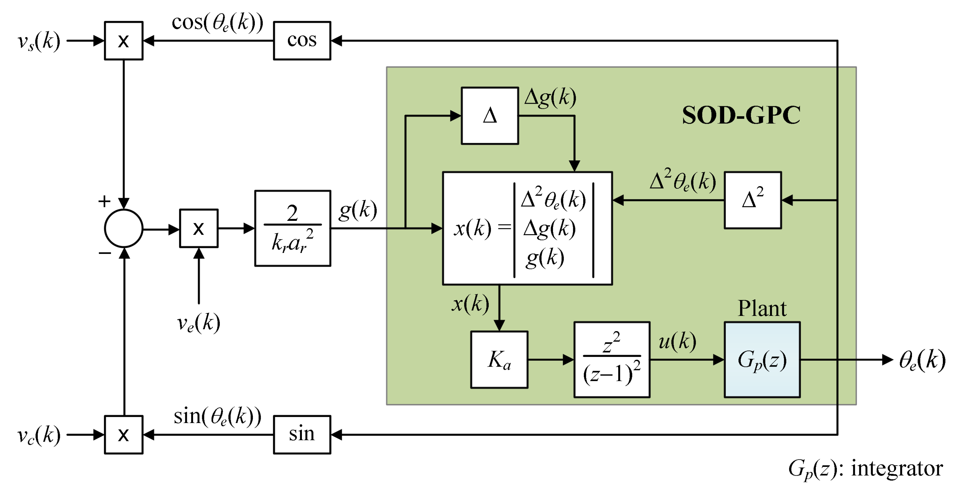
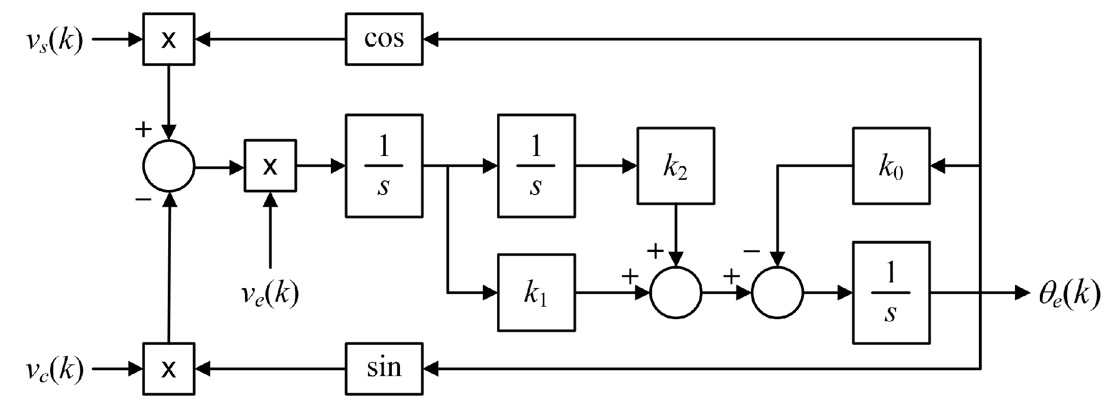
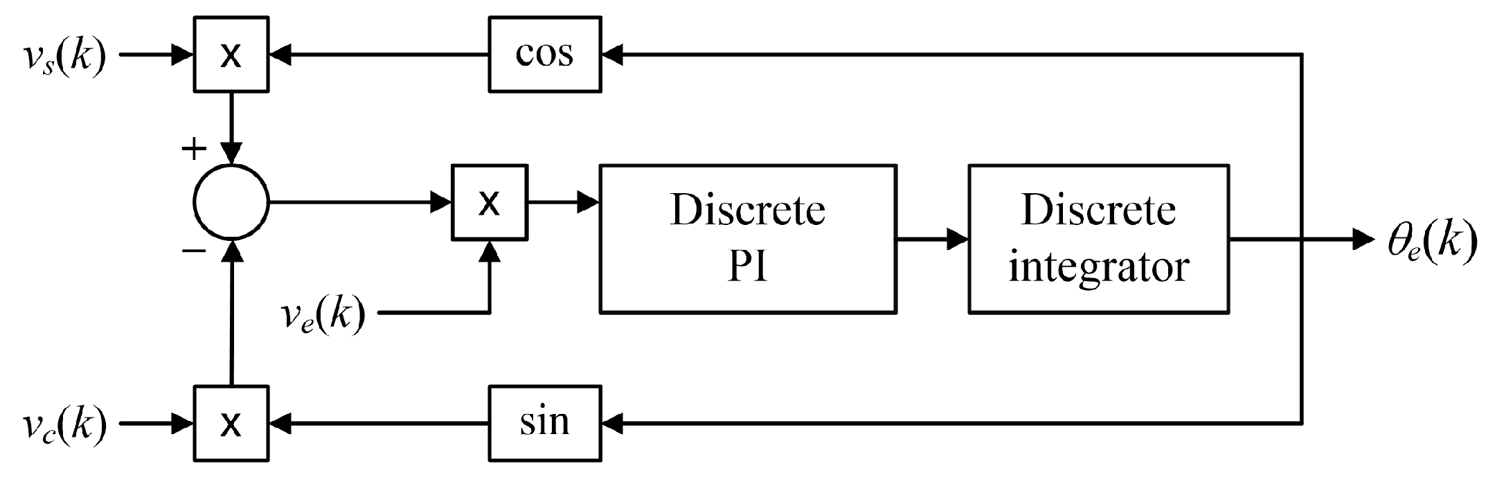
3.2. Proposed GPC-Based ATO

Figure 4 shows the structure of the proposed ATO based on the SOD-GPC. Consider that the resolver excitation signal with frequency ${\omega }_r=2\pi f_r$ is generated by the RDC. Thus, the value of this signal is known. Let $t=t_{s}k$, where t is the discretized time, $t_s$ is the sampling time, $f_s=\frac{1}{t_s}$ is the sampling frequency, while k denotes the k-th sample. Define ${\omega }_{rs}$ as the normalized resolver excitation frequency:

$${\omega }_{rs}={\omega }_r{t}_s=\frac{2\pi f_r}{f_s}.$$

(49)

Let $\theta \left(k\right)=\theta \left(k{t}_s\right)$ and ${\theta }_e\left(k\right)={\theta }_e\left(k{t}_s\right)$ be the actual and estimated angles. Thus, based on (49), the resolver signals in (1)–(3) can be discretized as follows:

$$\begin{array}{ccc}\hfill v_e\left(k\right)& =& a_{r}cos\left({\omega }_r{t}_{s}k\right)=a_{r}cos\left({\omega }_{rs}k\right),\hfill \end{array}$$

(50)

$$\begin{array}{ccc}\hfill v_s\left(k\right)& =& k_r{v}_e\left(k\right)sin\left(\theta \left(k\right)\right),\hfill \end{array}$$

(51)

$$\begin{array}{ccc}\hfill v_c\left(k\right)& =& k_r{v}_e\left(k\right)cos\left(\theta \left(k\right)\right),\hfill \end{array}$$

(52)

According to Figure 4, the term $g\left(k\right)$ is:

$$g\left(k\right)={\displaystyle \frac{2}{k_r{a}_r^2}}\left[v_s\left(k\right)cos\left({\theta }_e\left(k\right)\right)-v_c\left(k\right)sin\left({\theta }_e\left(k\right)\right)\right]v_e\left(k\right).$$

(53)

Replacing (50)–(52) in (53) and applying trigonometry yield:

$$\begin{array}{ccc}\hfill g\left(k\right)& =& {\displaystyle \frac{2}{k_r{a}_r^2}}\left[k_r{v}_e\left(k\right)sin\left(\theta \left(k\right)\right)cos\left({\theta }_e\left(k\right)\right)-k_r{v}_e\left(k\right)cos\left(\theta \left(k\right)\right)sin\left({\theta }_e\left(k\right)\right)\right]v_e\left(k\right)\hfill \\ \hfill & =& {\displaystyle \frac{2}{a_r^2}}\left[sin\left(\theta \left(k\right)\right)cos\left({\theta }_e\left(k\right)\right)-cos\left(\theta \left(k\right)\right)sin\left({\theta }_e\left(k\right)\right)\right]v_e^2\left(k\right)\hfill \\ \hfill & =& {\displaystyle \frac{2}{a_r^2}}sin(\theta \left(k\right)-{\theta }_e\left(k\right))a_r^{2}co{s}^2\left({\omega }_{rs}k\right)\hfill \\ \hfill & =& sin\left(e_{\theta }\left(k\right)\right)\left[1+cos\left(2{\omega }_{rs}k\right)\right]\hfill \\ \hfill & =& sin\left(e_{\theta }\left(k\right)\right)+sin\left(e_{\theta }\left(k\right)\right)cos\left(2{\omega }_{r}k\right),\hfill \end{array}$$

(54)

where $e_{\theta }\left(k\right)=\theta \left(k\right)-{\theta }_e\left(k\right)$ is the angle estimation error, and assuming that $e_{\theta }\left(k\right)\approx 0$, then $sin\left(e_{\theta }\left(k\right)\right)\approx e_{\theta }\left(k\right)$. Thus, (54) is rewritten as follows:

$$g\left(k\right)\approx e_{\theta }\left(k\right)+e_{\theta }\left(k\right)cos\left(2{\omega }_{rs}k\right).$$

(55)

Let $Z\left[s\right(k\left)\right]$ denote the Z-transform of the discrete signal $s\left(k\right)$. Let $H\left(z\right)$ be the transfer function of the SOD-GPC system (including the integrator $G_p\left(z\right)$) shown in Figure 4. $H\left(z\right)$ represents the relationship between $Z\left[{\theta }_e\left(k\right)\right]$ and $Z\left[g\right(k\left)\right]$, i.e., $H\left(z\right)=\frac{Z\left[{\theta }_e\left(k\right)\right]}{Z\left[g\right(k\left)\right]}$. Let $h\left(k\right)$ be the impulse response of the SOD-GPC system, i.e., $Z\left[h\right(k\left)\right]=H\left(z\right)$. Hence [51]:

$$Z\left[{\theta }_e\left(k\right)\right]=H\left(z\right)Z\left[g\left(k\right)\right]\to {\theta }_e\left(k\right)=h\left(k\right)\ast g\left(k\right),$$

(56)

where * denotes convolution. As the SOD-GPC is a linear system, it is possible to apply the superposition principle to analyze the ATO response: the estimated angular position (the ATO output) is the summation of the responses produced by $e_{\theta }\left(k\right)$ and $e_{\theta }\left(k\right)cos\left(2{\omega }_{rs}k\right)$:

$$\begin{array}{ccc}\hfill {\theta }_e\left(k\right)& =& h\left(k\right)\ast g\left(k\right)\hfill \\ \hfill & =& h\left(k\right)\ast \left[e_{\theta }\left(k\right)+e_{\theta }\left(k\right)cos\left(2{\omega }_{rs}k\right)\right]\hfill \\ \hfill & =& h\left(k\right)\ast e_{\theta }\left(k\right)+h\left(k\right)\ast \left[e_{\theta }\left(k\right)cos\left(2{\omega }_{rs}k\right)\right].\hfill \end{array}$$

(57)

Through the frequency shifting property, it is possible to prove that the term $e_{\theta }\left(k\right)cos\left(2{\omega }_{rs}k\right)$ is a high-frequency signal, while the ATO acts as a low-pass filter that rejects high-frequency signals [28]. As a result, the effect of the signal $e_{\theta }\left(k\right)cos\left(2{\omega }_{rs}k\right)$ in the angle estimation will be rejected by the ATO:

$$h\left(k\right)\ast \left[e_{\theta }\left(k\right)cos\left(2{\omega }_{rs}k\right)\right]\approx 0.$$

(58)

Replacing (58) in (57) yields:

$${\theta }_e\left(k\right)\approx h\left(k\right)\ast e_{\theta }\left(k\right).$$

(59)

Equation (59) states that the estimated angle mainly depends on the term $e_{\theta }\left(k\right)$. As a consequence, the ATO can be projected only considering the existence of $e_{\theta }\left(k\right)$. Thus, the ATO can be approximated as the closed-loop system in Figure 5, where the reference is $\theta \left(k\right)$, the output is ${\theta }_e\left(k\right)$, and the SOD-GPC is the controller that reduce the error $e_{\theta }\left(k\right)$. The plant whose output will be defined by the SOD-GPC algorithm is the integrator represented by $G_p\left(z\right)$ in Figure 5. An ATO is an observer that estimates the angular position. However, many approaches in the literature model the ATO as a closed-loop system whose objective is to reduce the angle estimation error [24,27,28,45]. In the proposed ATO, the angle estimation error is obtained from the signal $g\left(k\right)$. The discrete-time model of the integrator is described through (8) and (9), where $A_m=1$, $B_m=t_s$, $C_m=1$, and $y\left(k\right)=x_m\left(k\right)={\theta }_e\left(k\right)$. The closed-loop error ($e\left(k\right)$) is the angle estimation error, i.e., $e\left(k\right)=e_{\theta }\left(k\right)$. Replacing these terms in (39) yields:

$$\begin{array}{c}x\left(k\right)=\left[\begin{array}{c}{\Delta }^2{\theta }_e\left(k\right)\\ \Delta e\left(k\right)\\ e\left(k\right)\end{array}\right],A_2=\left[\begin{array}{ccc}1& 0& 0\\ -1& 1& 0\\ -1& 1& 1\end{array}\right],B_2=\left[\begin{array}{c}{t}_s\\ -t_s\\ -t_s\end{array}\right],C_2=\left[\begin{array}{ccc}0& 0& 1\end{array}\right].\end{array}$$

(60)

The matrices A, B, and C in (60) must be used to obtain the gain matrix $K_a$ and the control law according to (21), (46), and (47). The adequate tuning of the parameters $N_p$, $N_c$, and ${\overline{R}}_w$ is required to define the transient behavior of the ATO.

As $G_p\left(z\right)$ in Figure 4 is an integrator, then the integral of $u\left(k\right)$ is the estimated position ${\theta }_e\left(k\right)$. Hence, the signal $u\left(k\right)$ produced by the SOD-GPC system is the estimated angular speed. However, if the noise power in the resolver signals is high, $u\left(k\right)$ should be filtered to get a good speed estimation (the design of that filter is beyond the objectives of this research). As a result, the proposed ATO allows estimating the angular speed.

3.3. Effect of Resolver Parameter Variations in the Angle Estimation

Equations (2) and (3) are the ideal representation of the resolver outputs. However, imperfections in the mechanical resolver structure and the signal conditioning circuits introduce distortions to the resolver outputs [52,53,54,55]. The main distortions that affect the angle estimation are:

• Amplitude imbalance: amplitude difference between the resolver outputs.
• Imperfect quadrature: spatial misalignment between the two resolver phases.

Other distortions, such as DC offset in the envelopes of the resolver outputs and harmonics, have a small effect [52,53,54,55]. The resolver outputs can be modeled, considering the effects of the amplitude imbalance and the imperfect quadrature, as follows:

$$v_s\left(t\right)=k_r{v}_e\left(t\right)sin(\theta \left(t\right)+\beta ),$$

(61)

$$v_c\left(t\right)=(1+\alpha )k_r{v}_e\left(t\right)cos\left(\theta \left(t\right)\right).$$

(62)

where $\alpha$ and $\beta$ are, respectively, the amount of amplitude imbalance and imperfect quadrature error. These distortions produce low-frequency angle estimation errors [52,53,54,55]. The compensation of the resolver imperfection effects is beyond the objective of this research. However, many calibration techniques have been proposed in the literature to measure and compensate these distortions, which can be applied with the proposed ATO [52,53,54,55].

4. Results

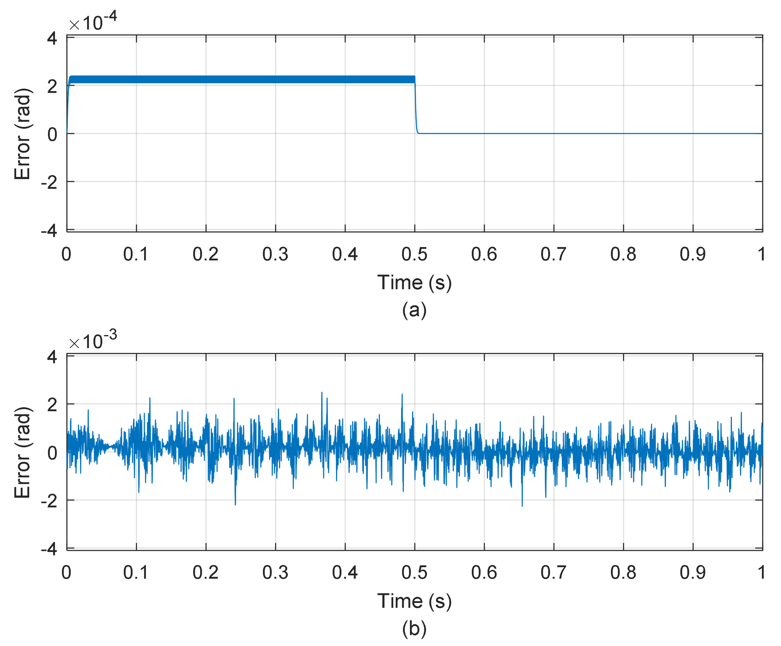
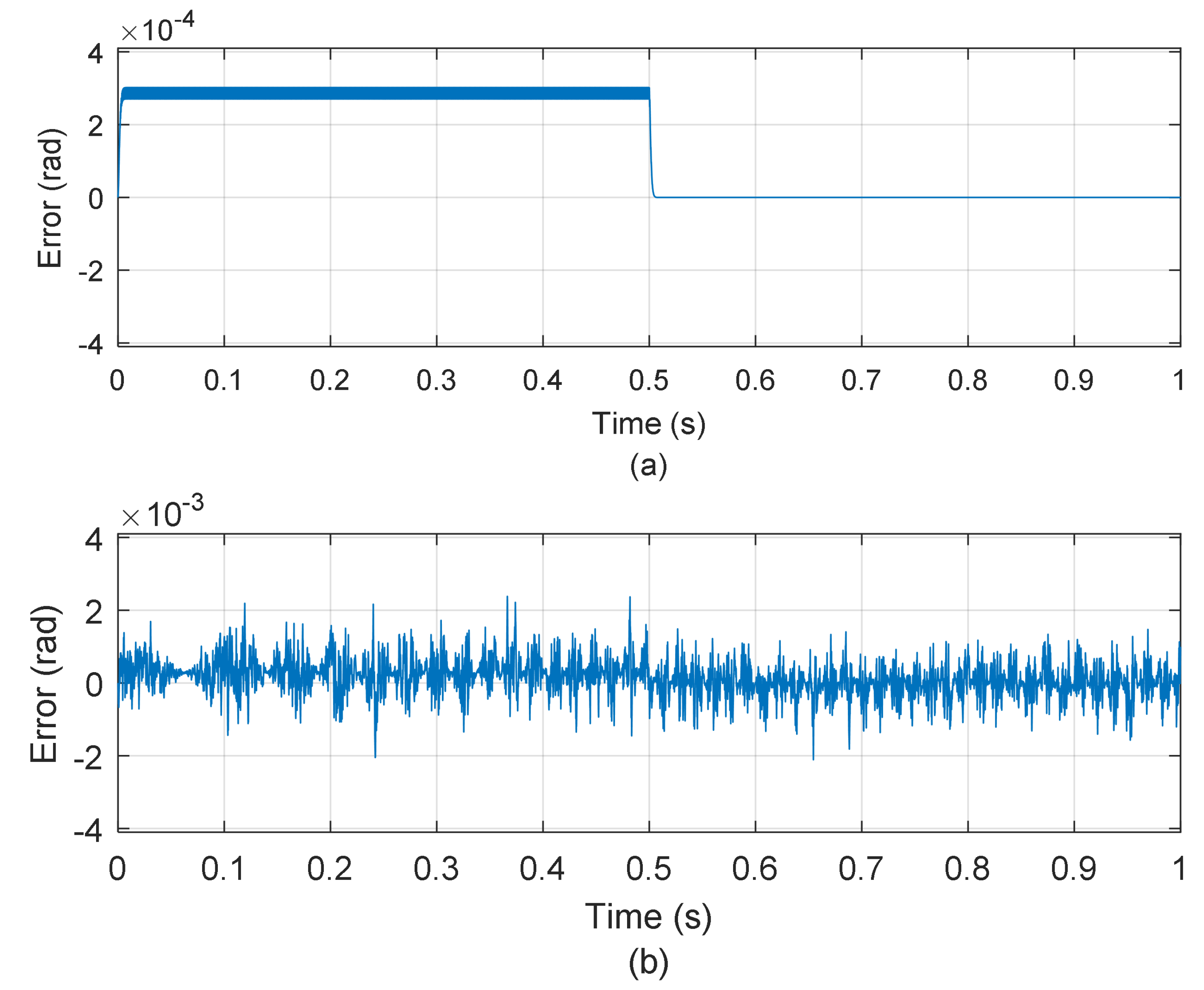
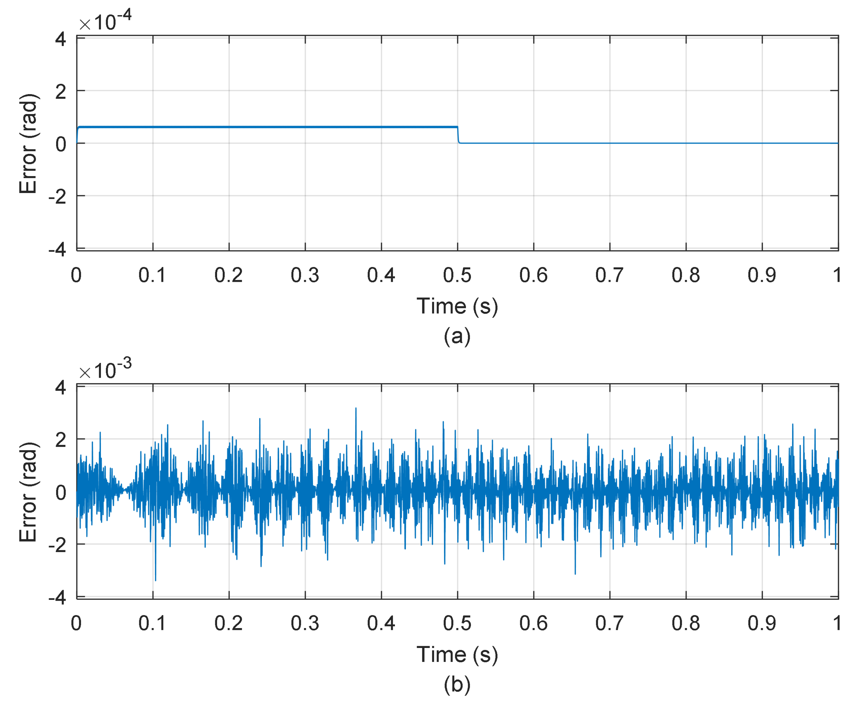
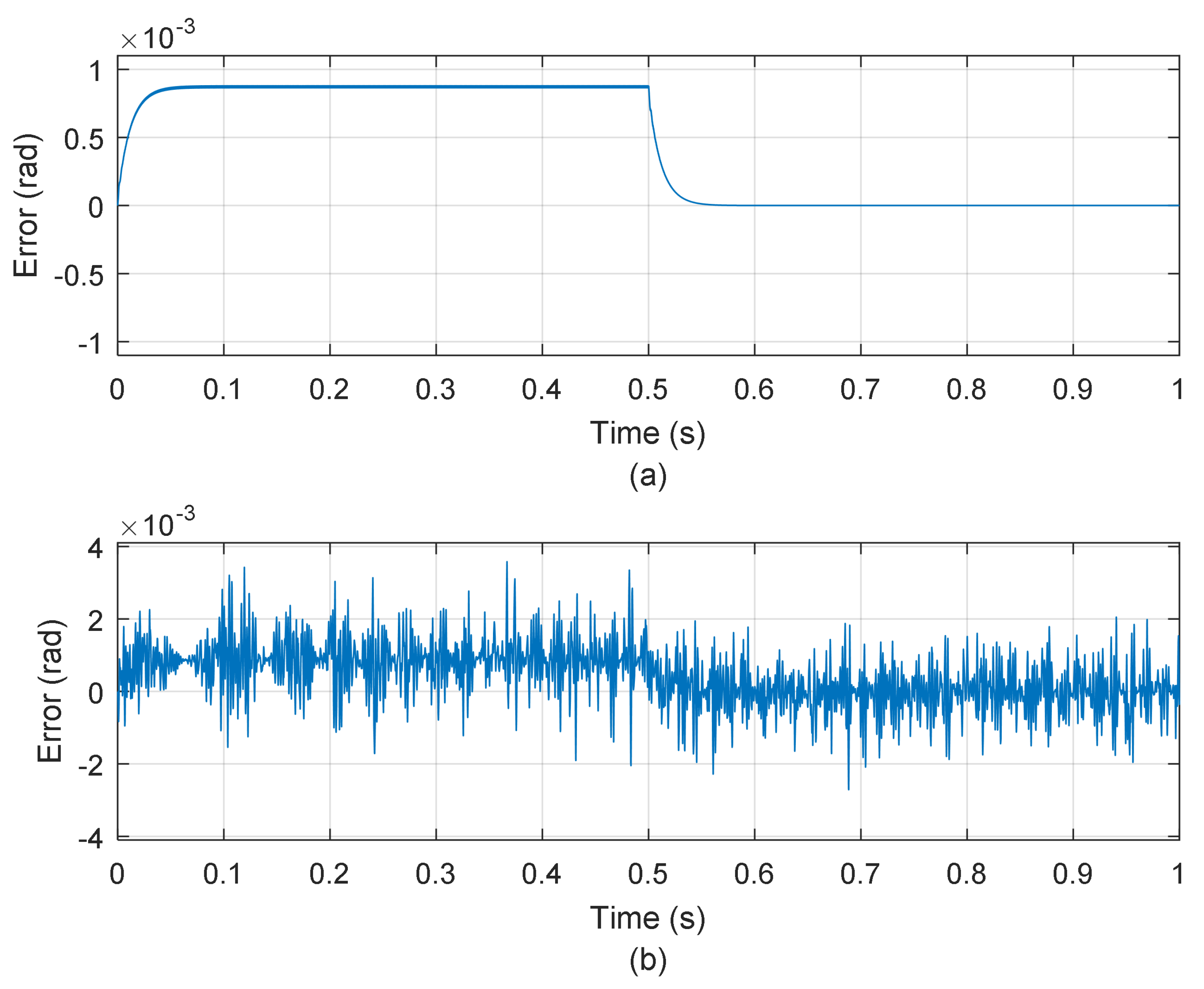
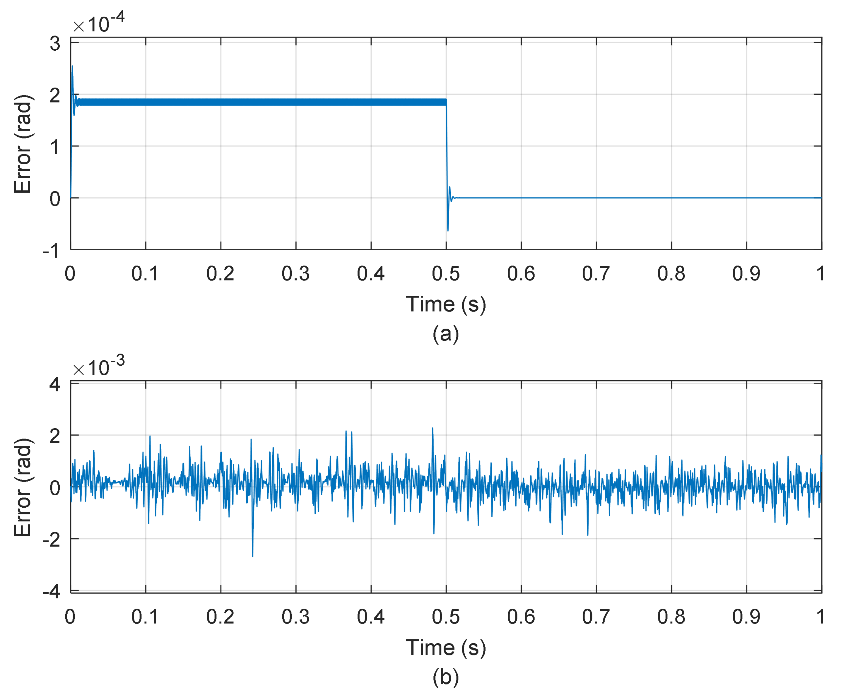
4.1. Simulation Results

A set of simulation tests was performed in MATLAB/Simulink. The sampling rate was set at 50 kHz. The parameters of the resolver sensor are listed in

Table 1. Simulation parameters of the resolver sensor.

Parameters	Values
Excitation amplitude ($a_r$)	8 V
Excitation frequency ($f_r$)	2.5 kHz
Transformation ratio ($k_r$)	0.5

. The angular position corresponds to the speed curve shown in Figure 6. The proposed ATO was tested considering different values of $N_p$, $N_c$, and ${\overline{R}}_w$:

• Configuration 1: $N_p=102,N_c=2,{\overline{R}}_w=0.01$,
• Configuration 2: $N_p=120,N_c=2,{\overline{R}}_w=0.01$,
• Configuration 3: $N_p=102,N_c=10,{\overline{R}}_w=0.01$.

The proposed approach was compared with the ATO described in [56], and with an ATO where the SOD-GPC was replaced by a PI controller (PI-based ATO). Figure 7 and Figure 8 illustrate the ATO in [56] and the PI-based ATO, respectively. The dynamic behavior of the ATO in Figure 7 depends on the solutions (${\lambda }_i$) of the equation $({\lambda }_{i}I-M)=0$, where ${\lambda }_i$ is the i-th eigenvalue of M, $i=1,2,3$, I is the identity matrix, while $M=\left[\begin{array}{ccc}0& 0& 0\\ -1& 0& 0\\ 0& 1& 0\end{array}\right]-\left[\begin{array}{c}0.5{\left(k_r{a}_r\right)}^2\\ 0\\ 0\end{array}\right]\underset{K}{\underbrace{[k_0-k_1-k_2]}}$. The Ackermann formula was used to get the matrix K to set the eigenvalues of M. In this paper, those eigenvalues were set as $-100+j100$, $-100-j100$, and $-500$. These eigenvalues were selected after many simulations, trying to get a response similar to the proposed ATO. Observe that the complex-conjugate eigenvalues are dominant. The application of complex-conjugate eigenvalues to tune an ATO can be found in [28]. On the other hand, the PI regulator of the PI-based ATO in Figure 8 has the discrete transfer function $C\left(z\right)=\frac{500.52\times (z-0.957)}{z-1}$. The PID tuning tool of MATLAB was used to set the parameters of the PI in order for the PI-based ATO and the proposed ATO to have a similar response. A sampling rate of 50 kHz was used for the discretization process. To avoid algebraic loops in the ATO models, each integrator whose output was the estimated angle was discretized through forward Euler approximation. In contrast, backward Euler approximation was used to implement the other integrators.

Table 2. Computational cost of ATOs.

ATO	Sum (+)	Multiplication (×)
SOD-GPC-based ATO	9	8
ATO in [56]	6	9
PI-based ATO	3	6

shows the number of multiplications and sums necessary to implement the SOD-GPC-based ATO, the ATO in [56], and the PI-based ATO, without considering the estimation of the trigonometric functions. The multiplication operation has a longer processing time than the sum operator. Table 2 shows that the SOD-GPC has eight multiplication operators in its structure, two more than the PI-based ATO, which is a low computational cost system due to the modeling’s simplicity. On the other hand, the proposed ATO uses less multiplications than the ATO in [56]. The SOD-GPC uses one matrix multiplication, two accumulators $\left(\frac{z}{z-1}\right)$ (an accumulator uses only one sum), and the estimation of the difference operators (subtractions). As a result, the SOD-GPC has low complexity, and it can be easily implemented.

For each ATO configuration, two tests were performed: without adding noise to the resolver outputs and adding noise (zero mean and 0.0002 variance) to the resolver outputs. Figure 9, Figure 10, Figure 11, Figure 12 and Figure 13 show the angle estimation error for each simulation test.

Table 3. RMSE and settling time in the simulation tests.

Configuration	RMSE (without Noise)	RMSE (with Noise)	Settling Time (s)
$N_p=102,N_c=2,{\overline{R}}_w=0.01$	$0.16\times {10}^{-3}$	$0.48\times {10}^{-3}$	$4.90\times {10}^{-3}$
$N_p=120,N_c=2,{\overline{R}}_w=0.01$	$0.20\times {10}^{-3}$	$0.47\times {10}^{-3}$	$5.10\times {10}^{-3}$
$N_p=102,N_c=10,{\overline{R}}_w=0.01$	$0.04\times {10}^{-3}$	$0.68\times {10}^{-3}$	$2.10\times {10}^{-3}$
ATO in [56]	$0.61\times {10}^{-3}$	$0.88\times {10}^{-3}$	$55.0\times {10}^{-3}$
PI-based ATO	$0.14\times {10}^{-3}$	$0.45\times {10}^{-3}$	$22.3\times {10}^{-3}$

shows the root mean squared error (RMSE) and the error settling time (the time required for the error signal to achieve its steady-state value) for each simulation test. The errors without noise are negligible in all cases. Thus, the main source of angular estimation error is the noise in the resolver outputs. As a result, the value of the RMSE is a measurement of the robustness against noise of the ATO: the lesser the value of RMSE, the better the ATO robustness against noise. According to Table 3, it is possible to see that the ATO in [56] has a higher RMSE and settling time than the proposed approach. As a result, the proposed RDC based on the SOD-GPC has a faster response and greater robustness against noise than the approach in [56]. Besides, the settling time for the proposed ATO is less than the value obtained for the PI-based ATO (both ATOs have similar RMSEs).

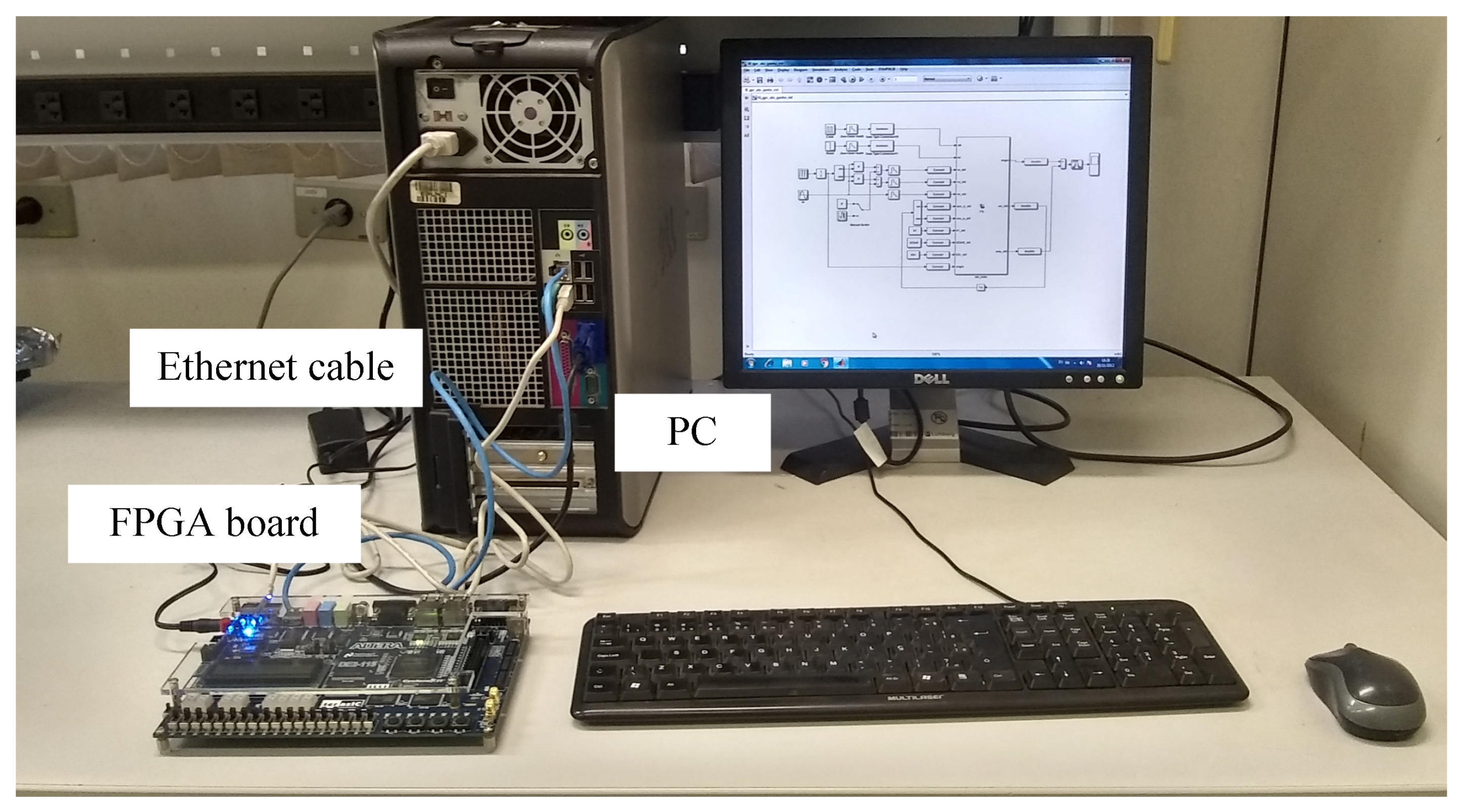
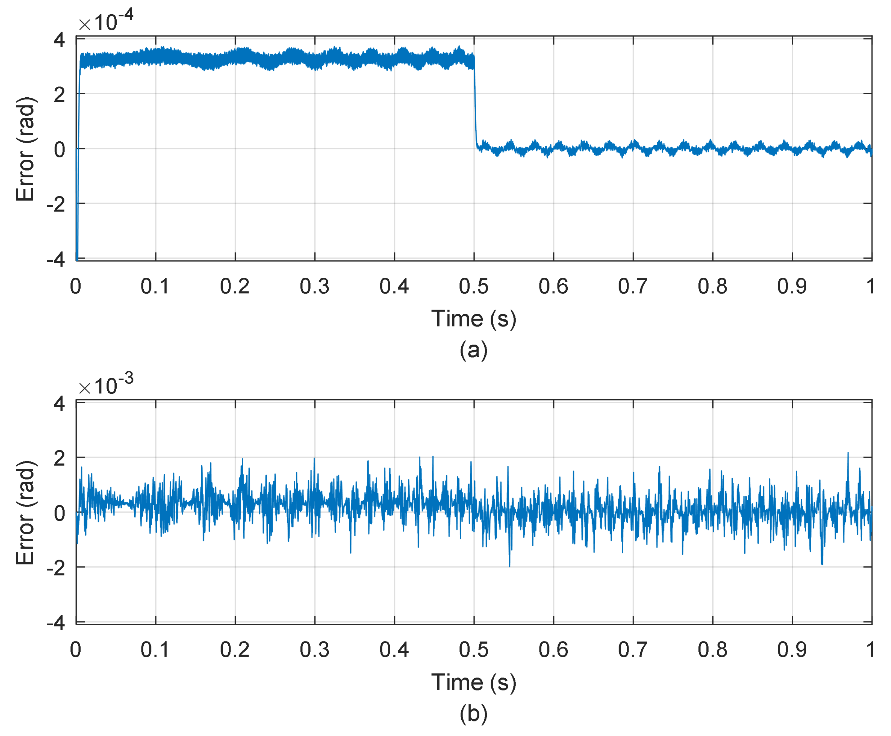
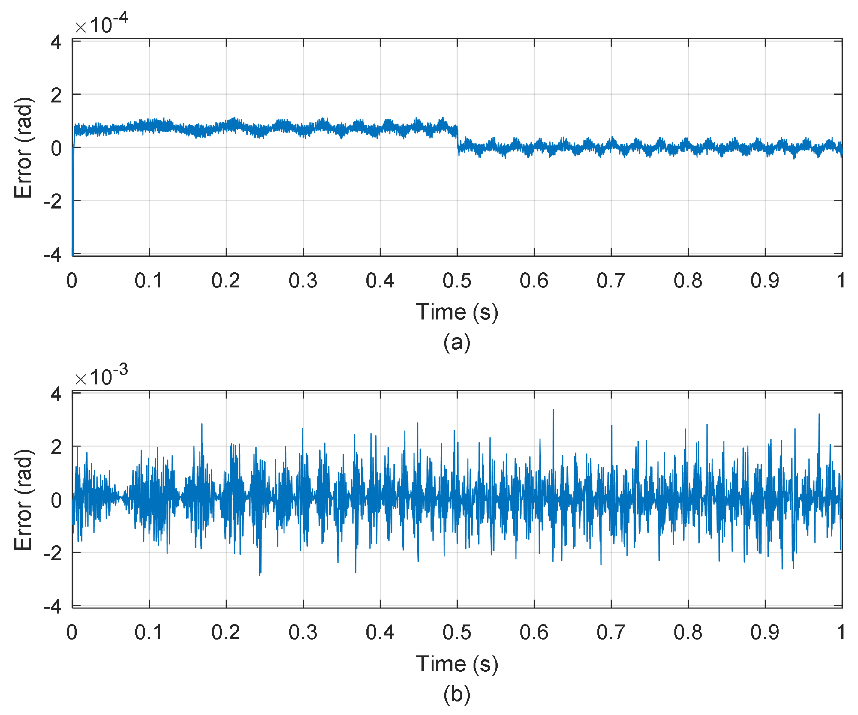
4.2. Experimental Results

An experimental platform based on hardware-in-the-loop (HIL) was set up to test the proposed ATO. The experimental setup shown in Figure 14 consists of a PC and the FPGA Development and Education Board DE2-115 of ALTERA (based on the FPGA EP4CE115F29C7). An Ethernet cable allowed communication between the FPGA board and the PC.

In this paper’s HIL testing method, the resolver signals were generated through a Simulink block diagram in the PC. These signals were sent to the FPGA board through the Ethernet cable. The FPGA board received these signals, estimated the angular position through the proposed ATO algorithm, and sent this estimation to the PC block diagram to calculate the angle estimation error. One main advantage of using the HIL method is that the angular position is known in each instant. Thus, the angle estimation error can be calculated with accuracy without requiring high-precision sensors (e.g., 16 bit absolute encoders, which are expensive). Furthermore, different from the simulations, HIL tests allow evaluating the actual effects of implementation problems (e.g., processing delays and the number of bits used in arithmetic operations) in the execution of an algorithm (the ATO in this case) in a digital processor. On the other hand, when a practical resolver is used, an additional angular position sensor with better accuracy (which is difficult to obtain) is required to get the actual angular position.

The proposed ATO was implemented in the FPGA board through a VHDL code, considering the same signal sampling frequency (50 kHz) and the SOD-GPC parameters used in the simulation tests. It was used as a fixed-point data format to perform the arithmetic operations with 32 bits. However, the estimated angular position was represented using 40 bits (30 fractional bits) to better compare the actual and the estimated angle. The emulated resolver signals were the same as those used in the simulation tests.

It was not possible to properly implement the ATO in Figure 7 in the FPGA using 32 bit fixed-point number representation. The main problem was the discretization of the integrators considering a sampling rate of 50 kHz. On the other hand, the SOD-GPC is a discrete-time control system, it being easier to implement in a digital processor (no discretization is needed). As a result, the proposed RDC based on a SOD-GPC-based ATO had a fast response, robustness against noise, and is suitable to implement in digital processors such as FPGAs. However, the PI-based ATO shown in Figure 8, whose structure is simple, was implemented in the FPGA. The same PI regulator used in the simulations, $C\left(z\right)=\frac{500.52(z-0.957)}{z-1}$, was applied in the experimental tests. As in the simulations, each integrator whose output is the estimated angle was implemented in the FPGA through forward Euler approximation, while backward Euler approximation was used to implement the other integrators.

Figure 15, Figure 16, Figure 17 and Figure 18 show the results for the HIL tests. In the tests without noise, it is possible to see a ripple in the angular position error during constant speed operation (from 0 s to 1 s). This ripple is produced by the limited number of bits used for the arithmetic operations. However, that ripple is negligible (that ripple has an amplitude less than $5\times {10}^{-5}$ rad).

Table 4. RMSE and settling time in the experimental HIL tests.

Configuration	RMSE (without Noise)	RMSE (with Noise)	Settling Time (s)
$N_p=102,N_c=2,{\overline{R}}_w=0.01$	$0.18\times {10}^{-3}$	$0.48\times {10}^{-3}$	$5.50\times {10}^{-3}$
$N_p=120,N_c=2,{\overline{R}}_w=0.01$	$0.23\times {10}^{-3}$	$0.47\times {10}^{-3}$	$5.90\times {10}^{-3}$
$N_p=102,N_c=10,{\overline{R}}_w=0.01$	$0.06\times {10}^{-3}$	$0.69\times {10}^{-3}$	$3.90\times {10}^{-3}$
PI-based ATO	$0.14\times {10}^{-3}$	$0.47\times {10}^{-3}$	$11.8\times {10}^{-3}$

presents the RMSE and the settling time obtained in each HIL test. These values are similar to those obtained in the simulations. If the value of $N_c$ rises, the ATO system will respond faster, but the RMSE will consequently be greater as well. Although the estimation error using the PI had a low RMSE, in the same order as the results obtained, the settling time for the PI-based ATO was almost twice the value obtained for the proposed approach. Besides, the PI-based ATO generated an overshoot ($2.8621\times {10}^{-4}$ rad) and an undershoot ($9.4647\times {10}^{-5}$ rad), which did not occur in the proposed ATO.

5. Conclusions

This paper presents a new angle tracking observer (ATO) based on a second-order difference GPC system (SOD-GPC). The proposed ATO has a steady-state error that tends to zero during constant speed operation, being faster and more robust than other ATOs. Besides, the estimated angular speed can be obtained by filtering the signal u(k) generated by the SOD-GPC algorithm (the design of that filter is beyond the objectives of this research). The GPC approach applied in this work is a discrete-time control system. Hence, the GPC structure is suitable for implementation in a digital processor. Other ATOs, as in [56], are based on the discretization of continuous-time tracking systems. The discretization may reduce the performance of a control system. The proposed ATO’s dynamic behavior depends on the values of $N_p$, $N_c$, and ${\overline{R}}_w$. Besides, the proposed ATO has a faster response than the PI-based ATO. In future works, heuristic techniques such as genetic algorithms will be used for ATO tuning. Furthermore, experimental tests using a physical resolver and a reference angular position sensor (e.g., a 16 bit absolute encoder) will be performed. However, the tests done in this research indicate that the application of the SOD-GPC algorithm to reduce the angle estimation error allows having a better estimation than using other types of closed-loop regulators (e.g., PI regulators).

References

1. Datlinger, C.; Hirz, M. An Extended Approach for Validation and Optimization of Position Sensor Signal Processing in Electric Drive Trains. Electronics 2019, 8, 77. [Google Scholar] [CrossRef] [Green Version]
2. Luo, P.; Tang, Q.; Jing, H.; Chen, X. Design and development of a self-calibration-based inductive absolute angular position sensor. IEEE Sens. J. 2019, 19, 135–142. [Google Scholar] [CrossRef]
3. Jeon, N.; Lee, H. Integrated fault diagnosis algorithm for motor sensors of in-wheel independent drive electric vehicles. Sensors 2016, 16, 2106. [Google Scholar] [CrossRef] [Green Version]
4. Mok, H.S.; Kim, S.H.; Cho, Y.H. Reduction of PMSM torque ripple caused by resolver position error. Electron. Lett. 2007, 43, 646–647. [Google Scholar] [CrossRef]
5. Kovacs, I.; Iosub, A.; Ţopa, M.; Buzo, A.; Pelz, G. On the influence of angle sensor nonidealities on the torque ripple in PMSM systems—An analytical approach. In Proceedings of the 2016 13th International Conference on Synthesis, Modeling, Analysis and Simulation Methods and Applications to Circuit Design (SMACD), Lisbon, Portugal, 27–30 June 2016. [Google Scholar]
6. Hwang, M.-H.; Lee, H.-S.; Cha, H.-R. Analysis of Torque Ripple and Cogging Torque Reduction in Electric Vehicle Traction Platform Applying Rotor Notched Design. Energies 2018, 11, 3053. [Google Scholar] [CrossRef] [Green Version]
7. Liu, Y.; Fang, J.; Tan, K.; Huang, B.; He, W. Sliding Mode Observer with Adaptive Parameter Estimation for Sensorless Control of IPMSM. Energies 2020, 13, 5991. [Google Scholar] [CrossRef]
8. Wachowiak, D. Genetic Algorithm Approach for Gains Selection of Induction Machine Extended Speed Observer. Energies 2020, 13, 4632. [Google Scholar] [CrossRef]
9. Liu, T.-H.; Ahmad, S.; Mubarok, M.S.; Chen, J.-Y. Simulation and Implementation of Predictive Speed Controller and Position Observer for Sensorless Synchronous Reluctance Motors. Energies 2020, 13, 2712. [Google Scholar] [CrossRef]
10. Woldegiorgis, A.T.; Ge, X.; Li, S.; Hassa, M. Extended sliding mode disturbance observer-based sensorless control of IPMSM for medium and high-speed range considering railway application. IEEE Access 2019, 7, 175302–175312. [Google Scholar] [CrossRef]
11. Chen, S.; Zhao, Y.; Qiu, H.; Ren, X. High-precision rotor position correction strategy for high-speed permanent magnet synchronous motor based on resolver. IEEE Trans. Power Electron. 2020, 35, 9716–9726. [Google Scholar] [CrossRef]
12. Datlinger, C.; Hirz, M. Benchmark of Rotor Position Sensor Technologies for Application in Automotive Electric Drive Trains. Electronics 2020, 9, 1063. [Google Scholar] [CrossRef]
13. Saneie, H.; Nasiri-Gheidari, Z.; Tootoonchian, F. Accuracy improvement in variable reluctance resolvers. IEEE Energy Convers. 2019, 34, 1563–1571. [Google Scholar] [CrossRef]
14. Hou, B.; Zhou, B.; Song, M.; Lin, Z.; Zhang, R. A Novel Single-Excitation Capacitive Angular Position Sensor Design. Sensors 2020, 16, 1196. [Google Scholar] [CrossRef]
15. Tang, T.; Chen, S.; Huang, X.; Yang, T.; Qi, B. Combining load and motor encoders to compensate nonlinear disturbances for high precision tracking control of gear-driven gimbal. Sensors 2018, 18, 754. [Google Scholar] [CrossRef] [Green Version]
16. Ni, Q.; Yang, M.; Odhano, S.A.; Tang, M.; Zanchetta, P.; Liu, X.; Xu, D. A new position and speed estimation scheme for position control of PMSM drives using low-resolution position sensors. IEEE Trans. Ind. Appl. 2019, 55, 3747–3758. [Google Scholar] [CrossRef] [Green Version]
17. Xiao, L.; Li, Z.; Bi, C. An optimization approach to variable reluctance resolver. IEEE Trans. Magn. 2020, 56, 7509005. [Google Scholar] [CrossRef]
18. Hajmohammadi, S.; Alipour-Sarabi, R.; Nasiri-Gheidari, Z.; Tootoonchian, F. Influence of different installation configurations on the position error of a multiturn wound-rotor resolver. IEEE Sens. J. 2020, 20, 5785–5792. [Google Scholar] [CrossRef]
19. Sun, L.; Taylor, J.; Dorneles Callegaro, A.; Emadi, A. Stator-pm-based variable reluctance resolver with advantage of motional back-emf. IEEE Trans. Ind. Electron. 2020, 67, 9790–9801. [Google Scholar] [CrossRef]
20. Bahari, M.; Davoodi, A.; Saneie, H.; Tootoonchian, F.; Nasiri-Gheidari, Z. A new variable reluctance pm-resolver. IEEE Sens. J. 2020, 1, 125–142. [Google Scholar] [CrossRef]
21. Wang, K.; Wu, Z. Hardware-based synchronous envelope detection strategy for resolver supplied with external excitation generator. IEEE Access 2019, 7, 20801–20810. [Google Scholar] [CrossRef]
22. Wang, S.; Kang, J.; Degano, M.; Buticchi, G. A resolver-to-digital conversion method based on third-order rational fraction polynomial approximation for PMSM control. IEEE Trans. Ind. Electron. 2019, 66, 6383–6392. [Google Scholar] [CrossRef]
23. Bennamar, M.; Gonzales, A.S.P. A Novel PLL resolver angle position indicator. IEEE Trans. Instrum. Meas. 2016, 65, 123–131. [Google Scholar] [CrossRef]
24. Staebler, M.; Verma, A. TMS320F240 DSP Solution for Obtaining Resolver Angular Position and Speed; Texas Instrument Inc.: Dallas, TX, USA, 2017. [Google Scholar]
25. Abou Qamar, N.; Hatziadoniu, C.J.; Wang, H. Speed error mitigation for a DSP-based resolver-to-digital converter using autotuning filters. IEEE Trans. Ind. Electron. 2015, 62, 1134–1139. [Google Scholar] [CrossRef] [Green Version]
26. Kaewjinda, W.; Konghirun, M.A. DSP—based vector control of pmsm servo drive using resolver sensor. In Proceedings of the 2006 IEEE Region 10 Conference (TENCON), Hong Kong, China, 14–17 November 2006; pp. 1–4. [Google Scholar]
27. Idkhajine, L.; Monmasson, E.; Naouar, M.W.; Prata, A.; Boullaga, K. Fully integrated FPGA-based controller for synchronous motor drive. IEEE Trans. Ind. Electron. 2009, 56, 4006–4017. [Google Scholar] [CrossRef]
28. Garcia, R.C.; Pinto, J.O.P.; Suemitsu, W.I.; Soares, J.O. Improved demultiplexing algorithm for hardware simplification of sensored vector control through frequency-domain multiplexing. IEEE Trans. Ind. Electron. 2017, 64, 6538–6548. [Google Scholar] [CrossRef]
29. Smidl, V.; Janous, S.; Peroutka, Z.; Adam, L. Time-optimal current trajectory for predictive speed control of PMSM drive. In Proceedings of the 2017 IEEE International Symposium on Predictive Control of Electrical Drives and Power Electronics (PRECEDE), Pilsen, Czech Republic, 4–6 September 2017; pp. 83–88. [Google Scholar]
30. Moreno, J.C.; Espi Huerta, J.M.; Gil, R.G.; Gonzalez, S.A. A robust predictive current control for three-phase grid-connected inverters. IEEE Trans. Ind. Electron. 2009, 56, 1993–2004. [Google Scholar] [CrossRef]
31. Camacho, E.F.; Bordons, C. Model Predictive Control, 2nd ed.; Springer: London, UK, 2004; pp. 13–124. [Google Scholar]
32. Wang, L. Model Predictive Control System Design and Implementation Using Matlab®; Springer: London, UK, 2009; pp. 1–20. [Google Scholar]
33. Ruchika, N.R. Model predictive control: History and development. Int. J. Eng. Trends Technol. 2013, 4, 2600–2602. [Google Scholar]
34. Qin, S.J.; Badgwell, T.A. A survey of industrial model predictive control technology. In Proceedings of the 2016 European Control Conference (ECC), Aalborg, Denmark, 29 June–1 July 2016; pp. 733–764. [Google Scholar]
35. Clarke, D.W.; Mohtadi, C.; Tuffs, P.S. Generalized predictive control—Part I. the basic algorithm. Automatica 1987, 23, 137–148. [Google Scholar] [CrossRef]
36. Clarke, D.W.; Mohtadi, C.; Tuffs, P.S. Generalized Predictive Control—Part II. Extensions and Interpretations. Automatica 1987, 23, 149–160. [Google Scholar] [CrossRef]
37. Prajwowski, K.; Golebiewski, W.; Lisowski, M.; Abramek, K.F.; Galdynski, D. Modeling of working machines synergy in the process of the hybrid electric vehicle acceleration. Energies 2020, 13, 5818. [Google Scholar] [CrossRef]
38. Wang, F.; Zhang, Z.; Mei, X.; Rodríguez, J.; Kennel, R. Advanced control strategies of induction machine: Field oriented control, direct torque control and model predictive control. Energies 2018, 11, 120. [Google Scholar] [CrossRef] [Green Version]
39. Gonçalves, P.; Cruz, S.; Mendes, A. Finite control set model predictive control of six-phase asymmetrical machines—An overview. Energies 2019, 12, 4693. [Google Scholar] [CrossRef] [Green Version]
40. Nguyen, T.-T.; Yoo, H.-J.; Kim, H.-M.; Nguyen-Duc, H. Direct phase angle and voltage amplitude model predictive control of a power converter for microgrid applications. Energies 2018, 11, 2254. [Google Scholar] [CrossRef] [Green Version]
41. Jin, N.; Pan, C.; Li, Y.; Hu, S.; Fang, J. Model predictive control for virtual synchronous generator with improved vector selection and reconstructed current. Energies 2020, 13, 5435. [Google Scholar] [CrossRef]
42. Abdelrahem, M.; Hackl, C.M.; Rodríguez, J.; Kennel, R. Model reference adaptive system with finite-set for encoderless control of PMSGs in micro-grid systems. Energies 2020, 13, 4844. [Google Scholar] [CrossRef]
43. Turley, C.; Jacoby, M.; Pavlak, G.; Henze, G. Development and evaluation of occupancy-aware hvac control for residential building energy efficiency and occupant comfort. Energies 2020, 13, 5396. [Google Scholar] [CrossRef]
44. Bahramnia, P.; Hosseini Rostami, S.M.; Wang, J.; Kim, G.-J. Modeling and controlling of temperature and humidity in building heating, ventilating, and air conditioning system using model predictive control. Energies 2019, 12, 4805. [Google Scholar] [CrossRef] [Green Version]
45. Estrabis, T.; Cordero, R.; Batista, E.; Andrea, C.; Grassi, M.A.S. Application of model predictive control in a resolver-to-digital converter. In Proceedings of the 2019 IEEE 15th Brazilian Power Electronics Conference and 5th IEEE Southern Power Electronics Conference (COBEP/SPEC), Santos, Brazil, 1–4 December 2019; pp. 1–6. [Google Scholar]
46. Dorf, R.C.; Bishop, R.H. Modern Control Systems, 8th ed.; Addison Wesley Longman, Inc.: Menlo Park, CA, USA, 1998; pp. 662–666. [Google Scholar]
47. Belda, K.; Vosmik, D. Explicit generalized predictive control of speed and position of PMSM drives. IEEE Trans. Ind. Electron. 2016, 63, 3889–3896. [Google Scholar] [CrossRef]
48. Maeder, U.; Morari, M. Offset-free reference tracking with model predictive control. Automatica 2010, 46, 1469–1476. [Google Scholar] [CrossRef]
49. Cordero, R.; Estrabis, T.; Batista, E.A.; Andrea, C.Q.; Gentil, G. Ramp-tracking generalized predictive control system based on second-order difference. IEEE Trans. Circuits Syst. II Exp. Briefs 2020. to be published. [Google Scholar] [CrossRef]
50. Jerry, A.J. Difference Equations with Discrete Transform Methods; Springer Science+Business Media: Dordrecht, The Netherlands, 1996; pp. 1–22. [Google Scholar]
51. Proakis, J.C.; Manolakis, D.G. Digital Signal Processing: Principles, Algorithms and Applications, 3rd ed.; Prentice-Hall, Inc.: Upper Saddle River, NJ, USA, 1996. [Google Scholar]
52. Wu, Z.; Li, Y. High-accuracy automatic calibration of resolver signals via two-step gradient estimators. IEEE Sens. J. 2018, 18, 2883–2891. [Google Scholar] [CrossRef]
53. Sarma, S.; Venkateswaralu, A. Systematic error cancellations and fault detection of resolver angular sensors using a DSP based system. Mechatronics 2009, 19, 1303–1312. [Google Scholar] [CrossRef]
54. Noori, N.; Khaburi, D.A. Diagnosis and compensation of amplitude imbalance, imperfect quadrant and offset in resolver signals. In Proceedings of the 2016 7th Power Electronics and Drive Systems Technologies Conference (PEDSTC), Tehran, Iran, 16–18 February 2016; pp. 76–81. [Google Scholar]
55. Gao, Z.; Zhou, B.; Hou, B.; Li, C.; Wei, Q.; Zhang, R. Self-calibration of nonlinear signal model for angular position sensors by model-based automatic search algorithm. Sensors 2019, 19, 2760. [Google Scholar] [CrossRef] [Green Version]
56. Cordero, R.; Pinto, J.O.P.; Ono, I.E.; Fahed, H.D.S.; Brito, M. Simplification of the acquisition system for sensored vector control using resolver sensor based on fdm and current synchronous sampling. In Proceedings of the 2018 IEEE 4th Southern Power Electronics Conference (SPEC), Singapore, 10–13 December 2018; pp. 1–4. [Google Scholar]
Figure 1. Schematic diagram of the resolver sensor.
Energies 14 00459 g001
Figure 2. Conventional generalized predictive control described in [32].
Energies 14 00459 g002
Figure 3. Schematic of the second-order difference GPC system (SOD-GPC).
Energies 14 00459 g003
Figure 4. Proposed ATO based on the SOD-GPC.
Energies 14 00459 g004
Figure 5. Simplified block diagram of the proposed ATO considering only the effect of e θ ( k ) in the angle estimation.
Energies 14 00459 g005
Figure 6. Speed curve used in the tests.
Energies 14 00459 g006
Figure 7. RDC system described in [56].
Energies 14 00459 g007
Figure 8. PI-based ATO.
Energies 14 00459 g008
Figure 9. Simulation results for N p = 102 , N c = 2 , R ¯ w = 0.01 . (a) Without noise; (b) with noise.
Energies 14 00459 g009
Figure 10. Simulation results for N p = 120 , N c = 2 , R ¯ w = 0.01 . (a) Without noise; (b) with noise.
Energies 14 00459 g010
Figure 11. Simulation results for N p = 102 , N c = 10 , R ¯ w = 0.01 . (a) Without noise; (b) with noise.
Energies 14 00459 g011
Figure 12. Simulation results for the ATO in [56]. (a) Without noise; (b) with noise.
Energies 14 00459 g012
Figure 13. Simulation results for the PI-based ATO. (a) Without noise; (b) with noise.
Energies 14 00459 g013
Figure 14. Experimental setup.
Energies 14 00459 g014
Figure 15. Experimental results for N p = 102 , N c = 2 , R ¯ w = 0.01 . (a) Without noise; (b) with noise.
Energies 14 00459 g015
Figure 16. Experimental results for N p = 120 , N c = 2 , R ¯ w = 0.01 . (a) Without noise; (b) with noise.
Energies 14 00459 g016
Figure 17. Experimental results for N p = 102 , N c = 10 , R ¯ w = 0.01 . (a) Without noise; (b) with noise.
Energies 14 00459 g017
Figure 18. Experimental results for the PI-based ATO. (a) Without noise; (b) with noise.
Energies 14 00459 g018