Article

Real-Gas-Flamelet-Model-Based Numerical Simulation and Combustion Instability Analysis of a GH2/LOX Rocket Combustor with Multiple Injectors

1
Department of Aerospace Engineering, Pusan National University, Pusan 46241, Korea
2
Department of Mechanical Engineering, Pohang University of Science and Technology, Pohang 37673, Korea
3
Institute of Advanced Aerospace Technology, Seoul National University, Seoul 08826, Korea
4
Department of Mechanical Engineering, Sejong University, Seoul 05006, Korea
*
Author to whom correspondence should be addressed.
Energies 2021, 14(2), 419; https://doi.org/10.3390/en14020419
Submission received: 10 December 2020 / Revised: 5 January 2021 / Accepted: 9 January 2021 / Published: 13 January 2021
(This article belongs to the Special Issue Propulsion and Combustion in Aerospace Systems)

Abstract

:
A large eddy simulation (LES) and combustion instability analysis are performed using OpenFOAM for the multiple shear-coaxial injector combustor DLR-BKD (in German Deutsches Zentrum für Luft–Brennkammer D, German Aerospace Center–Combustion Chamber D), which is a laboratory-scale combustor operating in a real-gas environment. The Redlich–Kwong–Peng–Robinson equation of state and steady-laminar flamelet model are adopted in the simulation to accurately capture the real-gas combustion effects. Moreover, the stable combustion under the LP4 condition is numerically analyzed, and the characteristics of the combustion flow field are investigated. In the numerical simulation of the combustion instability, the instability is generated by artificially superimposing the 1st transverse standing wave solution on the stable combustion solution. To decompose the combustion instability mode, the dynamic mode decomposition method is applied. Several combustion instability modes are qualitatively and quantitatively identified through contour plots and graphs, and the sustenance process of the limit cycle is investigated.

1. Introduction

When combustion instability occurs, the vibration generated during the combustion, disturbances in the propellant supply system, and acoustic fields affect the pressure, temperature, and flow rate in the combustion chamber, leading to the persistence of the unstable state. This instability is characterized by large pressure fluctuations at a specific frequency or excessive heat transfer. In particular, the high-frequency combustion instability is caused by the interference between the combustion chamber and sound waves inside the combustion chamber, generally corresponding to the frequency range of 1 kHz or higher [1]. In the case of high-frequency combustion instability, the energy perturbation emitted during the combustion process is combined with a specific acoustic mode in the combustion chamber, which rapidly amplifies the pressure fluctuation. This high-frequency combustion instability may be highly destructive, and in the absence of proper control devices such as baffles, acoustic liners, and acoustic cavities, the chamber may be destroyed or undergo melting.
Recently, several experiments were conducted to examine the high-frequency combustion instability in a real-gas condition for lab-scale combustors employing a single injector [2,3] and multiple injectors [4,5,6]. Moreover, many researchers performed numerical analyses for liquid rocket combustors. The flame structure and temperature distribution inside the combustor were analyzed using various simulation tools, combustion models, and RANS models. However, these analyses could not capture the actual structure and dynamics of 3D turbulent flame owing to the use of RANS models [7,8,9,10,11]. Furthermore, LES studies on a liquid rocket combustor were performed [12,13,14]. The combustion instability was investigated by conducting numerical analyses, and several authors used the LES technique to extensively analyze the combustion instability mode generated in liquid rocket combustors or gas turbine engines [15,16,17,18].
Schulze et al. [19] performed a numerical analysis for the shear-coaxial injector combustor DLR-BKD, using hydrogen and oxygen as propellants. Specifically, the authors performed an axisymmetric simulation on a single injector among multiple injectors of the combustor. The periodic velocity fluctuation condition was assigned as the boundary condition to artificially create and analyze the combustion instability. Various fields such as those of the temperature, density, mass fraction, and heat release rate were visualized, and the fluctuating fields were decomposed through the dynamic mode decomposition (DMD) technique to investigate the modes of the fluctuating fields.
In addition, Urbano et al. [20] performed a numerical analysis for the DLR-BKD combustor. The complete geometry of the combustor, including the multiple injectors and manifolds supplying the propellants, was considered. An LES was performed using the 4th and 3rd order accuracies in time and space, respectively, and the fast chemistry model was used as a combustion model. The Soave–Redlich–Kwong (SRK) model was adopted as the real-gas equation model. Instead of the flow and flame structure, the authors analyzed the eigen-frequency and eigen-modes that caused combustion instability.
Furthermore, Urbano et al. [21] adopted the same numerical analysis methods as in the previous study [20] and performed the numerical analysis for the DLR-BKD combustor considering a single injector rather than all the injectors. The correlation among the unsteady heat release rate, pressure fluctuation, and velocity fluctuation of the injection jet for a single injector was analyzed using graphs, based on which, the underlying mechanism of the combustion instability was examined. Moreover, the authors attempted to derive the gain and time delay values related to the time lag model.
Schmitt et al. [22] performed a numerical analysis for the BKD combustor using the same methods as those adopted by Urbano et al. [20]. The authors focused on the visualization of the temperature, velocity, and density fields. In addition, the combustion instability was generated to investigate the pressure oscillation in the combustor. However, the analysis was not extensive and limited to the overall flow characteristics of the combustor.
In this study, an LES and combustion instability analysis for the BKD combustor, which is a lab-scale combustor operating in a real-gas condition, are conducted using the open source CFD software OpenFOAM with a reacting flow solver developed to realize the simulation of high-pressure liquid rocket combustors. To accurately capture the real-gas combustion effect, the Redlich–Kwong–Peng–Robinson (RK–PR) state equation and steady-laminar flamelet model (SLFM) are adopted. To induce the combustion instability mode, the DMD method is employed, and the combustion instability according to the mode is qualitatively and quantitatively identified through contour plots and graphs. Moreover, the sustenance process of the combustion instability is evaluated.

2. DLR-BKD Combustor

The DLR-BKD combustor operating on the p8 test bench at the German Aerospace Center (DLR)’s Lampoldshausen site is a lab-scale liquid rocket engine consisting of 42 shear-coaxial injectors [4]. The p8 test bench is designed to study the high-pressure H2/LOx combustion in liquid rocket engines, and the facility can supply H2 and LOx with mass flow rates of 1.5 kg/s and 8 kg/s, respectively, under cryogenic conditions. As shown in Figure 1, the engine is composed of propellant manifolds, injectors, a combustion chamber, and an exhaust nozzle. A measurement ring equipped with eight dynamic pressure sensors to measure the dynamic pressure inside the chamber is located between the injector face plate and combustion chamber. Oxygen is supplied to the oxygen manifold in a compressible liquid state and injected at the injector in a supercritical state. Hydrogen is introduced into the hydrogen manifold in a supercritical state and injected at the injector in the same state. The injector is a shear-coaxial type, with the oxygen and hydrogen being injected from the center and annular orifices, respectively. The propellant supply conditions and theoretical combustion pressure and temperature are summarized in Table 1. The critical properties of oxygen and hydrogen are p c r , O 2 = 50.4 bar, T c r , O 2   = 155 K, and p c r , H 2 = 13 bar, T c r , H 2   = 33 K, respectively. The supply condition detailed in Table 1 is termed as LP4, and it represents the experimental condition accompanying the combustion instability for the combustor.

3. Numerical Setup

3.1. Governing Equations

Herein, the LES of turbulent combustion is performed to obtain the unsteady flow and flame fields. Therefore, two transport equations, i.e., the mixture fraction and mixture fraction variance equations are solved in addition to the continuity and Navier–Stokes equations. All the equations are solved considering a three-dimensional system, and Favre filtering ( ϕ ˜ = ρ ϕ ¯ / ρ ¯ ) is applied to resolve the large-scale eddies. The filtered equations can be expressed as Equations (1)–(4).
ρ ¯ t + ρ ¯ u ˜ i x i = 0
ρ ¯ u ˜ i t + ρ ¯ u ˜ i u ˜ j x j = p ¯ x j + τ ¯ i j x j τ i j s g s x j
ρ ¯ z ˜ t + ρ ¯ u ˜ j z ˜ x j = x j ( μ t S c t z ˜ x j )
ρ ¯ z 2 ˜ t + ρ ¯ u ˜ j z 2 ˜ x j = x j ( μ t S c t z 2 ˜ x j ) + 2 μ t S c t ( z ˜ x j ) 2 ρ ¯ χ ˜
The variables ρ , u , t , and x in Equation (1) denote the fluid density, velocity, time, and coordinate component, respectively. p , τ , and τ s g s in Equation (2) denote the pressure, viscous stress, and sub-grid scale stress, respectively. z , μ t , and S c t in Equation (3) denote the mixture fraction, turbulent viscosity, and turbulent Schmidt number, respectively. The mixture fraction indicates the mass fraction of one stream of a mixture formed by two feed streams. z 2 and χ in Equation (4) denote the mixture fraction variance and scalar dissipation rate (SDR), respectively. The mixture fraction variance is defined as the average of the squared differences from the mean mixture fraction, and this value is related to the turbulence–chemistry interaction. The SDR controls the mixing and represents the gradient of the mixture fraction, which is related to the strain. In Equations (3) and (4), S c t = 0.6, as a suitable value to perform the combustion simulation of a GH2/LOx combustor in a real-gas condition [14].

3.2. Sub-Grid Scale Model

The sub-grid scale stress tensor τ i j s g s , which is related to the unresolved small-scale eddies, as indicated in Equation (2), is modeled. The Smagorinsky turbulence model [23] is based on Boussinesq’s eddy viscosity hypothesis, and the model expresses τ i j s g s as in Equation (5). The SGS viscosity μ s g s in Equation (5) is expressed as a function of the product of Δ and k s g s , as in Equation (6), selected to simulate the SGS eddy length and velocity, respectively. In the present study, the constant C k = 0.094 [24] is selected as an appropriate value for a wide range of flows. k s g s in Equation (6) can be expressed as in Equation (7) assuming that the generation and dissipation of the SGS eddy energy are in equilibrium, corresponding to the occurrence of the local equilibrium. The three coefficients in Equation (7) are expressed as A = C ϵ / Δ , B = 2 3 t r ( S ˜ i j ) , and C = 2 C k Δ [ S ˜ i j 1 3 t r ( S ˜ i j ) δ i j ] S ˜ i j , and the constant C ϵ = 1.048.
τ i j s g s = 2 μ s g s S ˜ i j + 2 3 k s g s δ i j
μ s g s = ρ C k Δ k s g s
k s g s = ( B + B 2 + 4 A C 2 A ) 2
The eddy viscosity in the Smagorinsky model is nonzero at solid boundaries, which is in contrast to the fact that the eddy viscosity is zero in the absence of turbulence. An easy solution to this aspect is to introduce the van Driest-style damping function [25] in the length scale. If the van Driest model is applied to Δ near the wall, Δ can be expressed as in Equation (8).
Δ v D = min ( Δ , κ C Δ ) y ( 1 e y + / A + )
where κ is the von Kármán constant, with a value of 0.4187. The derived constants C Δ and A + are 0.158 and 26, respectively. The limit of y + is 0–500.

3.3. Equation of State (EOS)

The RK–PR equation was developed by Cismondi and Mollerup [26] to overcome the limitations of the existing two-parameter cubic EOS models such as the SRK [27] and PR [28] equations. Among the existing two-parameter cubic EOS models, the PR equation can enhance the vapor pressure prediction of low-hydrocarbon species; however, the prediction accuracy is lower than that achieved by the SRK for fuels with C1–C4 alkanes. Moreover, as the pressure increases to high values of approximately 100 MPa, several species cannot be accurately predicted in terms of the critical compressibility factor compared to those predicted using the SRK. Therefore, Cismondi and Mollerup proposed the following equation to accurately predict the vapor pressure by combining the advantages of the two EOS models.
p = R T v b a c ( 3 2 + T r ) n ( v + δ 1 b ) ( v + 1 δ 1 1 + δ 1 b )
n = ( 1.168 A 1 Z c e x p + A 0 ) ω 2 + ( 1.168 B 1 Z c e x p + B 0 ) ω + ( 1.168 C 1 Z c e x p + C 0 ) δ 1 = d 1 + d 2 ( d 3 1.168 Z c e x p ) d 4 + d 5 ( d 3 1.168 Z c e x p ) d 6
The detailed description for the coefficients d 1 d 6 , A 0 C 0 , and A 1 C 1 in Equation (10) can be found in the literature [26]. The term ( v + δ 1 b ) ( v + 1 δ 1 1 + δ 1 b ) in Equation (9) represents a combination of the PR and SRK. The parameter δ 1 is obtained from the curve fitting process, and the constant 1.168 in Equation (10) is adopted to estimate the lowest density error for many species ( N 2 , ethylene, propane, CO 2 , pentane, hexane, heptane, octane, NH 3 ). The term a c ( 3 2 + T r ) n in Equation (9) is obtained from the curve fitting process, and the parameter n is adopted to match the vapor pressure reported previously. Moreover, the coefficients A 0 C 0 and A 1 C 1 are obtained from curve fitting n and the acentric factor.

3.4. Combustion Model

The SLFM approach can help solve the flame brushes of a turbulent flame by assuming each flame brush to be an ensemble of tiny discrete one-dimensional laminar diffusion flames. After performing a one-dimensional opposed-flow laminar diffusion flame analysis, the distributions of the scalar properties such as the density, temperature, and species mass fraction according to the mixture fraction space are obtained, and the constructed flamelet lookup table can be employed in the simulation. In the case of a turbulent flow, the probability density function (pdf) can be used to calculate the mixture fraction, and especially in the case of an axisymmetric jet flow, the β-pdf function can be suitably adopted. The β-pdf function used in the present study can be expressed as in Equations (11) and (12) [29]. In this case, the turbulent scalar properties in a flow field can be obtained through numerical integration with the pdf, as expressed in Equation (13).
P ˜ ( z ) = z α 1 ( 1 z ) β 1 Γ ( α ) Γ ( β ) Γ ( α + β )
α = z ˜ γ ,   β = ( 1 z ˜ ) γ ,   γ = z ˜ ( 1 z ˜ ) z 2 ˜
ϕ ˜ = ϕ ( z , χ s t ) P ˜ ( z ) P ˜ ( χ s t ) d z d χ s t
In Equation (11), the shape of the probability function varies according to the two parameters α and β , and Γ is the gamma function. α and β can be expressed in terms of the mixture fraction and its variance, as in Equation (12). Moreover, the scalar property ϕ , which is the function of the mixture fraction and SDR, can be density-weighted averaged through numerical integration, as indicated in Equation (13). The SDR χ ˜ in Equation (4) is modeled as in Equation (14) [30].
χ ˜ = C χ μ + μ t ρ ¯ S c t ( z ˜ x j ) 2
where C χ = 2 .
The chemical reaction mechanism considered in the evaluation of the one-dimensional laminar diffusion flame is based on the work of Conaire et al. [31]. The mechanism contains 11 species and 19 reaction steps. In the present study, eight chemical species (H2, O2, H, O, H2O, OH, HO2, H2O2) excluding N2, Ar, and He, and 12 reaction steps are adopted. This reaction is validated under conditions with the initial temperature of 298–2700 K, pressure of 0.05–87 atm, and equivalence ratio of 0.2–6. This mechanism is considered to be applicable in a high-pressure combustion environment such as a real-gas environment.

3.5. DMD

The DMD [32,33] approach can be used to calculate the mode set and its frequency f as well as the damping coefficient ξ i for the time series fields V m   and   V m + 1 , as expressed in Equation (15). Moreover, this approach can be used to investigate the unsteady fluid flow phenomenon in fluid mechanics. Mathematically, a theoretical matrix A of the linear equation system for the time series fields can be determined as in Equation (16). In particular, the singular value decomposition technique is used to derive the eigenvalues λ i and eigenvectors E i D M D for matrix A , as expressed in Equation (17), and the eigenvalue and eigenvector are derived by decomposing the eigenvalue from a non-square matrix. From the eigenvalue, the frequency and damping coefficient can be calculated as in Equations (18) and (19), respectively, and the mode shape can be derived from the real part of the eigenvector.
V m = [ v 1 , , v m ] ,   V m + 1 = [ v 2 , , v m + 1 ]
V m + 1 = AV m
AE i D M D = λ i E i D M D
A r g ( λ i ) = 2 π f i N s t e p Δ t + 2 π T
ξ i = l n | λ i | N s t e p Δ t
where N s t e p is the number of steps between two snapshots, Δ t is the time step size, and T is period.

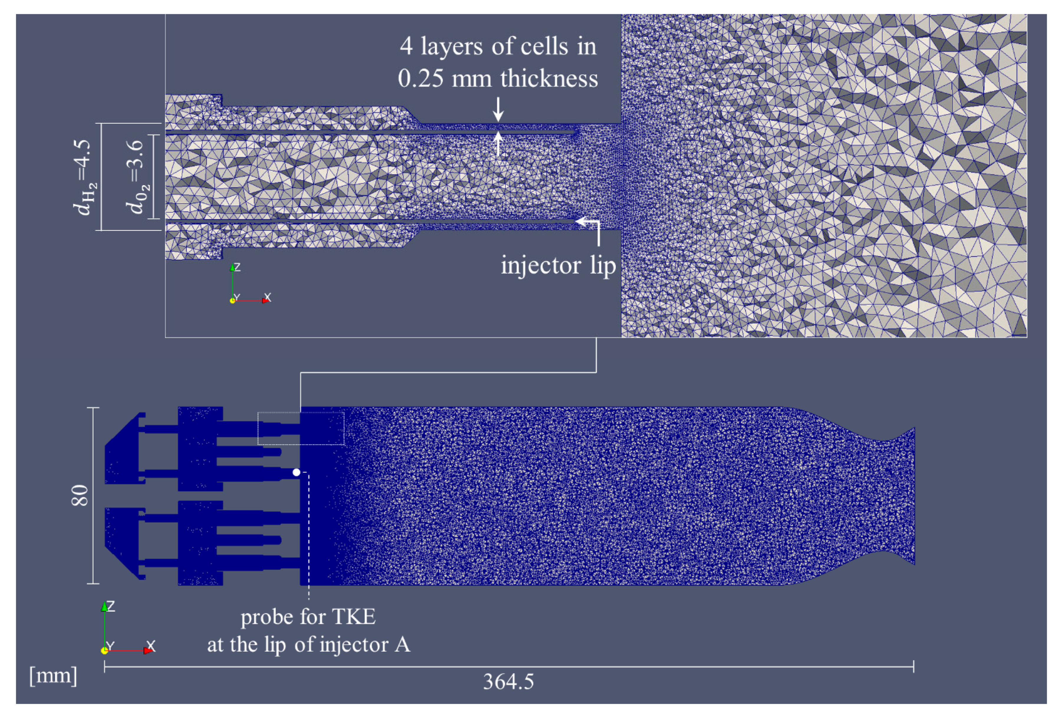
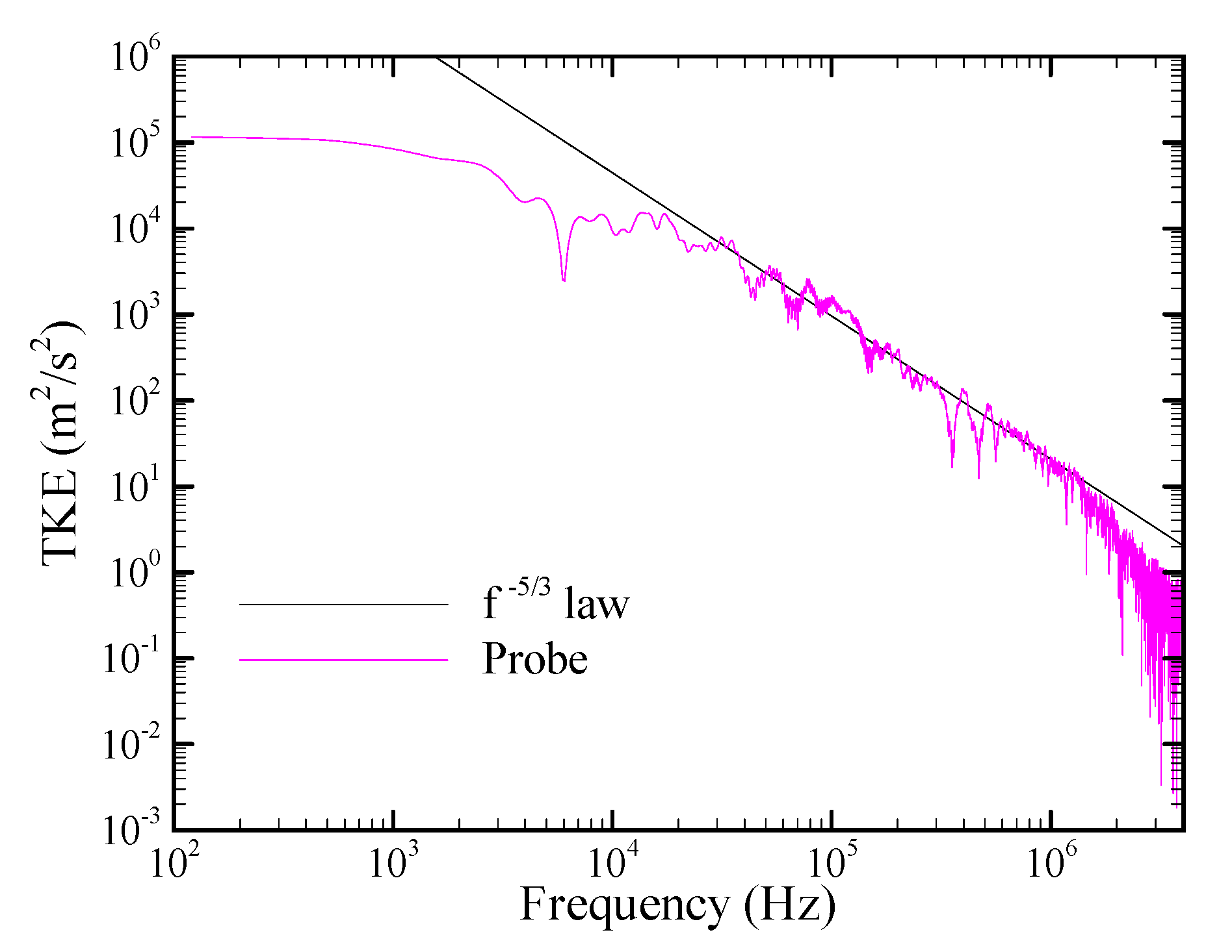
3.6. Computational Grid
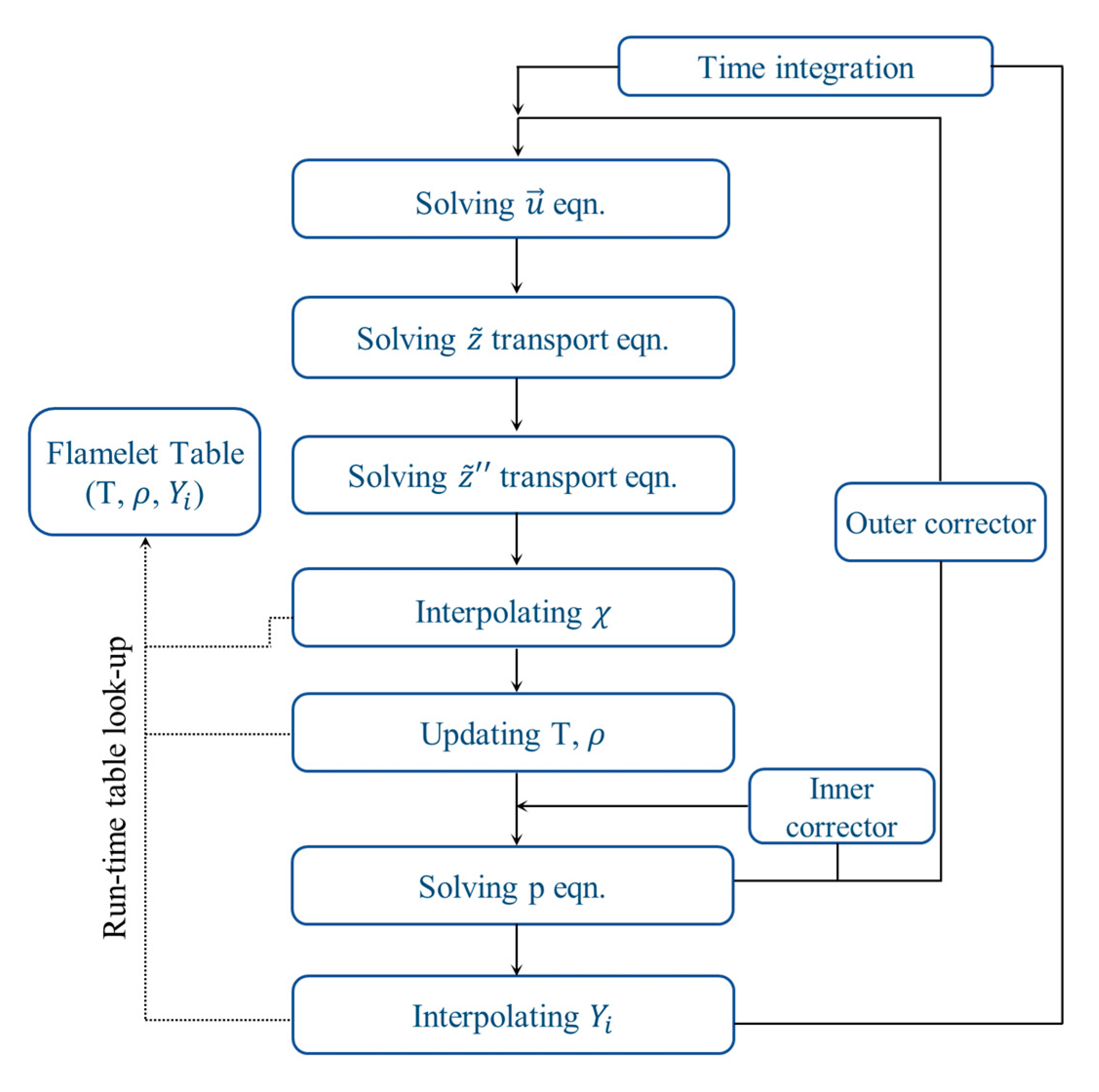
As shown in Figure 2, the grid system of the BKD combustor consists of tetrahedral cell elements because the geometry is slightly complex. The hydrogen injector has an annular pipe, with the minimum pipe width being 0.25 mm; consequently, the smallest cell is concentrated in that region and near the injector lip. To simulate parabolic flow in the annular pipe, at least four layers of cells are stacked in the radial direction. Moreover, the smallest cells are located near the injector lip to capture the vortex shedding occurring in the hydrogen–oxygen shear layer. The flow around the injector lip must be accurately simulated because the objective of this work is to confirm whether the limit cycle is maintained after the triggering of the combustion instability. In the simulations for a shear-coaxial injector combustor, the cell size near the injector lip ranges from at least the length of the lip thickness to a few fractions of the thickness to form and maintain the stable flame and observe the flame dynamics near the injector [14,22,34]. As reported previously, 500 million cells are required to realize a high-fidelity LES for the BKD combustor [20]; however, this value corresponds to an excessive computational burden. Therefore, in this study, the grid system is designed to have 70 million cells to minimize the computational requirement while maintaining the minimum criterion for the cells. As shown in Figure 2, a probe point is located next to the injector lip to measure the turbulent kinetic energy (TKE) throughout the simulation. As shown in Figure 3, the fast Fourier transform (FFT) of the TKE is examined to confirm Kolmogorov’s 5/3 law.

3.7. Solver Setup

In this study, the open source CFD software OpenFOAM is used as a simulation tool. Moreover, the reacting flow solver SLFMFoam_LES is developed and used for the present study. This solver combines the SLFM model and PIMPLE [35] algorithm, which is an unsteady flow algorithm, and the solver is developed to perform a LES of turbulent combustion. The PIMPLE algorithm combines the SIMPLE and PISO algorithms [36], which are steady- and unsteady-state flow algorithms, respectively. The detailed framework of the SLFMFoam_LES solver is illustrated in Figure 4. This solver solves the momentum, mixture fraction, and mixture fraction variance equations in order and calculates the SDR. Subsequently, the temperature, density, and species mass fraction for the SDR in the flamelet table are linearly interpolated. Next, because this solver is a segregated solver, the pressure equation is solved separately, and the outer correction is repeated according to the nature of the SIMPLE algorithm. When the calculation converges, the algorithm moves to the next time step.
For the temporal discretization, the implicit Euler scheme with first-order accuracy is used for all the equations. For the spatial discretization, the minmod limiter [37] with second-order accuracy is used for the convective terms of all the equations. In addition, the linear scheme with second-order accuracy is used for the diffusion terms of all the equations.
The boundary conditions are established as follows. A fixed mass flow rate condition is applied to both the hydrogen and oxygen inlets. The non-slip condition is applied to all the walls. The fixed pressure and extrapolation conditions are applied to the nozzle outlet. The van Driest model is applied to the walls for the boundary layer treatment.
The SDR range of the flamelet table is 105–50,000. Figure 5 shows the scalar properties according to the mixture fraction obtained from the flamelet table. Figure 5a shows the temperature graph. The stoichiometric mixture fraction value is located at z = 0.12, and the maximum temperature reaches 3627 K at this location. It is considered that the change in the scalar property according to the SDR difference is not significant. Figure 5b shows the density graph. Because the density change is particularly severe near z = 0–0.004, which is near the pure oxygen domain, the gradient change is reproduced in the smaller frame.
The total flow time is set as 16 ms, and the Courant–Friedrichs–Lewy number is set as 1 corresponding to the time step size of approximately 1 × 10⁻⁸ s. In terms of the computational resource, 1224 cores of Intel Xeon Gold 6154 3.0 GHz are used for the simulation, corresponding to 117.5 TFLOPS. The total wall clock time is 181 h/ms, corresponding to 122,000 CPU-h/ms.

4. Results and Discussion

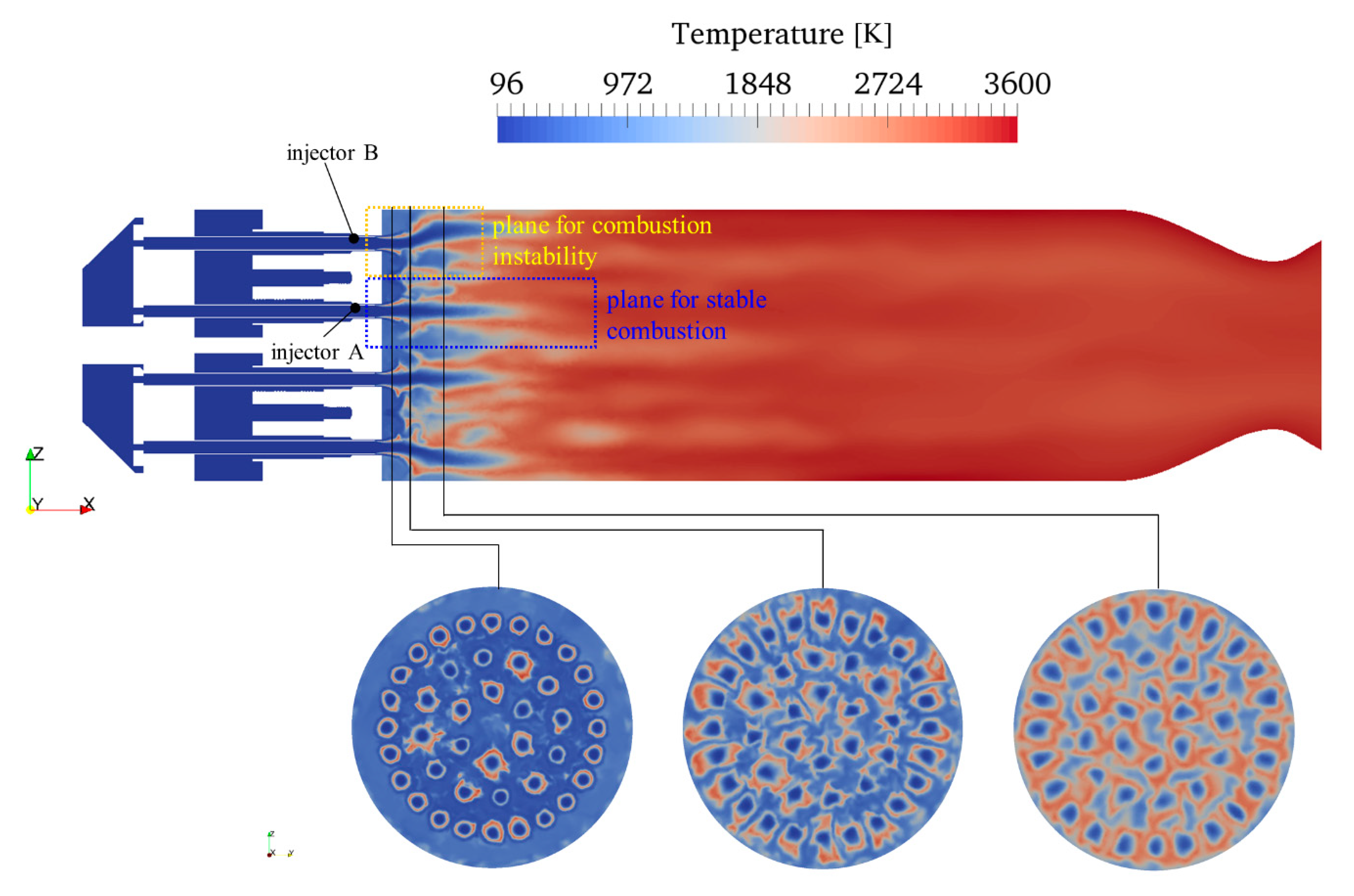
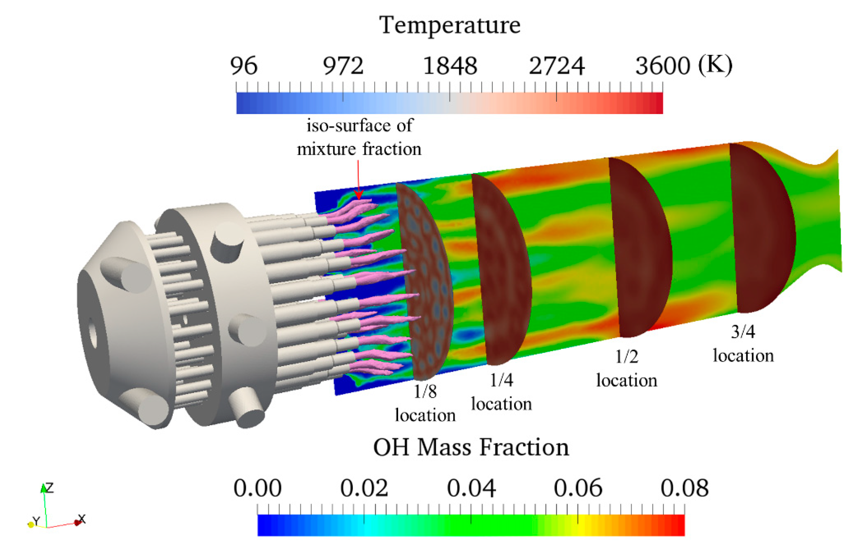
4.1. Stable Combustion

In this study, two types of simulation, i.e., stable combustion and combustion instability simulations are performed. The stable combustion analysis is focused on injector A, as shown in Figure 6, and the combustion instability analysis is focused on injector B. Unlike a perimetric injector, such as injector B, the position of injector A can suppress the flame deformation caused by a strong recirculation flow, and thus, the original structure of the flame can be clearly observed. Therefore, it is believed that the characteristics of the flame and flow field pertaining to the stable combustion can be accurately clarified. According to the DMD analysis for the pressure field, injector B is located at the node for the 1st transverse mode and 1st and 2nd radial modes. Consequently, the location of injector B is the most affected by the combustion instability and exhibits the highest Rayleigh index [20]. Therefore, it is considered that the characteristics of the flame and flow structure for the combustion instability and the corresponding difference with the stable combustion case can be accurately observed. When combustion instability occurs, the flame generally tends to be shortened, and thus, the analysis plane of injector B is half the size of that of injector A, as shown in Figure 6.
Before investigating the individual injector in the stable combustion condition, the entire flow field is investigated. Figure 7 shows the temperature contours at each axial location of the combustor, longitudinal slice contour of the OH mass fraction, and iso-surface for the mixture fraction value of 0.004. The disappearance of the oxygen core and flame development over the entire flow field are examined. The four axial locations correspond to 1/8, 1/4, 1/2, and 3/4 the length of the combustion chamber. At the 1/8 location, the temperature contour shows that the oxygen core is slightly diffused but intact. In contrast, starting from the 1/4 location, the oxygen core almost disappears, and the flame is almost homogeneous at the 1/2 and 3/4 locations. The OH mass fraction contour indicates that the mass fraction begins to develop after the 1/8 location. In this region, the oxygen core begins to mix with the hydrogen and disappears, and the OH mass fraction region begins to develops in the downstream region after this disappearance. Both the mixture fraction iso-contour and OH mass fraction contour indicate that the flame begins to expand near the 1/16 location because the specific volume of the flame increases rapidly when the mixture fraction value ranges from 0–0.004. To perform a quantitative analysis, the change in the spatially averaged temperature and pressure in the combustion chamber according to the flow time are investigated. Because the relevant experiment data for the LP4 condition are not available, the simulation results are compared with the data of previous simulations [38]. The temperature and pressure errors between the two studies are 3.6% and 6.8%, respectively, which are relatively small error values.
Figure 8 shows the instantaneous temperature, x-velocity, oxygen mass fraction, y-vorticity, and heat release rate for injector A. Figure 8a shows the flame structure. From the injector lip, the hydrogen and oxygen begin to react, leading to an attached flame. The flame expands slightly in the radial direction at a distance of x / d H 2 = 2, and cold oxygen jet is present in the center with a length of approximately l O 2 / d H 2 = 14. This oxygen core gradually disappears owing to the mixing with the shear layer and recirculation flow. Therefore, the flame is elongated and extends to the downstream region. Figure 8b shows that the hydrogen jet with a high velocity of 450 m/s is discharged from the injector exit. The recirculation flow regions are developed above and below the jet due to the high speed of the hydrogen jet. During stable combustion, the pattern of this jet is maintained. As shown in Figure 8c, the oxygen jet extends to the downstream region. The jet length is approximately l O 2 / d H 2 = 14. In addition, strong vorticity layers appear above and below the oxygen jet due to the strong hydrogen injection. Each shear layer is composed of smaller child vortices. In the region which the oxygen jet expands slightly, the shear layer is bent in the radial direction. The child vortices are distributed along the shear layers and produce a large heat release rate (with a maximum value exceeding 8 × 10⁹ W/m3) in the region in which oxygen and hydrogen are in contact.

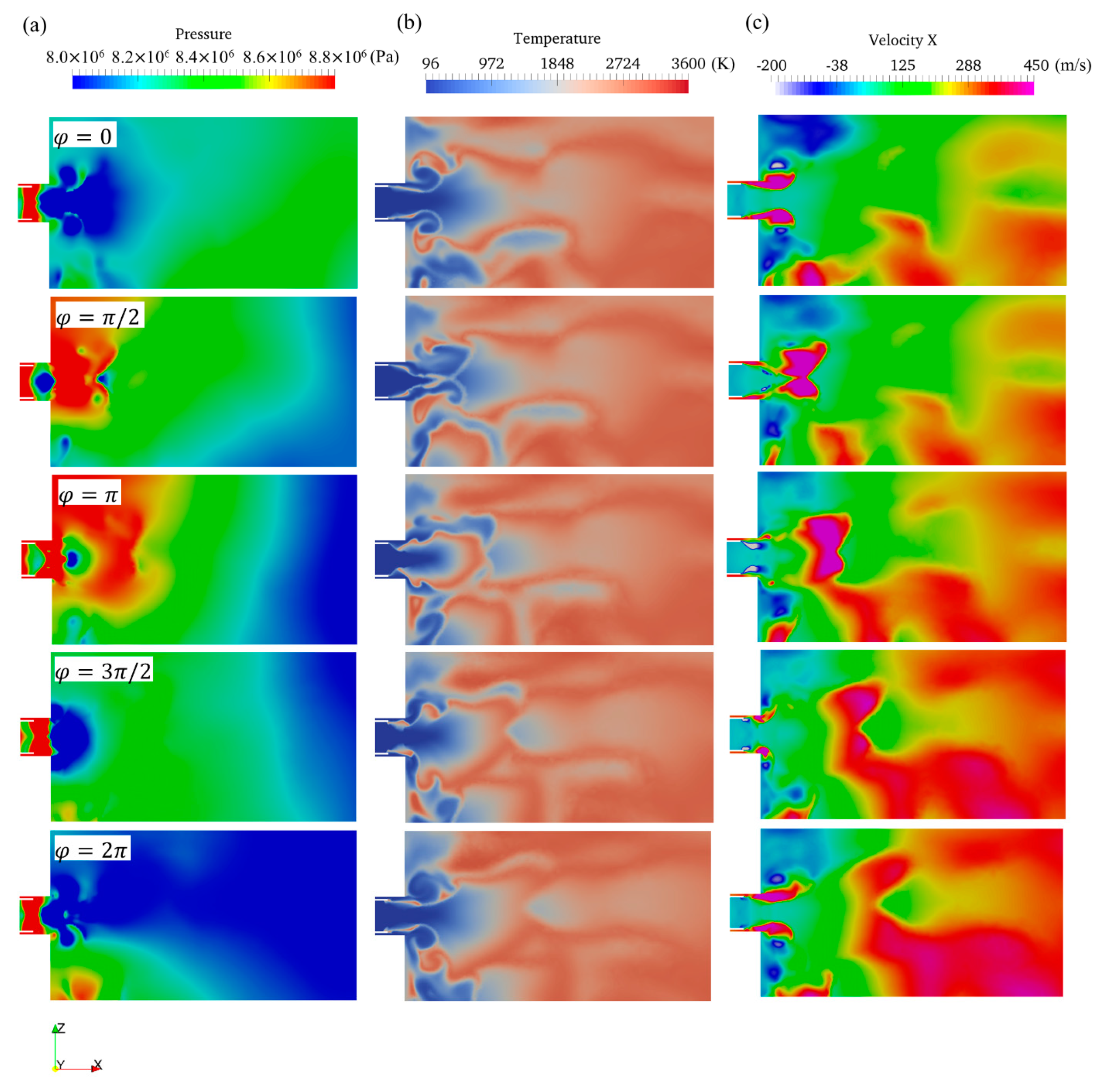
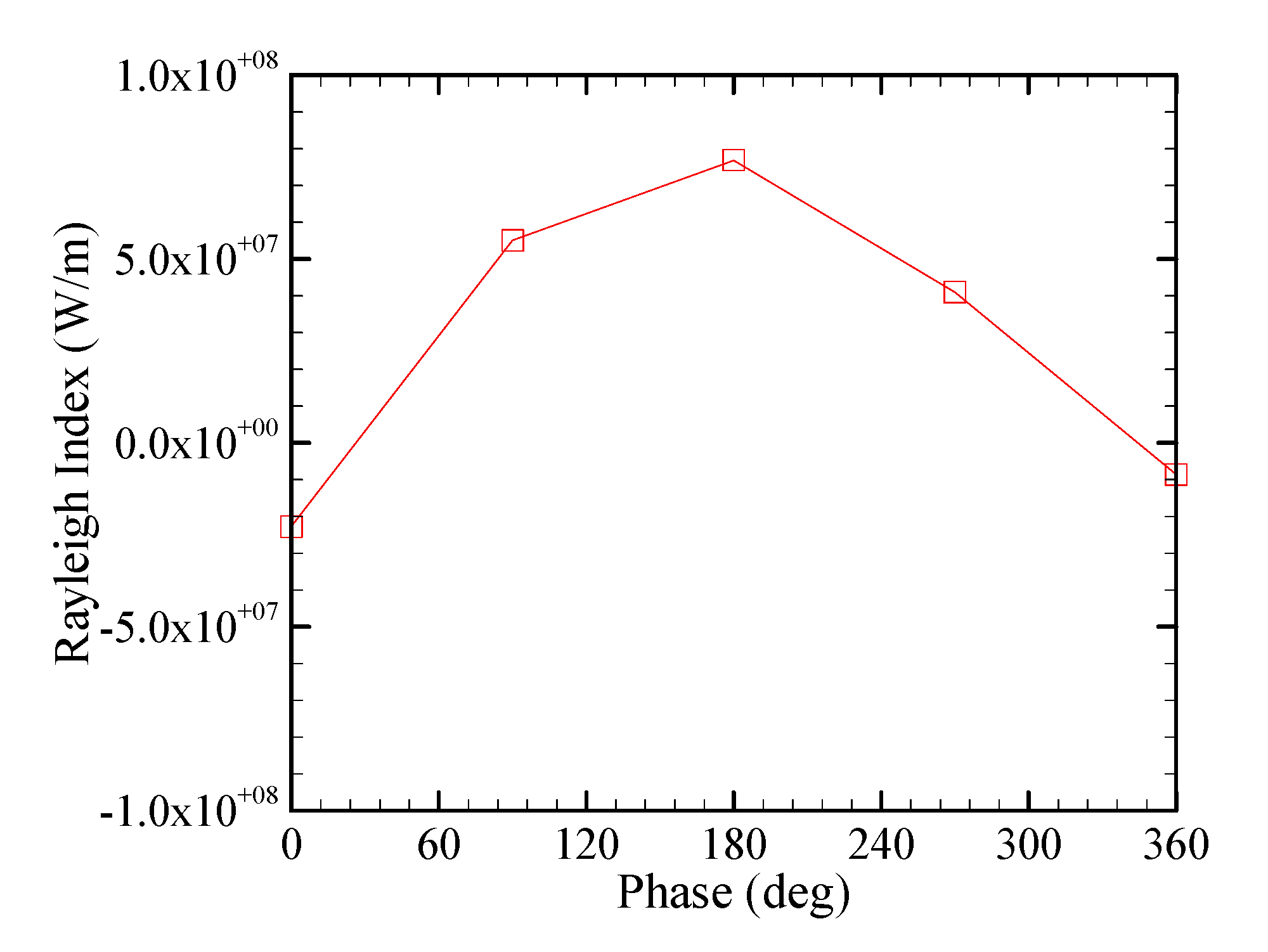
4.2. Combustion Instability

In the LP4 condition of the BKD combustor, combustion instability occurs spontaneously during the operation. However, a coarse cell size of the grid system used in the present study is not sufficient to realize the spontaneous combustion instability; therefore, it is necessary to artificially trigger the combustion instability. Nonlinear triggering can be achieved by artificially superimposing the 1st transverse standing wave solution shown in Figure 9 onto the stable combustion solution. The exact 1st transverse standing wave solution for pressure can be derived from the wave equation in a polar coordinate as in Equation (20) [39].
p ( r , θ ) = 2 M J 1 ( α 10 r R ) cos ( θ )
where M is the amplitude of mode, J 1 is the Bessel function of order n, α 10 is the abscissa of (m + 1)th extremum of the Bessel function of order n, and R is radius of cylinder, respectively.
To determine the amplitude of the standing wave solution that can sustain the combustion instability, the standing wave solutions with amplitudes corresponding to 11%, 13%, 15%, 17%, and 19% of the pressure (80 bar) of the LP4 condition are superimposed onto the stable combustion solution. As a result, the standing wave solution with the amplitude of 19% corresponding to Δ p = 1.52 × 10⁶ Pa, as shown in Figure 9, can sustain the combustion instability while the other amplitudes damp out.
The pressure history measured at the probe point (shown in Figure 9) throughout the simulation is shown in Figure 10. As shown in Figure 10a, the stable combustion reaches the steady state at 4 ms and continues until the triggering point at 10 ms. From 10 ms to 16 ms, the limit cycle is maintained by the combustion instability. Figure 10b shows the FFT result for the pressure history measured during the combustion instability simulation. Many resonant frequencies can be observed, among which, the amplitudes of the frequencies for 10.5, 21.5, 24.2, and 45.2 kHz are relatively large, as shown in Figure 10b. The frequency of 24.2 kHz corresponds to the largest amplitude. The short-time Fourier transform (STFT), which is a sequence of Fourier transforms of a windowed signal applied in the previous study [40], results shown in Figure 11 demonstrate that the frequencies 10.5, 21–24, and 45.2 kHz exhibit a large amplitude during the limit cycle. Specifically, the frequency of 10.5 kHz corresponds to a strong amplitude for 10–10.3 ms; frequencies ranging from 21–24 kHz exhibit an intermediate and large amplitude for 10–12.5 ms and 13.5–16 ms, respectively; and the amplitude for the frequency of 45.2 kHz increases initially and later gradually decreases.
Furthermore, the DMD analysis for the combustion instability field is performed to identify the resonant mode structure. As shown in Figure 12a, the frequency of 10.5 kHz corresponds to the 1st transverse mode. One of the transverse mode elements is located on the injector face plate, and the other elements are located downstream of the combustion chamber. Because the damping coefficient value is ξ = 65.46, which is positive, this transverse mode is considered to be an unstable mode. As shown in Figure 12b, the frequency of 21.5 kHz corresponds to the 1st and 2nd radial modes, and the damping coefficient is ξ = 212.74, related to an unstable mode. The 2nd radial mode is attached to the injector face plate, and the two 1st radial modes are located downstream of the combustion chamber. As shown in Figure 12c, the frequency of 24.2 kHz corresponds to the 2nd radial mode, and the damping coefficient is ξ = 108.28. This mode exists on only the injector face plate side. As shown in Figure 12d, the frequency of 45.2 kHz exhibits the 2nd radial mode, and the damping coefficient is ξ = 166.14. This mode also exists on the injector face plate side. For all the resonant modes, injector B is located at the pressure node, and thus, its location is the most affected by the strong pressure fluctuations.
The changes in the pressure, temperature, x-velocity, oxygen mass fraction, y-vorticity, and heat release rate caused by the instability modes for one period of the limit cycle are shown in Figure 13 and Figure 14. At the phase φ = 0, a low-pressure region is formed around x / d H 2 = 1–2 from the injector exit, as shown in Figure 13a. Consequently, the hydrogen is injected at a high velocity from the hydrogen injector exit, as shown in Figure 13c. This hydrogen jet forms a strong vortex with an intensity exceeding 1 × 10⁶ /s as it flows along the surface of the oxygen jet injected earlier, as shown in Figure 14. This vorticity causes the hydrogen and oxygen to be closer to each other, thereby generating a large heat release rate exceeding 1 × 10¹⁰ W/m3 in the shear layer between the hydrogen and oxygen, as shown in Figure 14. This heat release rate is several times greater than that of the stable combustion. As the pressure starts to rise at the phase φ = π/2, a high-pressure region develops around x / d H 2 = 1–2, as shown in Figure 13a. Consequently, the hydrogen jet injection is cut off, and the lump of the initially injected hydrogen jet pushes the previously injected oxygen jet downstream, as shown in Figure 13c. A large heat release rate is induced continuously on this contact surface between the oxygen and hydrogen, as shown in Figure 14. Eventually, the oxygen jet is cut off due to the strong vorticity, as shown in Figure 14. Subsequently, the flame becomes short and closed, as shown in Figure 13b. At the phase φ = π, the pressure reaches the maximum value, and the hydrogen jet injection is almost blocked. At the exit of the injector, the oxygen jet starts to be sucked downstream, as shown in Figure 14. Simultaneously, the flame begins to discharge from the injector exit, as shown in Figure 13b. The lump of hydrogen jet that pushes the lump of oxygen jet forward spreads wide, and thus, the heat release rate decreases, as shown in Figure 14. At the phase φ = 3π/2, the pressure decreases, and a low-pressure area is regenerated, as shown in Figure 13a. The hydrogen jet begins to be weakly injected, and the lumps of the hydrogen and oxygen jets in the downstream region spread wide; consequently, the corresponding concentrations and velocities decrease, and the heat release rate decreases in the downstream region. although its magnitude inside the injector remains high, as shown in Figure 14. The flame is the largest in the case shown in Figure 13b; nevertheless, the flame is as large as x / d H 2 = 1–2, shorter and wider than the flame in the stable combustion case, as shown in Figure 8a. At the phase φ = 2π, the pressure reduces to the minimum value, and the hydrogen jet is rapidly injected. The same process is repeated.
The injection of the hydrogen and oxygen jets exhibits an inverse relationship with the pressure rise, as shown in Figure 15. The graph shows the change in the pressure, x-velocity of the propellants, and heat release rate at the injector exit over multiple periods of cycles. At the maximum pressure, the velocities of the two jets decreases to the minimum value; thus, the phase difference between the injection and pressure rise is π. The phase difference between the heat release rate and pressure is sufficiently small for them to be considered to be in phase.
The Rayleigh index (RI), as defined in Equation (21), can be used to interpret the energy disturbance caused by the combustion, which is the source term of the disturbance energy transport equation.
R I = 1 τ k 1 k p ¯ τ φ p ( t ) q ( t )   d t    
where τ is the acoustic period, k is the heat specific ratio, and p ¯ is the time-averaged pressure. When the RI is positive, acoustic energy is augmented to act as an energy source that can sustain the combustion instability. As shown in Figure 16, at the phase φ = 0, the hydrogen jet is injected at a high velocity, and a large heat release rate is instantaneously induced in front of the injector exit at the hydrogen–oxygen shear layer. However, a large negative RI occurs along the shear layer because a low-pressure region is formed. Subsequently, at the phase φ = π/2, a high-pressure region begins to develop, and simultaneously, a large positive RI occurs on the contact surface of the lumps of the hydrogen and oxygen jets and near the injector exit. At the phase φ = π, a medium-intensity positive RI occurs due to the wide high-pressure region and the heat release rate distributed along the flame edge. At the phase φ = 3π/2, a large positive RI is sustained inside the injector, and a negative RI is generated at the injector exit due to the developed low-pressure region; moreover, the hydrogen jet injection begins to discharge again.
The average RI over a period is shown in Figure 17. It can be noted that the positive and negative RI regions are mixed and distributed over the flame area. The negative RI region is concentrated in the hydrogen jet injection area, and the positive RI region is widely distributed along the injector lip and edge of the flame.
The variation in the RI in the analysis plane of injector B in one period is shown in Figure 18. In the pressure drop phases, a negative RI (max. −2 × 10⁷ W/m3) is maintained for a short time; however, in the pressure rise phases, a positive RI (max. 8 × 10⁷ W/m3) is maintained for a long time. In the analysis plane of injector B, the time-averaged RI for one period is calculated as +243,156 W/m3.

5. Conclusions

A numerical simulation to analyze the turbulent combustion and combustion instability is performed on a H2-O2 liquid rocket combustor with 42 shear-coaxial injectors. The simulation is performed based on SLFMFoam_LES, a newly developed OpenFOAM-based turbulent reacting flow solver for a real-gas combustion. This solver combines the flow solver based on the PIMPLE algorithm and SLFM approach, and is capable of a LES of turbulent combustion. Because the combustor operates in a high-pressure condition, the RK–PR equation is employed as a real-gas equation model.
First, the numerical simulation for the entire field and a single injector representing all the injectors is performed to understand the general flow and flame characteristics in the stable combustion condition. In the analysis, the temperature, x-velocity, mass fraction, vorticity and heat release rate are investigated. The flame appears to be nearly constant over time without any periodic changes. The flame expands slightly at a distance of approximately x / d H 2 = 2 from the exit of the injector, and the oxygen jet is slowly vanished through mass diffusion and turbulent diffusion, with the jet being present in the far downstream region. The flame is elongated from the injector lip to the downstream region of the combustor. The shape of the hydrogen jet injection and position of the vortices distributed along the velocity shear layer do not change significantly with time.
For the combustion instability analysis, to artificially trigger the combustion instability, the 1st transverse standing wave solution is created and superimposed on the stable combustion solution. The wave solutions with an amplitude equivalent to 11–19% of the pressure of the stable combustion are created, and the triggering tests are conducted. It is noted that the combustion instability occurs at the 19% case.
The eigen-frequencies and eigen-modes are investigated through FFT and DMD to confirm the occurrence of the combustion instability. Four representative unstable frequencies (10.5, 21.5, 24.2, 45.7 kHz) are observed, and the shapes of the unstable modes are evaluated. The unstable 1T mode is observed at f = 10.5 kHz, unstable 1R and 2R modes are observed at f = 21.5 kHz, unstable 2R mode is observed at f = 24.2 kHz, and unstable 2R mode is observed at f = 45.7 kHz. For all the modes, injector B is located at the pressure node, and because this location is largely affected by the combustion instability, the instability analysis is performed for injector B.
Before investigating the limit cycle process, the flow and flame field changes due to the effect of the modes are investigated by phase. The temperature, pressure, x-velocity, mass fraction, vorticity, and heat release rate are examined. The structure of the flame changes periodically, and therefore, the flame repeatedly vanishes and expands near the injector exit. The flame size is considerably smaller compared to that of the stable combustion flame.
In the pressure rise section, the injection of the hydrogen jet is suppressed, and the heat release rate increases downstream due to the reaction between the lumps of the hydrogen and oxygen jets. In the pressure drop section, the injection of the hydrogen jet becomes intense, and the heat release rate increases in front of the injector exit. The pressure, x-velocity, and heat release rate are plotted in one period of the cycles at the injector exit, and the correlation among these parameters is confirmed.
Based on these observations, the RI is evaluated to understand the sustenance process of the limit cycle. In the section in which the pressure rises, the RI is mainly positive throughout the analysis plane of injector B. The positive region is distributed downstream wherein the lumps of the hydrogen and oxygen jets react, and in certain cases, the positive region is located along the flame edge when the flame expands to its maximum size.
The RI is generally negative in the pressure drop section. The negative region is distributed along the high-velocity hydrogen jet injection. The phase-averaged RI shows that the positive and negative regions are mixed throughout the flame field, although the positive region is slightly dominant overall. The investigation of the RI for each phase indicates that, in general, the negative RI is maintained for a short time in the pressure drop section, and the positive RI is maintained for a long time in the pressure rise section. Therefore, overall, the positive RI is dominant indicating the sustenance condition of the limit cycle.

Author Contributions

Conceptualization, J.-Y.C., W.-S.H.; Data curation, W.-S.H., B.-K.S. and B.J.L.; methodology, W.H., K.Y.H., B.J.L., H.S.H., C.H.S.; investigation, W.-S.H., W.H., K.Y.H., B.J.L., H.S.H., C.H.S.; writing—original draft preparation, W.-S.H.; writing—review and editing, J.-Y.C.; visualization, W.-S.H.; supervision, J.-Y.C.; project administration, J.-Y.C.; funding acquisition, J.-Y.C. All authors have read and agreed to the published version of the manuscript.

Funding

This research received no external funding.

Informed Consent Statement

Not applicable.

Acknowledgments

This work was supported by the Space Core Technology Research Grants (2017M1A3A3A03015445) and Basic Science Research Program Grant (2019R1A2C1004505) through the National Research Foundation (NRF) of Korea, funded by the Ministry of Science and ICT (MSIT) of the Republic of Korea Government.

Conflicts of Interest

The authors declare no conflict of interest.

Nomenclature

A: B: Ccoefficients of the quadratic equation of ksgs
acenergy parameter of the RK–PR equation
bsize-related parameter of the RK–PR equation
ddiameter, m
ffrequency, Hz
kturbulent kinetic energy or specific heat ratio, m2/s2
ljet length, m
nparameter defining the temperature dependence of the attractive term of RK–PR equation
m ˙ mass flow rate, kg/s
ppressure, Pa or bar
Pprobability density function
Runiversal gas constant, J/kg·mol
RIRayleigh index
SijStrain rate tensor, 1/s
ScSchmidt number
Ttemperature, K
Trreduced temperature
ttime, s
uivelocity component, m/s
vmolar volume, m3/mol
Vvolume, m3/kg
xiCartesian coordinate, m
ynormal distance to a wall, m
Ymolar fraction of species
zmixture fraction
z”2mixture fraction variance
Zccritical compressible factor
Δfilter cutoff length, m
α, β, γparameters of β-pdf
Γgamma function
δijKronecker delta
δ1third parameter of RK–PR equation
εeddy dissipation rate, m2/s3
μabsolute viscosity, N·s/m2
ρdensity, kg/m3
τacoustic period
τijstress tensor, N/m2
χscalar dissipation rate, 1/s
ωacentric factor
Subscripts
ccombustion chamber
crcritical point
i, jCartesian direction
tturbulence quantity
vDvan Driest
Superscripts
sgssub-grid scale
φ phase
ϕ ¯ spatially filtered quantity or mean quantity
ϕ ˜ Favre-filtered quantity
ϕ fluctuation quantity

References

  1. Sutton, G.; Biblarz, O. Rocket Propulsion Elements; John Wiley & Sons, Inc.: New York, NY, USA, 2001. [Google Scholar]
  2. Hardi, J. Experimental Investigation of High Frequency Combustion Instability in Cryogenic Oxygen-Hydrogen Rocket Engines. Ph.D. Thesis, School of Mechanical Engineering, The University of Adelaide, Adelaide, Australia, 2012. [Google Scholar]
  3. Hardi, J.; Beinke, S.; Oschwald, M.; Dally, B. Coupling of Cryogenic Oxygen–Hydrogen Flames to Longitudinal and Transverse Acoustic Instabilities. J. Propuls. Power 2014, 30, 991–1004. [Google Scholar] [CrossRef]
  4. Gröning, S.; Oschwald, M.; Sattelmayer, T. Influence of Hydrogen Temperature on Combustion Chamber Acoustics in a LOX/H2 Rocket Engine Combustion Chamber; Sonderforschungsbereich/Transregio 40—Annual Report 2013: Semantic Scholar: Seattle, WA, USA, 2013; pp. 199–211. [Google Scholar]
  5. Gröning, S.; Suslov, J.; Hardi, J.; Oschwald, M. Influence of Hydrogen Temperature on Rocket Engine Combustion Chamber Acoustics; Sonderforschungsbereich/Transregio 40—Annual Report 2014; The German Aerospace Center: Koeln/Cologne, Germany, 2014; pp. 217–228. [Google Scholar]
  6. Armbruster, W.; Gröning, S.; Hardi, J.; Oschwald, M. Analysis of High Amplitude Acoustic Pressure Field Dynamics in a LOX/H2 Rocket Combustor; Sonderforschungsbereich/Transregio 40—Annual Report 2016; Semantic Scholar: Seattle, WA, USA, 2016; pp. 203–214. [Google Scholar]
  7. Poschner, M.M.; Pfitzner, M. Real Gas Simulation of Supercritical H2-LOX Combustion in the MASCOTTE Single-Injector Combustor Using a Commercial CFD Code. In Proceedings of the 46th AIAA 2008-952 Aerospace Science Meeting and Exhibit, Reno, NV, USA, 7–10 January 2008. [Google Scholar]
  8. Kim, T.H.; Kim, Y.M.; Kim, S.K. Real-fluid flamelet modeling for gaseous hydrogen/cryogenic liquid oxygen jet flames at supercritical pressure. J. Supercrit. Fluids 2011, 58, 254–262. [Google Scholar] [CrossRef]
  9. Coclite, A.; Cutrone, L.; Pascazio, G.; De Palma, P. Numerical Investigation of High-Pressure Combustion in Rocket Engines Using Flamelet/Progress-Variable Models. In Proceedings of the 53rd AIAA Aerospace Sciences Meeting, Kissimmee, FL, USA, 7–10 January 2008; AIAA 2015-1109. American Institute of Aeronautics and Astronautics (AIAA): Reston, VA, USA, 2015. [Google Scholar]
  10. Benmansour, A.; Liazid, A.; Logerais, P.O.; Durastanti, J.F. A 3D numerical study of LO2/GH2 supercritical combustion in the ONERA-Mascotte Test-rig configuration. J. Therm. Sci. 2016, 25, 97–108. [Google Scholar] [CrossRef]
  11. Seidl, M.J.; Aigner, M.; Keller, R.; Gerlinger, P. CFD simulations of turbulent nonreacting and reacting flows for rocket engine applications. J. Supercrit. Fluids 2017, 121, 63–77. [Google Scholar] [CrossRef] [Green Version]
  12. Traxinger, C.; Zips, J.; Pfitzner, M. Single-Phase Instability in Non-Premixed Flames under Liquid Rocket Engine Relevant Conditions. J. Propuls. Power 2019, 35, 675–689. [Google Scholar] [CrossRef]
  13. Schmitt, T. Large-Eddy Simulations of the Mascotte Test Cases Operating at Supercritical Pressure. Flow Turbul. Combust. 2020, 105, 159–189. [Google Scholar] [CrossRef]
  14. Hwang, W.S.; Han, W.; Huh, K.Y.; Kim, J.; Lee, B.J.; Choi, J.-Y. Numerical Simulation of a GH2/LOx Single Injector Combustor and the Effect of the Turbulent Schmidt Number. Energies 2020, 13, 6616. [Google Scholar] [CrossRef]
  15. Huang, Y.; Yang, V. Dynamics and stability of lean-premixed swirl-stabilized combustion. Prog. Energy Combust. Sci. 2009, 35, 293–364. [Google Scholar] [CrossRef]
  16. Wolf, P.; Staffelbach, G.; Roux, A.; Gicquel, L.; Poinsot, T.; Moureau, V. Massively parallel LES of azimuthal thermo-acoustic instabilities in annular gas turbines. C. R. Mec. 2009, 337, 385–394. [Google Scholar] [CrossRef]
  17. Wolf, P.; Balakrishnan, R.; Staffelbach, G.; Gicquel, L.; Poinsot, T. Using LES to Study Reacting Flows and Instabilities in Annular Combustion Chambers. Flow Turbul. Combust. 2012, 88, 191–206. [Google Scholar] [CrossRef] [Green Version]
  18. Srinivasan, S.; Ranjan, R.; Menon, S. Flame Dynamics during Combustion Instability in a High-Pressure, Shear-Coaxial Injector Combustor. Flow Turbul. Combust. 2015, 94, 237–262. [Google Scholar] [CrossRef]
  19. Schulze, M.; Zahn, M.; Schmid, M.; Sattelmayer, T. About Flame-Acoustic Coupling Phenomena in Supercritical H2/O2 Rocket Combustion Systems. In Proceedings of the Deutscher Luft-und Raumfahrtkongress, Augsburg, Swabia, Bavaria, Germany, 16–18 September 2014. DocumentID: 340018. [Google Scholar]
  20. Urbano, A.; Selle, L.; Staffelbach, G.; Cuenot, B.; Schmitt, T.; Ducruix, S.; Candel, S. Exploration of combustion instability triggering using Large Eddy Simulation of a multiple injector liquid rocket engine. Combust. Flame 2016, 169, 129–140. [Google Scholar] [CrossRef] [Green Version]
  21. Urbano, A.; Douasbin, Q.; Selle, L.; Staffelbach, G.; Cuenot, B.; Schmitt, T.; Ducruix, S.; Candel, S. Study of flame response to transverse acoustic modes from the LES of a 42-injector rocket engine. Proc. Combust. Inst. 2016, 36, 2633–2639. [Google Scholar] [CrossRef] [Green Version]
  22. Schmitt, T.; Staffelbach, G.; Ducruix, S.; Gröning, S.; Hardi, J.; Oschwald, M. Large-Eddy Simulations of a Sub-Scale Liquid Rocket Combustor: Influence of Fuel Injection Temperature on Thermo-Acoustic Stability. In Proceedings of the 7th European Conference for Aeronautics and Aerospace Science (EUCASS), Milan, Italy, 3–6 July 2017. [Google Scholar]
  23. Smagorinsky, J. General Circulation Experiments with the Primitive Equations I. The Basic Experiment. Mon. Weather Rev. 1963, 91, 99–164. [Google Scholar] [CrossRef]
  24. OpenFOAM: User Guide v2006. Available online: https://www.openfoam.com/documentation/guides/latest/doc/guide-turbulence-les-smagorinsky.html (accessed on 1 December 2020).
  25. Faghri, A.; Zhang, Y.; Howell, J.R. Advanced Heat and Mass Transfer; Global Digital Press: Columbia, MO, USA, 2010; pp. 420–421. [Google Scholar]
  26. Cismondi, M.; Mollerup, J. Development and application of a three-parameter RK–PR equation of state. Fluid Phase Equilibria 2005, 232, 74–89. [Google Scholar] [CrossRef]
  27. Soave, G. Equilibrium constants from a modified Redlich-Kwong equation of state. Chem. Eng. Sci. 1972, 27, 1197–1203. [Google Scholar] [CrossRef]
  28. Peng, D.-Y.; Robinson, D.B. A New Two-Constant Equation of State. Ind. Eng. Chem. Fundam. 1976, 15, 59–64. [Google Scholar] [CrossRef]
  29. Liu, F.; Guo, H.; Smallwood, G.J.; Gülder, Ö.L.; Matovic, M.D. A robust and accurate algorithm of the β-pdf integration and its application to turbulent methane–air diffusion combustion in a gas turbine combustor simulator. Int. J. Therm. Sci. 2002, 41, 763–772. [Google Scholar] [CrossRef]
  30. Triantafyllidis, A.; Mastorakos, E. Implementation Issues of the Conditional Moment Closure Model in Large Eddy Simulations. Flow Turbul. Combust. 2010, 84, 481–512. [Google Scholar] [CrossRef]
  31. Conaire, M.Ó.; Curran, H.J.; Simmie, J.M.; Pitz, W.J.; Westbrook, C.K. A comprehensive modeling study of hydrogen oxidation. Int. J. Chem. Kinet. 2004, 36, 603–622. [Google Scholar] [CrossRef]
  32. Chen, K.K.; Tu, J.H.; Rowley, C.W. Variants of Dynamic Mode Decomposition: Connections between Koopman and Fourier Analyses. J. Nonlinear Sci. 2012, 22, 887–915. [Google Scholar] [CrossRef]
  33. Schmid, P.J. Dynamic mode decomposition of numerical and experimental data. J. Fluid Mech. 2010, 656, 5–28. [Google Scholar] [CrossRef] [Green Version]
  34. Hakim, L.; Schmitt, T.; Ducruix, S.; Candel, S. Dynamics of a transcritical coaxial flame under a high-frequency transverse acoustic forcing: Influence of the modulation frequency on the flame response. Combust. Flame 2015, 162, 3482–3502. [Google Scholar] [CrossRef]
  35. Caretto, L.S.; Gosman, A.D.; Patankar, S.V.; Spalding, D.B. Two Calculation Procedures for Steady, Three-Dimensional Flows with Recirculation. In Proceedings of the Third International Conference on Numerical Methods in Fluid Mechanics; Volume 19 of Lecture Notes in Physics; Cabannes, H., Temam, R., Eds.; Springer: Berlin, Germany, 1972; pp. 60–68. [Google Scholar]
  36. Issa, R.I. Solution of the implicitly discretised fluid flow equations by operator-splitting. J. Comput. Phys. 1986, 62, 40–65. [Google Scholar] [CrossRef]
  37. Roe, P.L. Characteristic-Based Schemes for the Euler Equations. Annu. Rev. Fluid Mech. 1986, 18, 337–365. [Google Scholar] [CrossRef]
  38. Hwang, W.S.; Han, W.; Huh, K.Y.; Goo, S.; Lee, B.J.; Choi, J.Y. Numerical Simulation of a GH2/LOX Rocket Combustor with Multiple Injectors Using Real Gas Flamelet Model. In Proceedings of the AIAA 2019-4293 Propulsion and Energy 2019 Forum, Indianapolis, IN, USA, 19–22 August 2019. [Google Scholar]
  39. Sliphorst, M.; Gröning, S.; Oschwald, M. Theoretical and Experimental Identification of Acoustic Spinning Mode in a Cylindrical Combustor. J. Propuls. Power 2011, 27, 182–189. [Google Scholar] [CrossRef]
  40. Jeong, S.M.; Choi, J.Y. Combined Diagnostic Analysis of Dynamic Combustion Characteristics in a Scramjet Engine. Energies 2020, 13, 4029. [Google Scholar] [CrossRef]
Figure 1. Geometry and components of the DLR-BKD combustor, with the arrangement of the injectors shown in the upper right corner.
Energies 14 00419 g001
Figure 2. Grid overview with close-up view of the injection region along with the location of the probe to measure the turbulent kinetic energy (TKE) signal.
Energies 14 00419 g002
Figure 3. Comparison of the frequency spectrum of TKE with Kolmogorov’s −5/3 law.
Energies 14 00419 g003
Figure 4. Process flow of the SLFMFoam_LES solver algorithm.
Energies 14 00419 g004
Figure 5. Plots of the mixture fraction verses (a) temperature, (b) density from generated flamelet table. The x-axis of the zoomed-in frame in plot (b) is reset to 0–0.004. The range of scalar dissipation rate (SDR) for both plots is 105–50,000.
Energies 14 00419 g005
Figure 6. Longitudinal and transverse slice plots of the instantaneous temperature field with the analysis planes of injectors A and B for the stable combustion and combustion instability analysis, respectively.
Energies 14 00419 g006
Figure 7. Transverse slice contours of the temperature at four axial locations, longitudinal slice contour of OH mass fraction, and iso-surface of the mixture fraction value of 0.004 (represented in pink).
Energies 14 00419 g007
Figure 8. Contour plots of instantaneous (a) temperature, (b) x-velocity, (c) oxygen mass fraction and y-vorticity with iso-contour of the heat release rate in the analysis plane of injector A under the stable condition.
Energies 14 00419 g008
Figure 9. Exact 1st transverse standing wave solution generated on the DLR-BKD combustion chamber with the probe point to measure the pressure history.
Energies 14 00419 g009
Figure 10. Plots of the (a) pressure history and (b) fast Fourier transform (FFT) result of the pressure history during combustion instability.
Energies 14 00419 g010
Figure 11. The short-time Fourier transform (STFT) result during combustion instability.
Energies 14 00419 g011
Figure 12. Resonant modes decomposed from the DMD method, (a) unstable 1st transverse mode (f = 10.5 kHz), (b) unstable 1st and 2nd radial modes (f = 21.5 kHz), (c) unstable 2nd radial mode (f = 24.2 kHz), (d) unstable 2nd radial mode (f = 45.2 kHz).
Energies 14 00419 g012
Figure 13. Contour plots of the (a) pressure, (b) temperature, (c) x-velocity according to the phase changes for the analysis plane of injector B in one period of the cycles.
Energies 14 00419 g013
Figure 14. Contour plots of the oxygen mass fraction, y-vorticity with the iso-surface of the heat release rate according to the phase change for the analysis plane of injector B during one period of the cycles.
Energies 14 00419 g014
Figure 15. Plot of the pressure, x-velocity of oxygen, and x-velocity of hydrogen, and heat release rate comparison according to the phase change during multiple periods of the cycles at the injector exit.
Energies 14 00419 g015
Figure 16. Iso-surface of the Rayleigh index by phase change at the analysis plane of injector B in one period of the cycles, overlapped with the oxygen and hydrogen mass fraction contours.
Energies 14 00419 g016
Figure 17. Phase-averaged Rayleigh index in the analysis plane of injector B for one period of the cycles.
Energies 14 00419 g017
Figure 18. Rayleigh index averaged spatially over the analysis plane of injector B verses the phase in one period of the cycles.
Energies 14 00419 g018
Table 1. Propellant supply conditions and theoretical estimate values.
O/F Ratio m ˙ H 2 ( kg / s ) m ˙ O 2 ( kg / s ) T H 2 ( K ) T O 2 ( K ) p H 2 ( MPa ) p O 2 ( MPa ) p c ( MPa ) T c ( K )
6.00.965.759611110.39.48.03627
Publisher’s Note: MDPI stays neutral with regard to jurisdictional claims in published maps and institutional affiliations.

