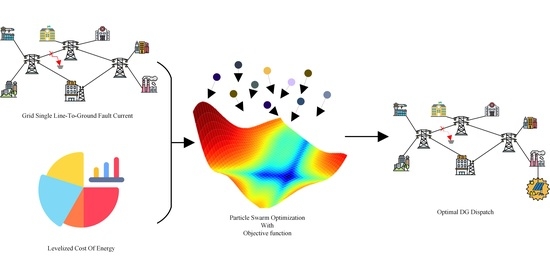
The Optimal Allocation of Distributed Generators Considering Fault Current and Levelized Cost of Energy Using the Particle Swarm Optimization Method

Abstract

The power requirements of grids have risen as artificial intelligence and electric vehicle technologies have been used. Thus, the installation of distributed generators (DGs) has become an essential factor to streamline power grids. The objective of this study is to optimize the capacity and location of DGs. For this purpose, an objective function was defined, which takes into account the fault current and the levelized cost of energy, and a modified particle swarm optimization method was applied. Then, we analyzed a case of a single line-to-ground fault with a test feeder (i.e., the IEEE 30 bus system) with no DGs connected, as well as a case where the DGs are optimally connected. The effect of the optimally allocated DGs on the system was analyzed. We discuss an optimal layout method that takes the economic efficiency of the DG installation into account.

1. Introduction

Classical unsymmetrical fault analysis is based on node equations and sequence network and was presented by Kimbark in 1946 [1]. These methods were also presented by Anderson and Kundur [2,3]. Many modern fault analysis and control methods that are model or signal based [4] are presented by many researchers. The application of new technologies such as artificial intelligence and electrical vehicles has increased the burden of power grids. Modern distributed generators (DGs) have an ability to reduce the burden by injecting active power and reactive power based on power electronics [5].

Recently, fault diagnosis methods based on convolutional neural networks [6], Bayesian networks [7], and support vector machines [8] were also presented. Modern DG installation-cost optimization methods based on supervisory control and data acquisition (SCADA), hardware-in-the-loop [9], and power-flow management systems [10] were presented by researchers. A standard guideline for connecting DGs to a grid was presented by IEEE [11]. This guideline suggests connecting DGs as current sources. That is, when a fault occurs, DGs inject current. Thus, the fault current should be taken into account for the problem of DG installation optimization.

These previous methods of fault diagnosis and DG installation optimization have demonstrated the possibilities of more complex systems being analyzed by system data, including DGs. However, none of the previous studies have optimized the location and capacity of DGs with an objective function that takes into account not only the short-circuit current of DGs that act as a current source, but also the levelized costs. Thus, in this paper, we present a method to calculate the single line-to-ground fault current at a test feeder (e.g., the IEEE 30 bus system). Based on the fault current, we optimize the location of DGs while considering the levelized cost of energy (LCOE) using particle swarm optimization (PSO). A proper objective function for the PSO method was selected by examining the various objective functions and comparing their performance indices.

According to Sörensen and Glover’s definition, a metaheuristic algorithm is a high-level algorithmic and problem-independent framework for developing heuristic algorithms [12]. The purpose of a metaheuristic algorithm is to find a near-optimal solution with reasonable computational cost [13]. Most metaheuristic algorithms such as particle swarm optimization (PSO), the genetic algorithm (GA), and ant colony optimization are inspired by nature [14]. Such algorithms are widely used to solve optimization problems. According to the literature, PSO and GA are highly popular for solving DG allocation problems [15,16,17,18].

In this study, PSO was used because it gives better solution quality and takes a smaller number of iterations than GA [19]. The major advantages of the PSO method are the implementation simplicity, fast convergence, short computation time, and high efficiency in finding the global optima [19]. Thus, in this study, we present a method for accurate DG allocation that calculates single line-to-ground fault current in a test feeder. Based on the fault current, we optimize the location and capacity of DGs while considering the LCOE using the PSO algorithm. A proper objective function for the PSO method was also selected by examining the various objective functions and comparing their performance indices.

The rest of this study is organized as follows. Section 2 presents the problem statement. In Section 3, we discuss the definition of DGs, their modeling, and the fault analysis method and present a case study to show how much DGs affect the fault current. Next, Section 4 presents the proposed methods. Section 5 presents the detailed optimization method and the results. Finally, in Section 6 and Section 7, we discuss our research and summarize our conclusions.

2. Problem Statement

In this study, we consider a method for connecting DGs with their optimal capacity in their optimal locations. For this research, the fault current was determined in the IEEE 30-bus system, which is a test feeder system used by researchers to implement new optimization studies. The fault current level and the LCOE are equally weighted in the objective function. In addition to the weight in the objective function, various well-known objective functions were evaluated through performance indices in order to find the optimal objective function. A PSO method is presented using the objective function including the fault current and the LCOE for the optimal allocation of DGs. The performance of the PSO method was compared to that of a GA.

3. Distributed Generators and Their Fault Analysis

3.1. Distributed Generators

DGs offer many advantages to power systems. For example, they contribute to lowering greenhouse gas emissions because they promote clean power generation [20]. They are also based on renewable energy, enabling sustainable urban designs. Thus, DGs provide technical, economic, and environmental benefits [20].

Grids are usually as complex as cobwebs. A grid to which a DG is connected becomes a more complex system. In these situations, technical problems such as an increase in short-circuit currents, the selectivity of the protection system, and the perturbation of voltage levels often occur [21]. DGs can be classified as:

• Rotational DGs such as wind power and gas turbines;
• Stationary DGs using inverters such as solar power and variable-speed wind power.

When as more loads and equipment are connected to the grid, classical power systems generally deliver power from conventional centralized power plants (e.g., coal, gas, and nuclear power stations) to users. However, these systems may not effectively solve energy problems such as abrupt increases in power injected by DGs, worsening power quality, or complex interactions with the energy market. To relieve these problems, a method of optimally connecting the DGs to the grid can be used.

3.2. Distribution Generator Modeling Method

Distributed generators are sometimes connected to the grid as either a voltage or current source. To analyze the effect of faults of DGs on the grid, DGs should be modeled in one of these two ways.

3.2.1. Voltage Source

In Figure 1, rotational machine-based DGs (e.g., synchronous generators) can be modeled as a voltage source in the short-circuit study [22]. For example, the DG connected to the grid in Figure 1a can be reduced into Thevenin’s equivalent circuit model (i.e., Figure 1b). That is, the DG consists of a voltage source $E_a$, or the generator interval voltage, and a source impedance $Z_s$ [23]. Thus, E_a and Z_s correspond to Thevenin’s voltage and impedance for the DG. Each fault current value is determined by solving a combination of positive-, negative-, and zero-sequence networks [24]. Kirchhoff’s voltage law determines the terminal voltage of the DG (i.e., V_a):

$$E_a=I_a{Z}_s+V_a.$$

(1)

3.2.2. Current Source

Stationary DGs (e.g., current source inverter based DGs) can be modeled as a current source [22]. In this case, the DG is reduced into Norton’s equivalent circuit model. That is, the DG consists of Norton’s equivalent current source $I_s$ and a parallel admittance $Y_s$ [23]. These values are also derived by Thevenin’s and Norton’s source transformation theorem:

$$\frac{E_a}{Z_s}=I_a+\frac{V_a}{Z_s}=I_a+Y_s{V}_a=I_s.$$

(2)

Figure 1 shows how DGs are modeled by Thevenin’s or Norton’s equivalent circuit.

3.3. Fault Analysis

3.3.1. Unsymmetrical Electrical Fault

In a three-phase power system, the following short circuits can occur in order of frequency of occurrence: single line-to-ground (SLG), double line-to-ground (DLG), line-to-line (LL), and balanced three-phase faults. When an unsymmetrical fault occurs in the grid, the sequence networks are combined at only the faulted bus or node [24]. This means that in a pre-fault situation, each sequential network is decoupled. Figure 2 shows uncoupled general sequence networks: zero-, positive-, and negative-sequence networks.

3.3.2. General Analysis Method of Single Line-to-Ground Fault

An SLG fault that occurs at phase a in a general three-phase power grid is shown in Figure 3a. From the figure, the following is derived:

$$\left.\begin{array}{c}\mathrm{Fault} \mathrm{conditions} \mathrm{in} \mathrm{phase} \mathrm{domain}\\ \mathrm{Sin}\mathrm{gle} \mathrm{line}\text{-}\mathrm{to}\text{-}\mathrm{ground} \mathrm{fault}\end{array}\right\}\begin{array}{c}{I}_b=I_c=0\\ V_{ag}=Z_F{I}_a\hfill \end{array}$$

(3)

We transform Equation (3) to the sequence domain:

$$\left[\begin{array}{c}{I}_0\\ I_1\\ I_2\end{array}\right]=\frac{1}{3}\left[\begin{array}{ccc}1& 1& 1\\ 1& \alpha & {\alpha }^2\\ 1& {\alpha }^2& \alpha \end{array}\right]\left[\begin{array}{c}{I}_a\\ 0\\ 0\end{array}\right]=\frac{1}{3}\left[\begin{array}{c}{I}_a\\ I_a\\ I_a\end{array}\right], \alpha =1\angle {120}^{°}.$$

(4)

By using Fortescue’s theorem,

$$\left(V_0+V_1+V_2\right)=Z_F\left(I_0+I_1+I_2\right)$$

(5)

From Equations (4) and (5),

$$\left.\begin{array}{c}\mathrm{Fault} \mathrm{conditions} \mathrm{in} \mathrm{sequence} \mathrm{domain}\\ \mathrm{Sin}\mathrm{gle} \mathrm{line}\text{-}\mathrm{to}\text{-}\mathrm{ground} \mathrm{fault}\end{array}\right\}\begin{array}{c}{I}_0=I_1=I_2\\ \left(V_0+V_1+V_2\right)=3Z_F{I}_1\end{array}$$

(6)

Equation (6) can be satisfied by connecting the sequence networks in series at the fault point through the fault impedance $3Z_F$, as shown in Figure 3b. From this figure, the sequence components of the fault currents are:

$$I_0=I_1=I_2=\frac{V_F}{Z_0+Z_1+Z_2+3Z_F}$$

(7)

3.4. Short-Circuit Current Calculation Example

To verify the impact on the fault current when a DG is connected to the grid, a small 5-bus power system with a base of 100 MVA was modeled. The grid has a slack generator at bus 1 and a three-winding transformer connected in a wye-delta-grounded wye between buses 1 and 2 and lines in buses 2, 3, and 4. There is a step-down transformer between buses 4 and 5 connected in a ground wye-delta. An inverter-based distributed generator (IBDG) is connected to bus 5 with a capacity of 10 MVA. These are illustrated in Figure 4.

For confirming the impact of the DG on the fault current, this study assumes that an SLG fault occurs at bus 3 in Figure 4. Also, we suppose an IBDG is connected to the system as a current source. Many technical standards suggest connecting DGs to the grid as a current source with grid codes [11]. When a fault occurs in the grid, Thevenin’s voltage source (i.e., a slack generator) and Norton’s current source (i.e., IBDG) inject the fault current. For example, it is generally known that an IBDG contributes two times its rated current for more than a 0.5 cycle [22]. The overcurrent duration is also typically 3 to 7 cycles [25,26,27,28,29]. To model the fault current level injected by IBDGs designed as an ideal current source, Norton’s equivalent impedance, or Z_NORT = $1/Y_s$, in Figure 1 can be set as the infinite [22]. The study proposed 10⁴ p.u. as a sufficiently large value [22]. As a result of the trial and error calculations, the value decreased up to 10³ p.u. does not change the fault current in the following optimization study. Thus, we assume a Z_NORT of 10³ p.u. Figure 5 shows the situation.

3.4.1. Fault Current Contributed by a Voltage Source

To consider how much the voltage source contributes to the fault current, we assume the current source is an open circuit. This means the original fault current value occurs when the DG is not connected to the grid. This situation is illustrated in Figure 6. The fault current is calculated by Equation (8). The value of the fault current at phase a is calculated as:

$$\begin{array}{c}\frac{1}{3}{I}_{f,vs}=\frac{V_F}{Z_{33}^{+}+Z_{33}^{-}+Z_{33}^0+3Z_F}=0.3279\angle -{74.5947}^{°} [\mathrm{p}.\mathrm{u}]\\ \mathrm{Where} Z_F=0, V_F=1\angle 0^{°}\end{array}$$

(8)

$$I_{f,vs}^A=0.9837\angle -{74.5947}^{°}$$

(9)

3.4.2. Current Injection Method

If a stationary DG is connected to the grid, it works as a current source, so we need to conduct current source analyses in addition to a voltage source analysis. For such an analysis, the detailed current injection method is introduced in other studies [30,31,32]. For example, the current source is located on the transformer side of the positive-sequence circuit, so the fault current can be calculated as:

$$\frac{1}{3}{I}_{f,cs}=0.0798\angle -{3.2744}^{°} [\mathrm{p}.\mathrm{u}]$$

(10)

That is, when the DG is connected as a current source, the fault current contributed by the DG can be found by the principle of the current divider. This is illustrated in Figure 7. The fault current of phase a is calculated as:

$$I_{f,cs}^A=0.2394\angle -{3.2744}^{°} [\mathrm{p}.\mathrm{u}]$$

(11)

3.4.3. Effect of Current Source

The impact of a DG working as a current source on the fault current of phase a is calculated using the results calculated in Section 3.4.1 and Section 3.4.2:

$$\frac{\left|I_{f,cs}^A\right|}{\left|I_{f,vs}^A\right|}=\frac{\left|0.2394\angle -{3.2744}^{°}\right|}{\left|0.9837\angle -{74.5947}^{°}\right|}=0.2434$$

(12)

As the calculation result shows, when a stationary DG is connected to the grid, it contributes to an increase in the fault current, so we need to take the proper location and capacity of DGs into account to solve the proposed optimization problem.

4. Proposed Methods

4.1. Particle Swarm Optimization

PSO was presented by Kennedy as an optimization method for nonlinear functions [33]. It was found through a simulation of a simplified social model [33]. PSO is similar to a GA that mimics clustered individuals. While a GA mimics the evolutionary mechanisms of natural selection, PSO is based on the social behavior of a biomass.

When using the PSO algorithm, individual solutions are represented as particles, and solution groups are represented by a swarm [34]. Each particle searches for its optimal solution in multi-dimensional space and moves to the optimal location using its own information and the swarm information. Each particle moves and searches under constraints:

• Inertia: the velocity of particles at the previous step.
• Cognitive force: the distance from the known best position of each particle, which is also called the individual best.
• Social force: the distance from the known best position of the swarm, which is also called swarm best.

Particles know where they have moved in the previous step and remember the location with the most optimal path from where the particles pass. They share the place with the best value in the swarm. By combining the three directions with vector operations in Figure 8, we can estimate the moving direction of the next step by the following equation:

$$V_i^{j+1}=w{V}_i^j+{\phi }_1{r}_1\left(P_i-X_i^j\right)+{\phi }_2{r}_2\left(P_g-X_i^j\right)$$

(13)

where

• $V_i^j$= velocity in jth step
• $w$= weight of inertia
• $\phi$ = acceleration
• $r_i$ = random number
• $P_i$ = individual best position
• $P_g$ = swarm best position
• $X_i^j$ = position of each particles in jth step
• ${\phi }_1{r}_1\left(P_i-X_i^j\right)$ = cognitive component (i.e., individual best, cognitive force)
• ${\phi }_2{r}_2\left(P_g-X_i^j\right)$ = social component (i.e., swarm best, social force)

If the velocity is too high, particles may pass the location of an optimal solution, and if the velocity is too low, particles cannot find the search space sufficiently, so the design of an appropriate value is required, which was determined by trial and error in this study. The inertia controls the effect of the speed that came from the previous step. If the value of the inertia is large, the ability to search the entire search space becomes strong, and if the value of the inertia is small, the ability to search the region becomes strong. The procedure of PSO is illustrated in Figure 9.

4.2. Mathematical Optimization Problem

4.2.1. Fault Current and Levelized Cost of Energy

If a DG that works as a current source is connected to the grid, the proposed method calculates the fault current using the current injection method presented in Section 3.4.2. LCOE is a numerical value that considers all costs incurred during the operation of power generation facilities. LCOE is the cost required for the power plant to generate 1 kWh of electricity. For example, the International Renewable Energy Agency defines the LCOE as the ratio of lifetime costs to lifetime electricity generation [35].

4.2.2. Objective Function

In most optimization problems, the convergence speed and the result of the optimization depends on the suitability of the objective function. Therefore, properly designing the objective function and the normalization of variables are some of the most important steps in the optimization problem, so many researchers have conducted the optimal design of an objective function. We chose five objective functions from other works [36,37,38]. The variable $x$ is the normalized fault current, and the constraint $y$ is the LCOE associated with the normalized capacity.

The Rosenbrock function is used to test an optimization algorithm. It was presented by Harry Rosenbrock in 1960 [39]. The function formula is as follows, and a = 1 and b = 100 are generally used.

$$f(x,y)={\left(a-x\right)}^2+b{\left(y-x^2\right)}^2$$

(14)

The Himmelblau function was presented by David Himmelblau in 1972 as a multi-modal function and is used to test the performance of optimization algorithms:

$$f(x,y)={\left(x^2+y-11\right)}^2+{\left(x+y^2-7\right)}^2$$

(15)

The Beale function is a non-convex mathematical function used to test the performance of optimization algorithms:

$$f(x,y)={\left(1.5-x+xy\right)}^2+{\left(2.25-x+x{y}^2\right)}^2+{\left(2.625-x+x{y}^3\right)}^2$$

(16)

The Goldstein-Price function is another non-convex function used to test the performance of optimization algorithms:

$$\begin{array}{l}f(x,y)=\left[1+{\left(x+y+1\right)}^2\left(19-14x+3x^2-14y+6xy+3y^2\right)\right]\\ \left[30+{\left(2x-3y\right)}^2\left(18-32x+12x^2+48y+36xy+27y^2\right)\right]\end{array}$$

(17)

The Ackley function is a continuous and non-convex mathematical function used as a performance test for an optimization problem:

$$f(x,y)=-20\exp \left[-0.2\sqrt{0.5\left(x^2+y^2\right)}\right]+\exp \left[0.5\left(\cos 2\pi x+\cos 2\pi y\right)\right]+e+20$$

(18)

4.2.3. Variable Normalization

During the optimization process, if there is a large difference in the scale of the optimization parameters (i.e., the short-circuit current magnitude in p.u. vs. the levelized cost in $), normalization is usually needed. Normalization ensures that all data points are reflected with the same importance. We normalized the data based on the worst-case calculation. All data are divided by the worst-case data values, and the data are normalized to values between 0 and 1. In the case of the fault current, a fault at bus 2 is regarded as the worst case. In the case of the LCOE associated with capacity, the worst case is when DGs with a capacity of 100 MVA are connected to all buses except the slack bus.

5. Optimization and Results

5.1. Conducting PSO in Detail

Because of the characteristics of PSO mentioned in Section 4.1, we set the acceleration of the swarm and particles as the same. Also, since the particles and swarm are individuals, we set each random number and inertia as independent and identically distributed values. These data are determined by trial and error, so the parameters in vector Equation (13) are set as follows:

$$\begin{array}{c}{\phi }_1={\phi }_2=2, w_{\min }=0.4, w_{\max }=0.9\\ r_1=0.5+Rand(0,1)/2, r_2=0.5+Rand(0,1)/2 \\ r_1 \mathrm{and} r_2 \mathrm{are} \mathrm{i}.\mathrm{i}.\mathrm{d}\\ N=30,{ \mathrm{Iter}}_{\max }=1000, V_1=0.1\times X_1\end{array}$$

(19)

where $N$ is the population size,${\mathrm{Iter}}_{\max }$ is the maximum iterations,$V_1$ is the initial velocity, and $X_1$ is the initial position of particles. A swarm of particles X is initialized with the fault current and unit vectors. Each individual particle $X_i(i=1,2,\cdots N)$ is given as $X_i=[X_{i,1},X_{i,2}]$. Algorithm 1 is implemented based on the following pseudocode [40], and the research environment was in MATLAB.

Algorithm 1 PSO Algorithm
1:	Set up PSO parameters
2:	Initialize position of particles $X$ and velocity $V$
3:	Set iteration counter $k=1$
4:	For each particle $i=1,\cdots ,N$ do
5:	Calculate initial fitness $F{0}_i$ of particle $X_i$
6:	End
7:	Find index of the best particle $b0$ of population $X$ and best fitness $F_{b0}$
8:	Select $Pbest$ and $Gbest$
9:	While current iteration $k\le$ maximum iterations do
10:	Calculate inertial weight $w$
11:	For each particle $i=1,\cdots ,N$ do
12:	For each dimension $j=1,\cdots ,D$ do
13:	Pick random numbers $r_1$ and $r_2$
14:	Update the particle’s velocity $v_{i,j}$
15:	Update the particle’s position $x_{i,j}$
16:	End
17:	Evaluate fitness of particles $F_i$
18:	If $F{0}_i<F_i$ then
19:	Update $Pbes{t}_i$ of population
20:	Update best fitness $F{0}_i=F_i$
21:	End
22:	End
23:	Find index of the best particle $b$ and best fitness $F_b$
24:	If $F_b<F_{b0}$ then
25:	Update $Gbest$ of population
26:	Update best particle $b0=b$
27:	Update best fitness $F_{b0}=F_b$
28:	End
29:	Increase iteration counter $k$
30:	End
31:	Print out index of best particle $b0$ and $Gbes{t}_2$

GA Details

The population members (e.g., a candidate solution) of the GA are evolved toward a better solution in the following five steps [41]:

(a)

The production of initial population members,

(b)

The evaluation of the fitness function of each individual member,

(c)

Selection,

(d)

Crossover,

(e)

Mutation.

We randomly produce the initial population members of the first generation by using the fault current and LCOE (at a ratio of 50 to 50 percent) that were artificially generated for the worst case. Then, the objective function value (or the fitness) of every individual is evaluated. Depending on these values, the fitter individuals of the generation are selected to produce a new generation, which is also called the selection process.

In this study, we also used the roulette wheel selection method for reproduction, which is one of the most popular selection methods in the GA. To generate the next population, crossover and mutation operations are performed. For breeding, a pair of parent individuals is taken from the pool selected in the previous step. By using these methods, a newly produced individual (or a child) shares the better characteristics of its parents. The process continues until a new generation of an appropriate size is generated. The possible termination condition is to find a solution set that satisfies the following criteria:

(a)

A time limit is reached;

(b)

A fixed number of generations is reached;

(c)

Sufficient fitness is achieved, or;

(d)

A combination of these conditions [42].

5.2. Results

5.2.1. Simulation Results

When the optimization process was conducted based on the objective function candidates and the proposed optimization algorithm discussed above, we can obtain the following results. We also conducted optimization by a GA with the same weights, the objective function, and the parameters. This study compares PSO with other algorithms to verify the effectiveness of the proposed methods. In the PSO simulation results, the Himmelblau and Ackley functions do not converge to a value. In the GA simulation results, the Himmelblau and Beale functions do not converge to a value either. The convergence values of the Ackley function are too small to compare with the results of PSO, so in this step, the Himmelblau, Beale, and Ackley functions were eliminated.

5.2.2. Index for Objective Function Selection and DG Installation Property

Objective indicators are presented to evaluate the impact of the optimally allocated DGs on a system. We used indicators suggested by Ochoa et al. [43]. They suggested indexes based on reasonable factors in power systems, such as power losses and the enhancement of the voltage magnitude profile.

(a) Voltage Profile Index (IVD)

One of the advantages of the optimal location and size of DG settings is an improvement in voltage magnitude profiles, so this index penalizes a size-location pair that makes the voltage deviation from the nominal value higher. An index value close to zero means improved voltage profile performance.

$$\mathrm{IVD}={\max }_{i=1}^n\left(\frac{\left|V_{\mathrm{nominal}}\right|-\left|V_i\right|}{\left|V_{\mathrm{nominal}}\right|}\right)$$

(20)

(b) Fault Current Level Index (FCI)

The fault current level index (FCI) obtained from simulations is related to sensitivity and protection issues because it evaluates the fault current at each bus for the cases with and without DGs [43,44]. The fault current level index is defined as:

$$\mathrm{FCI}=\frac{I_f^{\mathrm{without} \mathrm{DG}}-I_f^{\mathrm{with} \mathrm{DG}}}{I_f^{\mathrm{without} \mathrm{DG}}}$$

(21)

where $I_f^{\mathrm{without} \mathrm{DG}}$ is the fault current value before installing DGs, and $I_f^{\mathrm{with} \mathrm{DG}}$ is the fault circuit value after installing DGs. The fault current value is the highest when a fault occurs in bus 2, so the current value is taken as a reference.

(c) Real and Reactive Power Losses (ILP and ILQ)

The losses in transmission and distribution lines are an important issue when considering economic and environmental factors. DGs set to the optimal capacity can compensate for the losses. However, a DG set to an excessive capacity can cause reverse power flow, resulting in larger transmission losses. Therefore, the indicator shows how much the transmission loss has been reduced because of the installation of DGs.

$$\begin{array}{l}\mathrm{ILP}=\frac{P_{\mathrm{LOSS}}^{\mathrm{withDG}}}{P_{\mathrm{LOSS}}^{\mathrm{withoutDG}}}\\ \mathrm{ILQ}=\frac{Q_{\mathrm{LOSS}}^{\mathrm{withDG}}}{Q_{\mathrm{LOSS}}^{\mathrm{withoutDG}}}\end{array}$$

(22)

5.2.3. Index Results by Function

A detailed analysis based on the proposed indexes is presented in the following results. From the overall indices, it is reasonable to select the Goldstein-Price function as the objective function and proceed with the optimization. Although GA shows a bad score in the voltage profile index, the other indices present a good score. PSO shows a better overall score than GA.

5.2.4. Evaluation of Swarm Intelligence

To evaluate the performance of the optimization algorithms and validate the results, statistical analysis methods can be used [45]. In this study, a statistical analysis was applied to evaluate the results of swarm intelligence and compare PSO with GA. A pairwise nonparametric statistical test and Wilcoxon signed rank test for both PSO and GA are performed. The Wilcoxon signed rank test is usually used when the number of data is small or the data do not follow the normal distribution. Our null hypothesis of the test is that PSO and GA are statistically equivalent without a significant difference. We set our p-value as 0.05. Based on the data in

Table 1. Results of particle swarm optimization on the IEEE 30 bus system (a).

Rosenbrock Function		Himmelblau Function		Beale Function
Bus No.	Capacity (MVA)	Bus No.	Capacity (MVA)	Bus No.	Capacity (MVA)
8	54	1	100	2	37
9	16	3	100	3	100
12	83	4	100	4	18
13	28	17	100	5	44
22	48	18	100	9	22
26	74	21	100	14	26

,

Table 2. Results of particle swarm optimization on the IEEE 30 bus system (b).

Goldstein-Price Function		Ackley Function
Bus No.	Capacity (MVA)	Bus No.	Capacity (MVA)
6	22	9	1
16	20	18	1
21	1	20	1
26	1	26	1

,

Table 3. Results of genetic algorithm on the IEEE 30 bus system (a).

Rosenbrock Function		Himmelblau Function		Beale Function
Bus No.	Capacity (MVA)	Bus No.	Capacity (MVA)	Bus No.	Capacity (MVA)
2	100	1	100	2	50
5	90	4	100	12	50
13	99	5	100	15	50
15	100	6	100	16	50
28	100	10	100	22	50
29	78	13	100	24	51

,

Table 4. Results of genetic algorithm on the IEEE 30 bus system (b).

Goldstein-Price Function		Ackley Function
Bus No.	Capacity (MVA)	Bus No.	Capacity (MVA)
2	20	1	0
7	16	2	0
11	20	-	-
13	17	-	-

,

Table 5. Index results of Rosenbrock function (PSO).

Bus No./Capacity	IVD	FCI	ILP	ILQ
Bus 8/54 MVA	0	0.017	0.67	0.40
Bus 9/16 MVA	0	0.004	0.88	0.75
Bus 12/83 MVA	0	0.024	0.65	0.1
Bus 13/28 MVA	0	0.001	0.84	0.61
Bus 22/48 MVA	0	0.014	0.71	0.29
Bus 26/74 MVA	0	0.019	1.09	1.23

,

Table 6. Index results of Goldstein-Price function (PSO).

Bus No./Capacity	IVD	FCI	ILP	ILQ
Bus 6/22 MVA	0	0.007	0.99	0.98
Bus 16/20 MVA	0	0.005	1.00	0.98
Bus 21/1 MVA	0	0.004	0.99	0.99
Bus 26/1 MVA	0	0.000	0.99	0.99

,

Table 7. Index results of Rosenbrock function (GA).

Bus No./Capacity	IVD	FCI	ILP	ILQ
Bus 2/100 MVA	0.008	0.027	1.00	1.00
Bus 5/90 MVA	0.007	0.014	1.00	0.99
Bus 13/99 MVA	0.002	0.007	0.99	0.99
Bus 15/100 MVA	0	0.007	1.16	1.21
Bus 28/100 MVA	0	0.032	1.07	1.07
Bus 29/78 MVA	0	0.025	1.40	1.56

and

Table 8. Index results of Goldstein-Price function (GA).

Bus No./Capacity	IVD	FCI	ILP	ILQ
Bus 2/20 MVA	0.008	0.019	1.00	1.00
Bus 7/16 MVA	0.006	0.005	1.00	0.98
Bus 11/20 MVA	0.003	0.005	1.00	1.00
Bus 13/17 MVA	0.002	0.005	1.00	0.99

,

Table 9. The results of Wilcoxon signed rank test for evaluation of swarm intelligence.

	Goldstein-Price Function	Rosenbrock Function
p-value	$4.88\times {10}^{-4}$	$1.85\times {10}^{-4}$

presents the test results. Compared with the index of Table 1, Table 2, Table 3 and Table 4 with Table 5, Table 6, Table 7 and Table 8, PSO is more effective than GA for solving the DG allocation problem.

6. Discussion

In this paper, a case study was conducted to investigate the effect of DGs on a system. After that, using the IEEE 30-bus system as a test feeder, PSO was simulated by reflecting the fault current and LCOE with equal weights. Through this, we not only tried to find a suitable objective function to perform the optimal selection of the capacity and place of DGs, but also selected the optimal objective function.

Our research suggests some key points. First, we found that PSO could be an answer to the optimal allocation of DGs based on the performance comparison indexes. The indexes of Table 1 and Table 2 show that DGs can effectively reduce losses but increase the fault current. This happens because the standard guidelines suggest connecting DGs to the grid as a current source. During a fault, because of the control characteristics of the inverter, Norton’s equivalent impedance becomes sufficiently large so that most of the current flowing from DGs can be injected to the grid.

Second, we showed the importance of selecting a proper objective function. In Table 1, Table 2, Table 3 and Table 4, some objective functions cannot find the optimal location and capacity. Next, as a tool for the optimal allocation of DGs, PSO can be more effective than another meta-heuristic optimization algorithm (e.g., GA) based on the result of a statistical evaluation test (the Wilcoxon ranked value test). That is, through the optimal allocation of DGs in the IEEE 30-bus system, PSO can be a good candidate among meta-heuristic optimization methods.

7. Conclusions

We selected the Goldstein-Price and Rosenbrock functions as the objective functions. The PSO simulations with the objective functions were successful in selecting the optimal location and capacity of DGs. In addition, we validated that the PSO model could capture the possibility of optimally selecting the location and capacity of DGs. In future studies, we will enhance the PSO model to take into account the change of phase and current direction due to transformers. The modified and advanced simulations would enable us to perform a more detailed investigation of optimally selecting the location and capacity of DGs.

References

1. Kimbark, E.W. Power System Stability II; John Wiley: Hoboken, NJ, USA, 1948. [Google Scholar]
2. Anderson, R. Analysis of Faulted Power Systems; The Iowa State University Press: Ames, IA, USA, 1973. [Google Scholar]
3. Kundur, P. Power System Stability and Control; Mc Grow Hill Inc.: New York, NY, USA, 1994. [Google Scholar]
4. Gao, Z.; Cecati, C.; Ding, S.X. A Survey of Fault Diagnosis and Fault-Tolerant Techniques—Part I: Fault Diagnosis With Model-Based and Signal-Based Approaches. IEEE Trans. Ind. Electron. 2015, 62, 3757–3767. [Google Scholar] [CrossRef] [Green Version]
5. Kim, I.; Harley, R.G.; Regassa, R.; Del Valle, Y. The effect of the volt/var control of photovoltaic systems on the time-series steady-state analysis of a distribution network. In Proceedings of the 2015 Clemson University Power Systems Conference (PSC), Clemson, SC, USA, 10–13 March 2015; pp. 1–6. [Google Scholar]
6. Guo, L.; Lei, Y.; Xing, S.; Yan, T.; Li, N. Deep Convolutional Transfer Learning Network: A New Method for Intelligent Fault Diagnosis of Machines with Unlabeled Data. IEEE Trans. Ind. Electron. 2019, 66, 7316–7325. [Google Scholar] [CrossRef]
7. Chien, C.-F.; Chen, S.-L.; Lin, Y.-S. Using Bayesian network for fault location on distribution feeder. IEEE Trans. Power Deliv. 2002, 17, 785–793. [Google Scholar] [CrossRef]
8. Thukaram, D.; Khincha, H.P.; Vijaynarasimha, H. Artificial Neural Network and Support Vector Machine Approach for Locating Faults in Radial Distribution Systems. IEEE Trans. Power Deliv. 2005, 20, 710–721. [Google Scholar] [CrossRef] [Green Version]
9. Kanchev, H.; Colas, F.; Lazarov, V.; Francois, B. Emission Reduction and Economical Optimization of an Urban Microgrid Operation Including Dispatched PV-Based Active Generators. IEEE Trans. Sustain. Energy 2014, 5, 1397–1405. [Google Scholar] [CrossRef] [Green Version]
10. Currie, R.; Ault, G.; McDonald, J. Methodology for determination of economic connection capacity for renewable generator connections to distribution networks optimised by active power flow management. IEE Proc. Gener. Transm. Distrib. 2006, 153, 456. [Google Scholar] [CrossRef]
11. IEEE Guide for Monitoring, Information Exchange, and Control of Distributed Resources Interconnected with Electric Power Systems; IEEE Std.: Piscataway, NJ, USA, 2008; pp. 1–160. [CrossRef]
12. Sörensen, K.; Glover, F. Metaheuristics. In Encyclopedia of Operations Research and Management Science; Springer: New York, NY, USA, 2013; pp. 960–970. [Google Scholar]
13. Gandomi, A.H.; Yang, X.-S.; Talatahari, S.; Alavi, A.H. Metaheuristic Algorithms in Modeling and Optimization. In Metaheuristic Applications in Structures and Infrastructures; Elsevier: Amsterdam, The Netherlands, 2013; pp. 1–24. [Google Scholar] [CrossRef]
14. Beheshti, Z.; Shamsuddin, S.M. A review of population-based meta-heuristic algorithm. Int. J. Adv. Soft Comput. Appl. 2013, 5, 1–35. [Google Scholar]
15. Mareddy, P.; Reddy, V.C.V.; Vyza, U. Optimal DG placement for minimum real power loss in radial distribution systems using PSO. J. Theor. Appl. Inf. Technol. 2010, 13, 107–116. [Google Scholar]
16. Singh, D.; Singh, D.; Verma, K. GA based energy loss minimization approach for optimal sizing & placement of distributed generation. Int. J. Knowl.-Based Intell. Eng. Syst. 2008, 12, 147–156. [Google Scholar] [CrossRef]
17. Bouzguenda, M.; Samadi, A.; Rajamohamed, S. Optimal placement of distributed generation in electric distribution networks. In Proceedings of the 2017 IEEE International Conference on Intelligent Techniques in Control, Optimization and Signal Processing (INCOS) 2017, Srivilliputhur, India, 23–25 March 2017; Volume 2018, pp. 1–5. [Google Scholar] [CrossRef]
18. Popović, D.; Greatbanks, J.; Begović, M.; Pregelj, A. Placement of distributed generators and reclosers for distribution network security and reliability. Int. J. Electr. Power Energy Syst. 2005, 27, 398–408. [Google Scholar] [CrossRef]
19. Abdmouleh, Z.; Gastli, A.; Ben-Brahim, L.; Haouari, M.; Al-Emadi, N. Review of optimization techniques applied for the integration of distributed generation from renewable energy sources. Renew. Energy 2017, 113, 266–280. [Google Scholar] [CrossRef]
20. Viral, R.; Khatod, D. Optimal planning of distributed generation systems in distribution system: A review. Renew. Sustain. Energy Rev. 2012, 16, 5146–5165. [Google Scholar] [CrossRef]
21. La Scala, M.; Bruno, S.; Nucci, C.A.; Lamonaca, S.; Stecchi, U. From Smart Grids to Smart Cities, 1st ed.; Wiley-ISTE: Somerset, NJ, USA, 2017. [Google Scholar]
22. Yun, S.; Jung, J.; Cho, N. Analyzing the Single-Line to Ground Fault Current Contribution by the Type of Transformer and Distributed Generator. In Proceedings of the IEEE Region 10 Annual International Conference, Proceedings/TENCON, Jeju, Korea, 28–31 October 2018; pp. 751–761. [Google Scholar]
23. Irwin, J.D.; Nelms, R.M. Basic Engineering Circuit Analysis, 11th ed.; Wiley: Hoboken, NJ, USA, 2015. [Google Scholar]
24. Duncan, G.; Duncan, J. Power System Analysis and Design, 6th ed.; Cengage Learning: Boston, MA, USA, 2016. [Google Scholar]
25. Pazos, F.J.; Navarro, E. Field experience of power frequency overvoltages in wide-scale photovoltaic systems. In Proceedings of the 2009 CIGRE/IEEE PES Joint Symposium Integration of Wide-Scale Renewable Resources into the Power Delivery System, Calgary, AB, Canada, 29–31 July 2009; p. 1. [Google Scholar]
26. Bravo, R.J.; Salas, R.; Yinger, R.; Robles, S.; Salas, R. Solar photovoltaic inverters transient over-voltages. In Proceedings of the 2013 IEEE Power & Energy Society General Meeting, Vancouver, BC, Canada, 21–25 July 2013. [Google Scholar] [CrossRef]
27. Bravo, R.J.; Yinger, R.; Robles, S.; Tamae, W. Solar PV inverter testing for model validation. In Proceedings of the 2011 IEEE Power and Energy Society General Meeting, Detroit, MI, USA, 24–28 July 2011. [Google Scholar] [CrossRef]
28. Ropp, M.; Hoke, A.; Chakraborty, S.; Schutz, D.; Mouw, C.; Nelson, A.; Mccarty, M.; Wang, T.; Sorenson, A. Ground Fault Overvoltage With Inverter-Interfaced Distributed Energy Resources. IEEE Trans. Power Deliv. 2017, 32, 890–899. [Google Scholar] [CrossRef]
29. Wieserman, L.; McDermott, T. Fault current and overvoltage calculations for inverter-based generation using symmetrical components. In Proceedings of the 2014 IEEE Energy Conversion Congress and Exposition (ECCE), Pittsburgh, PA, USA, 14–18 September 2014; pp. 2619–2624. [Google Scholar]
30. Kim, I. Short-Circuit Analysis Models for Unbalanced Inverter-Based Distributed Generation Sources and Loads. IEEE Trans. Power Syst. 2019, 34, 3515–3526. [Google Scholar] [CrossRef]
31. Kim, I. A calculation method for the short-circuit current contribution of current-control inverter-based distributed generation sources at balanced conditions. Electr. Power Syst. Res. 2021, 190, 106839. [Google Scholar] [CrossRef]
32. Kim, I. Steady-state short-circuit current calculation for internally limited inverter-based distributed generation sources connected as current sources using the sequence method. Int. Trans. Electr. Energy Syst. 2019, 29. [Google Scholar] [CrossRef]
33. Kennedy, J.; Eberhart, R. Particle swarm optimization. In Proceedings of the ICNN’95-International Conference on Neural Networks, Perth, Australia, 27 November–1 December 1995; Volume 4, pp. 1942–1948. [Google Scholar] [CrossRef]
34. Clerc, M. Particle Swarm Optimization; ISTE: Newport Beach, CA, USA, 2006. [Google Scholar]
35. IRENA. Renewable Power Generation Costs in 2019, Abu Dhabi. 2020. Available online: https://www.irena.org/publications/2020/Jun/Renewable-Power-Costs-in-2019 (accessed on 5 August 2020).
36. Mishra, S.K. Some New Test Functions for Global Optimization and Performance of Repulsive Particle Swarm Method. SSRN Electron. J. 2006. [Google Scholar] [CrossRef] [Green Version]
37. Appendix I: Test Functions. In Practical Genetic Algorithms; John Wiley & Sons: Hoboken, NJ, USA, 2003; pp. 205–209.
38. Bäck, T. Evolutionary Algorithms in Theory and Practice: Evolution Strategies, Evolutionary Programming, Genetic Algorithms; Oxford University Press: New York, NY, USA, 1996. [Google Scholar]
39. Rosenbrock, H.H. An Automatic Method for Finding the Greatest or Least Value of a Function. Comput. J. 1960, 3, 175–184. [Google Scholar] [CrossRef] [Green Version]
40. Alam, M.N. Particle Swarm Optimization: Algorithm and Its Codes in MATLAB. 2016. Available online: https://search.datacite.org/works/10.13140/rg.2.1.4985.3206 (accessed on 20 August 2020).
41. Deb, K. Multi-Objective Optimization Using Evolutionary Algorithms: An Introduction Multi-Objective Optimization Using Evolutionary Algorithms: An Introduction; Indian Institute of Technology Kanpur: Kanpur, India, 2001. [Google Scholar]
42. Kumar, M.; Husain, M.; Upreti, N.; Gupta, D. Genetic Algorithm: Review and Application. SSRN Electron. J. 2010. [Google Scholar] [CrossRef]
43. Ochoa, L.F.; Padilha-Feltrin, A.; Harrison, G.P. Evaluating Distributed Generation Impacts with a Multiobjective Index. IEEE Trans. Power Deliv. 2006, 21, 1452–1458. [Google Scholar] [CrossRef] [Green Version]
44. Elnashar, M.M.; El Shatshat, R.; Salama, M.M. Optimum siting and sizing of a large distributed generator in a mesh connected system. Electr. Power Syst. Res. 2010, 80, 690–697. [Google Scholar] [CrossRef]
45. Aziz, N.A.A.; Mubin, M.; Ibrahim, Z.; Nawawi, S.W. Statistical Analysis for Swarm Intelligence–Simplified. Int. J. Futur. Comput. Commun. 2015, 4, 193–197. [Google Scholar] [CrossRef]
Figure 1. Distributed generators connected to a grid as either a voltage or current source: (a) rotational machine-based distributed generators (DG) is attached as Thevenin’s voltage source; (b) stationary DG is connected as Norton’s current source.
Energies 14 00418 g001aEnergies 14 00418 g001b
Figure 2. Sequence networks at a general three-phase bus in a balanced system: (a) General sequence networks as viewed from the fault terminals. The fault current values I 0 ,   I 1 , and I 2 of the sequence components are zero before a fault occurs in the grid; (b) Thevenin equivalent circuit as viewed from fault terminals. Each circuit has Thevenin’s equivalent impedance. The positive-sequence circuit has a pre-fault voltage source V F .
Energies 14 00418 g002
Figure 3. The basic diagram of a single line-to-ground fault: (a) Diagram of a general three-phase power grid; (b) equivalent circuit based on sequential network analysis.
Energies 14 00418 g003
Figure 4. A power system example with an inverter-based distributed generator (IBDG) (Base power: 100 MVA).
Energies 14 00418 g004
Figure 5. The test feeder represented as sequence networks.
Energies 14 00418 g005
Figure 6. Fault current contributed by the voltage source.
Energies 14 00418 g006
Figure 7. Fault current contributed by when a DG is connected as a current source.
Energies 14 00418 g007
Figure 8. The movement of a particle in the search space.
Energies 14 00418 g008
Figure 9. A flowchart of particle swarm optimization (PSO).
Energies 14 00418 g009