Modelling of an Existing Neutral Temperature District Heating Network: Detailed and Approximate Approaches

Abstract

This paper deals with the modelling of an existing neutral-temperature district heating network, meaning that the distribution temperature is close to the ambient temperature, with decentralised heat pumps. The considered case is located in Ospitaletto, Italy. Heat sources are given by industrial waste heat at about 25 °C and aquifer wells at about 15 °C. Two models are used to analyse the network: a detailed model able to calculate local values of operating parameters and an approximate model focused on energy balances aggregating all users with a lumped demand. Both models include the behaviour of heat pumps, a feature not available in other district heating modelling tools. An entire year of operation is considered, with an hourly time resolution. Load profiles are provided as inputs, while the main outputs consist of energy balances and primary energy consumptions. The corresponding results are compared, showing a reasonable agreement, where the approximate model underestimates the overall electricity consumptions by about 15% with respect to the detailed model. On the other hand, the different information levels and execution times (the detailed model requires about 30 min to solve the considered network for a full year with hourly time steps, while the approximate model is almost immediate) make the two models suitable for different purposes, like the simulation of control solutions for the detailed one and scenario analysis for the other.

1. Introduction

It is highly recognised, the important role of district heating (DH) and, in wider terms, of district heating and cooling (DHC) in the transition towards a more sustainable energy system. The fundamental idea of DH is indeed the use of local sources that would otherwise be wasted in order to satisfy the customers’ heating needs [1].

Traditional DH systems operate typically at temperatures far from the ambient temperature (80 °C or higher), giving rise to relatively high thermal losses (typically above 10%) and the need of costly piping insulation. Examples of traditional DH sources are cogeneration plants, industrial waste heat and incinerators, where heat is a by-product of other industrial processes [2]. Within this context, the research trend focuses on a decrease of the operating temperature of DH networks for the reduction of thermal losses and, more importantly, for the easier inclusion of waste heat and renewable heat sources. This was highlighted by the seminal paper by Lund et al. [3] about fourth-generation DH (4GDH) and has been continuously explored in recent publications [4,5]. In 4GDH, the network temperature is lowered to the minimum level admissible for the direct production of space heating (possibly of the order of 40 °C for modern buildings), while domestic hot water preparation is sometimes considered with booster heat pumps (HPs) [6,7].

New concepts in the DHC sector propose the use of neutral-temperature networks with decentralised HPs (NT-DHC). In this solution, the operating temperatures are lowered further to a level equivalent to the ambient and ground temperatures, in the range of 10–25 °C, and user substations are endowed with HPs so as to provide the proper temperature on the customer side. The advantages of a system of this kind are the reduction in thermal losses in the distribution system; the direct exploitation of available ground sources (e.g., aquifer wells); waste heat sources (e.g., refrigeration units in shopping malls, supermarkets and data centres) and the possibility of providing not only heating but, also, cooling with the same pipes (assuming reversible HPs are used). On the other hand, higher substation costs and higher electricity consumptions are involved, due to the large use of HPs. This concept is sometimes referred to as fifth-generation DHC (5GDHC) in the literature [8,9,10].

One of the key reasons to explore the feasibility of NT-DHC networks is given by the easier integration of low-temperature waste heat (WH) within such systems. In fact, WH at temperatures of 40 °C or below is typically difficult to be exploited with conventional DH networks. The issue of low-temperature WH recovery is explicitly tackled in the LIFE4HeatRecovery project, funded by the EU under the LIFE programme [11]. Here, the development of modular solutions mounted on prefabricated skids is considered. The project includes different demonstration sites, one of which is located in Ospitaletto, Italy at a neutral-temperature network managed by Cogeme Nuove Energie Srl. The network is connected to a steel mill, supplying waste heat from cooling towers. During the project, the prototype of a new bidirectional heat recovery solution will be designed and installed at the factory. In order to fully analyse the impact of this system, it was decided to model the entire network, with the two-fold purpose of assessing the detailed network operation in connection with the heat recovery substation and of analysing future expansion scenarios.

In the DH sector, there are several modelling tools available with a large variety of applications and with a level of detail that varies among them, depending on their purpose. However, none of them were specifically developed for networks with decentralised heat pumps. Moreover, while DH-specific tools exist for detailed design and/or operation management, there is a lack of DH-specific planning tools, as energy planning typically includes larger systems [12].

Concerning detailed DH-specific tools, they can include load forecasting and focus on the simulation of a given system at the single-building scale. These tools have a high-temporal resolution and can be used for design, as well as operation management, purposes. For detailed tools, including physical models, execution can be computationally expensive. Automatic pipe routing for network design can also be implemented. These tools are typically not suitable for a comprehensive technoeconomic comparison between different energy scenarios. Examples of this type of tool are TERMIS [13] and COMSOF Heat [14]. Recent European research also included tools of this type, e.g., Thermos [15] and PlanHEAT [16].

Concerning general energy planning tools, like EnergyPLAN [17] and LEAP [18], they have the properties for simulating the operation and performance of the energy supply and demand systems, including heating, cooling, electricity, transport, water, etc., at a high level. These models have typically a low time resolution, as their purpose is for long-term energy planning. Moreover, they miss the details related to the modelling of DH aspects such as thermal losses along pipes and network pumping consumptions.

The modelling of scenarios for NT-DHC networks, specifically including the presence of decentralised heat pumps, was already tackled within the FLEXYNETS project [2], where an approximate predesign tool was developed and used for simplified feasibility studies [19]. Thanks to a lumped parameter approach, the tool is extremely fast and suitable to quickly explore multiple configurations. On the other hand, it misses the operational details involved, for example, in the analysis of control aspects relevant for the study of heat recovery substations. Therefore, a multilevel modelling approach is here considered, introducing a new, more detailed—though slower—model and comparing the results of the two tools. Both models include HPs as an embedded component within their calculations, something not done in models developed for conventional networks.

As anticipated above, in the LIFE4HeatRecovery project, within which this work is being developed, two purposes will be tackled: (i) the detailed analysis of the connection of specific waste heat recovery solutions to an existing network (to assess both the solution performance and its consequences on the network balancing) and (ii) the analysis of network expansion scenarios (to assess which available waste heat sources might be conveniently connected in the future). The first purpose is related to the four demonstration sites (located in different networks) planned in the project and will be pursued with the detailed model. The second purpose is related to the corresponding networks and will involve the approximate model, as it will require analysing many configurations for multiple networks. The use of the detailed model for this second purpose would be impractical; moreover, due to the large uncertainties anyway involved in the input parameters used for a scenario analysis (especially for the economic part), a higher level of approximation is acceptable. On the other hand, it is still useful to compare the approximate and the detailed models in order to assess the impact of the used approximations.

This contribution has, hence, the purpose, on the one hand, to present the specific case of the Ospitaletto network—an interesting example of neutral-temperature district heating and one of the demonstrations sites of LIFE4HeatRecovery—and, on the other hand, to compare the results of the two models for a yearly simulation in order to get an estimate of their discrepancy. As such, it also provides a description of a multi-level modelling approach that can be applied in general contexts. We also stress the novelty of an analysis done in the context of decentralised heat pumps, a configuration significantly different from conventional networks. The article first presents the considered network; then, it provides a description of the two models and, finally, a comparison of the corresponding outputs for a yearly simulation.

2. Materials and Methods

This section reports the main features of the Ospitaletto network and describes the two models used for its analysis.

2.1. The Network

The Ospitaletto network is a small district heating network located in the north of Italy. It perfectly matches the neutral-temperature concept with decentralised HPs: the heat sources are provided by low-temperature waste heat at a temperature of about 25 °C, taken from the cooling circuit of a steel mill (immediately before its connection with cooling towers) and by aquifer wells at a temperature of about 15 °C. Users, which are distributed on four delivery points, are mainly schools and are all endowed with HP substations, which raise the temperature level to about 50 °C, with fluctuations depending on the balance between space heating and sanitary hot water production.

The network has an extension of about 2 km, with a simple tree structure and a conventional 2-pipe system. The layout is shown in Figure 1, along with the location of the users ($u_1, \dots , u_4$) and sources ($s_1$, corresponding to the steel mill, and $s_2$, corresponding to the aquifer wells). A centralised pumping station located in the proximity of the aquifer wells performs the circulation. The network mainly consists of simple high-density polyethylene (HDPE) pipes without insulation, though part of the final distribution includes pre-insulated steel pipes.

The four users correspond to rather different sizes, with thermal powers (on the condenser side of the HPs) in the range of 300–800 kWth. With the aforementioned operating temperatures, the coefficient of performance (COP) is expected to be around 4 or 5. The thermal power on the network side (i.e., at the HP evaporators) is correspondingly lower than the power on the user side. The thermal energy demand of the single users is presented in Figure 2, while the aggregated hourly load profile (sum of the four users) is shown in Figure 3. This profile was estimated as follows:

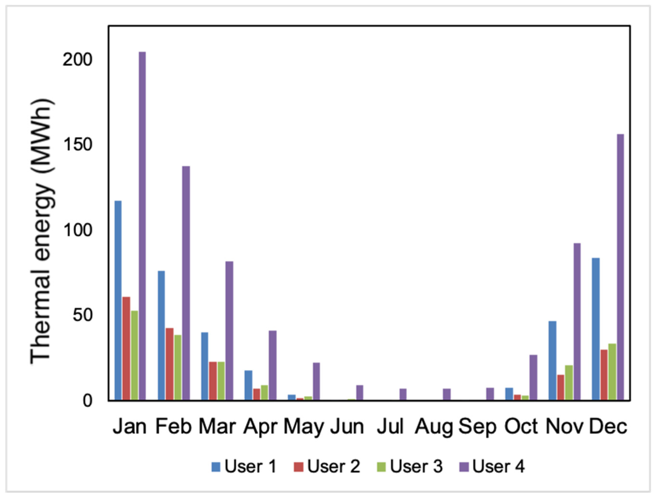
• Monthly consumptions were known from (approximately) weekly readings available at each user for the year 2019.
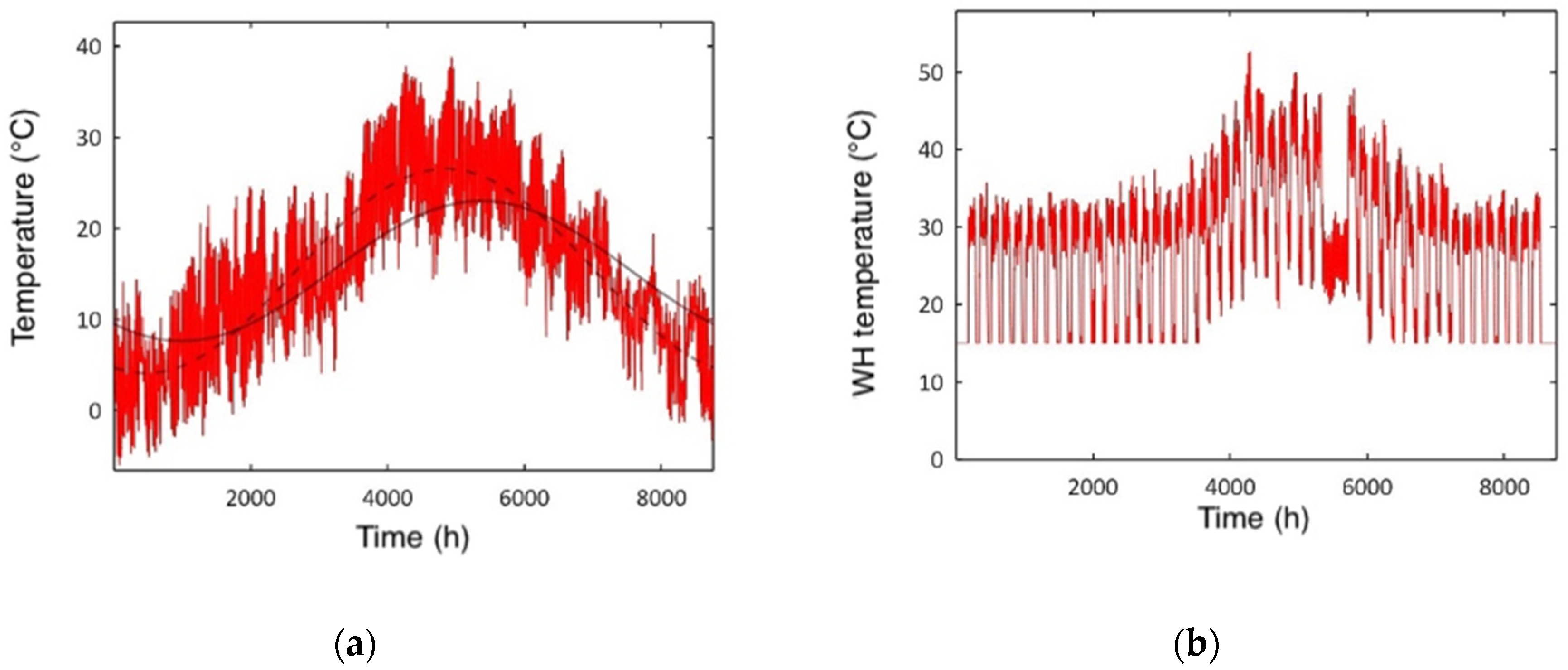
• Single-day consumptions were then estimated by distributing monthly consumptions proportionally to the heating degree days, which, in turn, were calculated from the ambient temperature data retrieved by a nearby weather station for the year 2019 (shown in Figure 4).
• Hourly consumptions were finally obtained by assuming fixed patterns for space heating (SH) and sanitary hot water (SHW), shown in the right panel of Figure 3. The SH pattern was built by averaging the available high-frequency data measured in a few winter days. Sanitary hot water (SWH) consumptions, assumed basically constant on a daily basis throughout the year, were estimated from summer weeks, with a random pattern in the interval 06:00–23:00.

One can recognise from the nonsymmetrical profile in the left panel of Figure 3 that the winter at the beginning of 2019 was colder than that at the end of 2019, as can be seen in the ambient temperature profile of Figure 4.

Besides the user load profiles, the models require as an input the temperature pro-files of the sources (in order to assign the network inlet temperature) and of the ground (in order to estimate the thermal losses).

The waste heat (WH) source is known to be typically available from Tuesday at 08:00 until Saturday at 16:00 (i.e., 62% of the week time), as it corresponds to a process that works on 3 shifts. This schedule is replicated every week, except for the two weeks of holidays both in the winter and in the summer (Christmas period and mid of August). The WH temperature fluctuates in a range of about 5 K around 30 °C, and, being related to the cooling towers, it is expected to be affected by the ambient temperature. On the basis of this information, the stochastic profile shown in Figure 4 was built. In the absence of further details, the temperature available on the network side was assumed to be 5 K less (i.e., 25 °C on average), with a rather conservative assumption on the heat exchanger performance.

The second source, operating when waste heat is not available, is provided by aquifer wells pumping ground water in an open loop from a depth of about 40 m. The supply temperature is mostly constant throughout the year and equal to 15 °C (corresponding to the average ambient temperature, as seasonal fluctuations do not affect the ground at this depth).

The temperature of the ground around pipes ($T_g$), which is important to calculate the network heat losses, was calculated according to a standard textbook formula [20,21,22] as a function of the time of the year and the depth below the ground surface, namely:

$$T_g\left(t\right)=T_{avg}-\Delta T_{amp} \exp \left(-z\sqrt{\frac{\pi }{t_{cyc} \alpha }}\right)\cos \left(\frac{2\pi }{t_{cyc}}\left(t-t_{min}\right)-z\sqrt{\frac{\pi }{t_{cyc} \alpha }}\right).$$

(1)

For $z$ = 0, which corresponds to ground surface, this equation is reduced to a simple sinusoidal function $T_{avg}+\Delta T_{amp}\cos \left[\left(t-t_{min}\right)2\pi /t_{cyc}\right]$. Here, the cycle period $t_{cyc}$ is assumed to be one year (daily oscillations are neglected), and hence, parameter $T_{avg}$ must be set equal to the yearly average ambient temperature. Moreover, the parameters $\Delta T_{amp}$ and $t_{min}$ can be identified by fitting the sinusoidal function to the ambient temperature data. The latter were retrieved by a local weather station and are reported as a red line in Figure 4a. The resulting curve for $z$ = 0 is represented by a black dashed line in Figure 4a, where the semi-amplitude of the oscillation corresponds to $\Delta T_{amp}$ and the minimum occurs at time $t_{min}$. Whenever $z\ne 0$, an exponential decay factor and a delay term appear in Equation (1), both depending on the ground thermal diffusivity $\alpha$, which is here assumed to be 7 × 10⁻⁷ m²/s (22). The network pipes are at a depth of about 1 m and the corresponding calculated ground temperature is represented by the black solid line in Figure 4a, showing a difference of more than 10 degrees between winter and summer. One can recognize the smaller amplitude and the delay (depending on ground capacity) with respect to the approximated surface temperature. Due to the exponential term, oscillations quickly decrease with depth, converging towards $T_g\simeq T_{avg}$. It is worth noting that Equation (1) typically provides a reasonable description only for the initial ground layer (order of 20 m), while at higher depths other effects come into play.

The distribution temperature on the user side of the substations is also an important parameter, as it significantly affects the HP performance. Sanitary hot water is typically generated at 55 °C (small differences can occur among users), while space heating follows a climatic curve slightly different for each user. As an order of magnitude, the minimum supply temperature for SH is around 45 °C (used for ambient temperatures of about 7 °C or higher), while the maximum supply temperature is around 55 °C (used for ambient temperatures of about 2 °C or lower).

All user substations comprise multiple HPs in parallel. Depending on the load, a variable number of machines is in operation. This provides a more cost-effective modulation option with respect to a single large heat pump. All the installed HPs are provided by the same supplier, though two different sizes were chosen in order to better match the different users’ thermal needs (see, also, Figure 2). The data sheets of the two used machine versions exhibit very similar performances in term of the COP (coefficient of performance). Hence, in order to simplify the modelling, an average performance map was built using a COP function of the following kind [23]:

$$\mathrm{COP}={\eta }_m {\mathrm{COP}}_C+1-{\eta }_m,$$

(2)

where ${\mathrm{COP}}_C$ is the Carnot COP calculated from the condenser and evaporator temperatures of the refrigerant $T_c$ and $T_e$ (to be expressed in Kelvin), which in turn can be roughly related to the external fluid outlet temperatures by $T_c=T_{c,o}+\Delta T_{HEX}$ and $T_e=T_{e,o}-\Delta T_{HEX}$. Only two parameters are required by this COP function: the compressor efficiency ${\eta }_m$, typically of the order of 50–60%, and the heat exchanger temperature lift $\Delta T_{HEX}$ (assumed to be the same for condenser and evaporator), typically of the order of 2 K. For the HPs installed at Ospitaletto, fitting this function on the machine data sheets yielded ${\eta }_m$ = 53% and $\Delta T_{HEX}$ = 2.15 K. With these parameters and for the operating conditions of interest, the discrepancy between the above formula and the data sheet values is in the range 5–15%. While more accurate HP performance maps can be used, this function has the benefit of providing a simple physical understanding of the effects related to variations in operating temperatures with a minimum number of parameters.

Concerning the above model inputs, it is worth pointing out that a detailed model also requires specific inputs in order to deliver its potential. The analysis of single users requires information on their individual profiles. In the absence of detailed data, various solutions to build input profiles exist in the literature (e.g., the use of specific consumption estimates coupled to building floor areas and heating degree day profiles), with different impacts on the resulting accuracy.

2.2. The Models

This section provides a description of the approximate and detailed models.

2.2.1. Approximate Model

The original version of this model was developed as an Excel tool during the FLEXYNETS project, with the specific aim of analysing neutral-temperature networks with decentralised HPs (though the analysis of conventional networks was also possible). The model can be downloaded at the FLEXYNETS website [8], along with a guide that includes a detailed description. The model concept is based on a lumped parameter approach: all network users are considered as a single aggregated load. Moreover, a time-slicing implementation is used for all profiles, using a single representative day for each month. These choices allow for very short execution times, making the model suitable for scenario analysis (e.g., in parametric or optimisation studies). In order to minimise user inputs, the tool offers many predefined options, though they can be customised. For the case considered here, the following inputs were explicitly provided:

• Monthly heat consumptions of aggregated users.
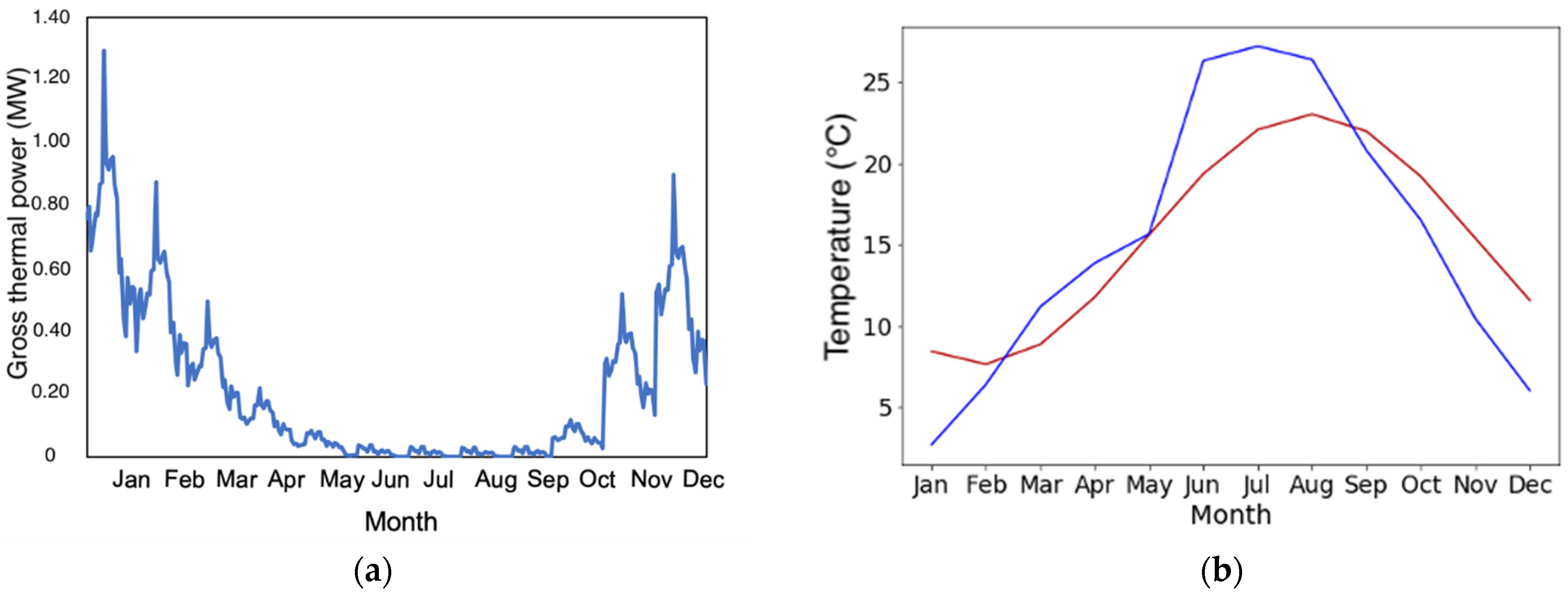
• Monthly average ambient temperature profile.
• Source temperatures. A constant supply temperature of 21.2 °C was set as a weighted average between the waste heat temperature of 25 °C (available for about 62% of the time) and the aquifer well temperature of 15 °C (available for the remaining time).
• User temperatures. An average climatic curve was set according to the description in the previous section.
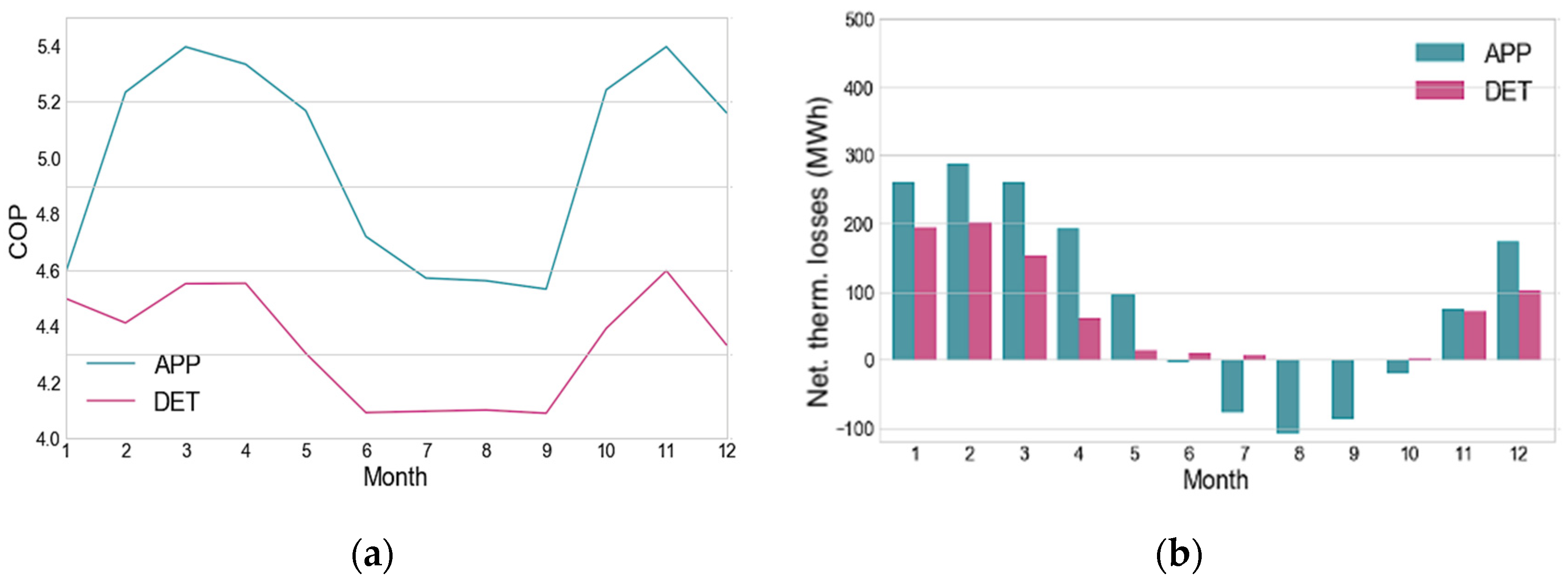
• HP performance. The above COP function calibrated on the available data sheets was used.
• Network. By default, the model estimates the network main parameters (lengths, distribution of pipe diameters, heat exchange coefficients, etc.) based on the overall heat demand and assuming typical building densities and pipe sizes. In this case, however, the geometry of Figure 1 was used to obtain the correct pipe distribution and heat exchange coefficients (see below).

In this model, the aggregated thermal load of all users is shown in Figure 5 (with a pattern of 24 h for each month). This profile was estimated as follows:

• Monthly consumptions were known from (approximately) weekly readings available at each user for the year 2019.
• Monthly consumptions were then evenly distributed according to the corresponding number of days to estimate the consumption of a single reference day for each month.
• Hourly loads were obtained by assuming fixed patterns for space heating (SH) and sanitary hot water (SHW), shown in the right panel of Figure 3. Consequently, the annual analysis consists of 24 h × 12 = 288 h.

The ground temperature ($T_g$) was estimated according to Equation (1) but applied on a monthly basis, i.e., a single temperature was calculated for each reference day ($t=15+\left[\mathrm{M}-1\right]\times 30, \mathrm{M}=1, \dots , 12$, and $t_{cyc}=365$; using days as the time unit, the ground thermal diffusivity becomes $\alpha =0.068$ m²/day). The resulting monthly values for the ambient and ground temperatures are presented on the right panel of Figure 5.

The seasonal amplitude variation decreases with the depth; in fact, below 12 m, the ground temperature is almost constant. It was then assumed that the extracted water from the aquifer wells reached a constant temperature at a depth of 40 m.

The overall thermal losses on the supply ($E_{loss,s}$) and return ($E_{loss,r}$) pipes were estimated as a function of the following network characteristics: pipes lengths and diameters, pipe insulation properties given by an average overall heat exchange coefficient ($U_{avg}$), network supply ($T_{net,s}$) and return temperatures ($T_{net,r}$), and ground temperature ($T_g$). The supply return network temperature was assumed to be at a constant 5-K difference, according to the expected HP evaporator operation:

$$E_{loss,s}=U_{avg}\times \left(T_{net,s}-T_g\right),$$

(3)

$$E_{loss,r}=U_{avg}\times \left(T_{net,r}-T_g\right),$$

(4)

$$U_{avg}={\displaystyle \sum }_{i=1}^n{\displaystyle \sum }_{j=1}^m{U}_{pip{e}_{i,j}}\times L_{pip{e}_{i,j}},$$

(5)

where $U_{pip{e}_{i,j}}=$ the pipe heat exchange coefficient of diameter i and material j, and $L_{pip{e}_{i,j}}=$ the overall lengths of the pipes with diameter i and material j.

As the network geometry and pipes characteristics were known, all the material properties were obtained from data sheets.

The model also includes economic inputs (e.g., investment costs, energy prices and interest rates), which are, however, not discussed here.

The model main outputs provide:

• HP electricity consumptions
• Thermal energy delivered by the network (on the evaporator side of the HPs)
• Thermal losses
• Pumping consumptions
• CO₂ emissions

Similar to the economic inputs, the economic outputs provided by the tool, which are based on the annuity method, are not discussed in this work.

For this analysis, several default options of the original model were modified according to the input list provided above. Moreover, the COP function and the formula for pumping consumptions were updated. A discussion of possible improvements to the tool that would increase its flexibility is reported below.

2.2.2. Detailed Model

The detailed model used here was developed within the LIFE4HeatRecovery pro-ject. It is coded in Octave (preserving compatibility with MATLAB), and it describes the hydraulic and thermal dynamics of the network. The network geometry is implemented as a graph, with vertices positioned according to Figure 1. The hydraulic boundary conditions are provided by flow rates at user vertices (that are calculated from the user load profiles assuming a constant supply return temperature difference of 5 °C, controlled by regulating valves at HP substations) and by the pressure at a reference vertex. The thermal boundary conditions are provided by source temperatures. The hydraulic part is solved independently from the thermal part by using the Kirchhoff laws at network nodes [24]. The relation between the pressure losses $\Delta p$ and flow rate $\dot{V}$ is assumed to be of the type

$$\Delta p\propto {\dot{V}}^n,$$

(6)

while pump control basically assumes a fixed pressure difference. The solution of the thermal part depends instead on the hydraulic solution, as it uses a one-dimensional heat transfer equation which depends on velocity (and neglects thermal diffusion) [25].

$$\left({\partial }_t+v{\partial }_x\right) T_f=-\frac{T_f-T_g}{\tau },$$

(7)

where $T_f$ is the fluid temperature, $T_g$ is the ground temperature around the pipes (see Equation (1)), $v$ is the fluid velocity, and $\tau$ is a time constant. The latter is related to the overall pipe heat loss coefficient $U_{avg}$ (which can be found in pipe data sheets or can be calculated with standard formulas on the basis of pipe geometric data and material thermal conductivities) by $\tau =\rho c_p \pi {\left(D/2\right)}^2/U_{avg}$, where $D$ is the pipe diameter and $\rho$ and $c_p$ are respectively the water density and specific heat. For the case of constant ground temperature, solution of Equation (7) can be written as

$$T_f\left(t,x\right)=T_g+[T_f(t_0,x-{\int }_{t_0}^{t}v\left(t^{\prime }\right) d{t}^{\prime })-T_g]e^{-\left(t-t_0\right)/\tau },$$

(8)

where $t_0$ is some initial time. Exploiting this semi-analytical solution, the outlet temperature of a pipe section can be calculated as a function of the inlet temperature at previous times. In practice, this was implemented by coding in Matlab the analogous of the Modelica spatialDistribution() function [26]. The solution could be generalized to non-constant ground temperature, however, this effect was neglected since the time-scale for its variations is much longer than that for the network operation. With this assumption, the validity of solution (8) for Equation (8) can be checked by explicitly carrying out the time and space derivatives.

The main inputs of the detailed model correspond to the list provided for the approximate model, though they, of course, need to be more detailed. In particular:

• A load profile for each single user needs to be provided. Since the HPs of all the users come from the same supplier, the single COP function reported in Equation (2) was used.
• All profiles are included as full hourly profiles.

Indeed, while the detailed model can, in principle, be run with any time step, for this analysis, simulations were carried out with an hourly time step for a full year (i.e., 24 h × 365 = 8760 h). The flow rates, pressures and temperatures are available at each vertex at any time step.

2.2.3. Key Performance Indicators and Input Parameters

It is possible to get the key performance indicators (KPI) used for the comparison of both models integrating energies on an annual basis. The energy delivered on the HP condenser side ($E_{th,HP,c}$), assuming an adiabatic system, is the sum between the HP electric consumptions ($E_{el,HP}$) and the heat absorbed on the evaporator (i.e., network) side ($E_{th,HP, e}$). The total heat lost along the distribution network ($E_{th,loss}$) is assessed through Equations (3) and (4). In addition, the seasonal COP (SCOP) is calculated as the ratio between the annual thermal energy on the condenser side and the yearly electric energy ($\mathrm{SCOP}=E_{th,HP,c}/E_{el,HP}$).

Besides the yearly analysis, it is also of interest to assess these indicators on a monthly basis to evaluate seasonality effects. The monthly COP is defined as the ratio between the thermal energy at the condenser and the electric energy both calculated for the given month.

The COP function used in the two models is the same; however, the network-side and user-side temperatures are different: (i) for the network-side temperature, the approximate model uses a constant temperature given by the weighted average of the source temperatures, while the detailed model uses the temperature derived from the propagation of the time-dependent source temperatures along the pipes (taking into account all thermal losses); (ii) for the user-side temperature, the approximate model uses an average climatic curve, while the detailed model uses the actual climatic curves of the single users.

In

Table 1. Common input parameters used in each model.

Parameters	Approximate Model	Detailed Model
$T_{avg}$	15.3 °C	15.3 °C
$\Delta T_{amp}$	16.9 K	16.9 K
$\alpha$	0.068 m2/day	7 × 10−7 m2/s
$t_{cyc}$	365 days	8760 h
$t_{min}$	30th day	Hour 720
$z_{net}$	1 m	1 m
$z_{aq}$	40 m	40 m
${\eta }_m$	53%	53%
$\Delta T_{HEX}$	2.15 K	2.15 K
$T_{net,s}$	21.2 °C	Equation (8)
$T_{net,r}$	16.2 °C	Equation (8)

, it is shown the input data used in each model. The main differences are due to the different time resolutions.

3. Results and Discussion

The aforementioned models were compared in a case study. While true model validations involving comparisons with real data are planned for future works, this cross-verification already allows for the assessment of the impacts of some of the considered approximations.

The comparisons can only be carried out on the aggregated values and at a monthly level, given that these are the spatial and temporary scales of the approximate model. The overall thermal consumptions on the user side are clearly the same for both models, as these are inputs. However, differences can be expected in the over-all electric consumptions of the HPs (due to different detail levels in the calculations of the network and user temperatures) and, consequently, on the network heat flows. Moreover, significant differences could exist for thermal losses and pumping consumptions, given the very simplified assumptions used in the approximate model.

As mentioned above, the detailed model yields the values of the different operating variables at each network vertex. For this analysis, vertices were included for each little node shown in Figure 1, where some geometric change occurs (pipe bends or changes in pipe types). Correspondingly, values at all these vertices are available. As an example, Figure 6 shows the behaviour of flow rate (left panel) and temperature (right panel) for the supply (red lines) and return (blue lines) pipes across the path connecting source $s_1$ and the most distant user $u_4$. The plots refer to the peak hour of a typical winter day. It can be observed that the flow rate remains constant up to a distance of about 1250 m, where there is a drop since part of the flow is diverted towards user $u_1$. At the next vertex the flow drops again, as part of the flow goes to the branch corresponding to users $u_2$ and $u_3$. The return flow of course is identical to the supply flow, but with an opposite sign. As regards the temperature plot, one can recognize a temperature drop due to thermal losses. The slope of the curve is not constant: this is due to the different pipe types used in the network. Up to a distance of about 1200 m the curve slope is higher, yielding a drop of about 1.2 °C: this part of the network is built with non-insulated PN10 HDPE pipes, with an overall heat loss coefficient $U_{avg}$ = 18.7 W/(m⋅K). In the final part of the network, instead, mainly pre-insulated steel pipes are used, where $U$ = 0.43 W/(m⋅K). It is easy to check the order of magnitudes of the corresponding losses: given that the difference between the fluid temperature and the ground temperature in winter is of the order of 15 °C, for a distance of 1000 m the loss power for HDPE pipes would be about 280 kW (supply only). In terms of temperature drop, for the flow rate of 0.033 m³/s shown in Figure 6, this power would correspond to about 2 °C. For pre-insulated steel pipes, the loss would instead be about 6.45 kW, with a negligible temperature variation.

Electric and evaporator energies for the HPs are shown in Figure 7. These are crucial quantities for this type of networks, where the operating consumptions of HPs provide a major contribution to costs and carbon emissions (through electricity). One can see that the two models are in reasonable agreement.

The monthly average COP is reported on the left panel of Figure 8. One can see that the approximate model estimates a higher COP than the detailed model. This is mainly due to the higher temperature assumed on the evaporator side.

Concerning thermal losses, the predictions of the two models are reported in the right panel of Figure 8. The approximate estimate is typically higher than the detailed one. A major difference appears in the summer. Here, the approximate model estimates the presence of significant thermal gains, as the ground temperature can be higher than the network temperature, especially when waste heat is not available. The approximate model calculates the gains and losses on the basis of this temperature difference, regardless of the network operation. In the detailed model, losses and gains are calculated, taking into account the network operation; during the long summer periods without significant demand, in the detailed model, the network temperature reaches an equilibrium with the ground temperature, and no further heat exchange occurs. On the other hand, during the winter, the thermal losses predicted by the two models show similar values, showing that the general network structure assumed by the approximate model reasonably applies to this case. Similar conclusions can be reached on the basis of the pumping consumptions, where the predictions of the approximate model are about 50% higher than the detailed model.

Regarding the overall yearly performance of the network, one has the results reported in

Table 2. Yearly performances and energy balances for the two considered models. SCOP: seasonal coefficient of performance. arb. u.: arbitrary units.

Quantity	Unit	Approximate Model	Detailed Model
SCOP	arb. u.	5.0	4.5
$E_{th,HP,c}$	MWh/y	1558	1559
$E_{th,HP,e}$	MWh/y	1249	1206
$E_{el,HP}$	MWh/y	309	350
$E_{th,loss}$	MWh/y	1045	816
$E_{el,pump}$	MWh/y	38	20
CO2	t CO2/y	113	121

. Here, it is observed the SCOP, corresponding to the average HP COP, the yearly thermal energy supplied at the condenser side of the HPs ($E_{th,HP,c}$), corresponding to the user consumptions provided as an input, the yearly thermal energy at the evaporator side ($E_{th,HP,e}$), corresponding to the energy delivered by the network at user substations, the yearly electric energy consumed by HPs ($E_{el,HP}$), the network thermal losses ($E_{th,loss}$), the electricity consumptions for network pumping ($E_{el,pump}$), and, finally, the carbon emissions calculated from overall electric consumptions ($E_{el,HP}+E_{el,pump}$) multiplied by an emission factor of 0.327 t_CO2/MWh_el, estimated for the production mix of the Italian electric grid in Reference [27].

The results for the HP electric consumptions, heat absorbed by HPs from the network and average COP are, of course, strictly linked, and discrepancies between the two models can be explained with the different temperature values, as mentioned above. It is important to point out that, also, the detailed model currently neglects some effects; the substations are very simplified, and the transient effects in the operation of multiple HPs in parallel are not included.

The thermal losses results show the very strong impact of using non-insulated pipes, even at these low temperatures. According to the detailed model, about 40% of the heat injected into the network (by waste heat and aquifer wells) is lost in the ground (46%, according to the approximate model, where, however, a compensation between the gains and losses occurring at different months was taken into account). For the considered network, the waste heat is abundant and free; in such cases, the choice of non-insulated pipes can reduce investment costs without damaging the operating costs. In other cases, however, the choice of pre-insulated pipes (possibly with the smallest available thicknesses) might be more convenient.

The pumping consumptions were estimated to be relatively small by both models, in spite of the supply return temperature difference of only 5 °C. According to the detailed model, the electric energy needed for pumping is about 1.7% of the thermal energy delivered at the HP evaporators (or about 1.0% of the thermal energy injected at the sources), while, according to the approximate model, is almost twice as high. This is, of course, related to the sizing of the pipe diameters. The discrepancy between the two models is rather high in this case. In this respect, further improvements would be needed also for the detailed model, which is currently neglecting some losses (e.g., head losses at the pipe geometric changes), thereby probably underestimating the actual values.

As far as carbon emissions are concerned, in this case, the result directly follows from the electric consumption calculations. Indeed, this is the only source of non-renewable energy included in this type of network. Similarly, one can estimate the primary energy factor (PEF) of the network. Assuming a PEF = 2 for the Italian electric grid [28], the network PEF is estimated to be 0.48 by the detailed model and 0.45 by the approximate model. The strong difference between electricity consumptions for HPs and for pumping shows that, in order to properly estimate the sustainability of this type of district system, most attention should be devoted to the modelling of HPs and to the proper calculations of the network and user temperatures, in order to get the most possible accurate estimate for the COP.

Finally, it is useful to report about the numerical performances of the two approaches. While the execution of the approximate model is basically immediate, the detailed model requires about 30 min to solve the considered network (about 50 vertices) for a full year with hourly time steps on a standard laptop with a quad-core CPU. The solution time is mainly affected by the chosen implementation for the thermal calculations and by the chosen number of vertices (here, kept high in order to keep track of several small changes in the pipes and to show the analysis for a nontrivial geometry; several pipe sections could be merged if the computational speed was prioritised). This makes clear the different application of the two models: while intermediate approximations levels could be chosen, it would be impractical to use such a detailed model for parametric or optimisation tasks, where the model needs to be repeatedly solved for hundreds or thousands of times.

4. Conclusions

This paper discusses the modelling of an existing neutral-temperature network with decentralised heat pumps located in Ospitaletto, Italy. Both an approximate model (suitable for scenario analysis) and a detailed model (suitable for punctual analysis) were used, and the corresponding results for the monthly and yearly energy balances were compared. The two models were found to be in reasonable agreement: for the key quantity of the overall electricity consumptions, a difference of about 15% was observed. The main differences were identified in the values of the operating temperatures on the network and user sides affecting the heat pump operation. It is expected that a specific calibration of the parameters used in the approximate model (instead of using precalculated values) could further improve the agreement, although such a calibration would be most meaningful through real data and is, therefore, left for future works. From this point of view, for the simple network considered here, the structure of the approximate model seems suitable to obtain accurate outputs, though the best value of the aggregated parameters is difficult to be calculated a priori. This task could be devoted to the detailed model, while, once calibrated, the approximate model could be used to explore similar scenarios. On the other hand, it is not obvious that the aggregated approach is valid for more complex networks.

As regards the considered network, seasonal performance factors of 4.2 (detailed model) and 4.5 (approximate model) were estimated (including the heat pumps and network pumping), with primary energy factors lower than 0.5. This shows the environmental advantage of this type of network compared to individual boilers (where the primary energy factor is of the order of 1 or higher) and how, even in the absence of typical high-temperature sources used in district heating (like incinerators or combined heat and power), network solutions can be beneficial.

Several improvements to the presented models are planned for future works. In the approximate model, an hourly base analysis for the entire year could replace the time slicing, still preserving fast solution times. This would make the analysis easier for long-term storage effects not included here but interesting to be considered in the context of waste heat and renewable sources (which often have an availability profile that does not match the load profile). Moreover, the implementation of substations in both models could be made more accurate. A crucial step will, anyway, be the validation against real data planned within the LIFE4HeatRecovery project.

References

- Werner, S. District Heating and Cooling; Elsevier: Amsterdam, The Netherlands, 2013; Available online: http://urn.kb.se/resolve?urn=urn:nbn:se:hh:diva-24115 (accessed on 20 August 2020).
- FLEXYNETS Project (EU H2020, GA No. 649820). Available online: http://www.flexynets.eu (accessed on 7 August 2020).
- Lund, H.; Werner, S.; Wiltshire, R.; Svendsen, S.; Thorsen, J.E.; Hvelplund, F.; Mathiesen, B.V. 4th Generation District Heating (4GDH): Integrating smart thermal grids into future sustainable energy systems. Energy 2014, 68, 1–11. [Google Scholar] [CrossRef]
- Averfalk, H.; Werner, S. Economic benefits of fourth generation district heating. Energy 2020, 193, 116727. [Google Scholar] [CrossRef]
- Lund, H.; Østergaard, P.A.; Chang, M.; Werner, S.; Svendsen, S.; Sorknæs, P.; Thorsen, J.E.; Hvelplund, F.; Mortensen, B.O.G.; Mathiesen, B.V.; et al. The status of 4th generation district heating: Research and results. Energy 2018, 164, 147–159. [Google Scholar] [CrossRef]
- Østergaard, P.A.; Andersen, A.N. Booster heat pumps and central heat pumps in district heating. Appl. Energy 2016, 184, 1374–1388. [Google Scholar] [CrossRef]
- Østergaard, P.A.; Andersen, A.N. Economic feasibility of booster heat pumps in heat pump-based district heating systems. Energy 2018, 155, 921–929. [Google Scholar] [CrossRef]
- Buffa, S.; Cozzini, M.; D’Antoni, M.; Baratieri, M.; Fedrizzi, R. 5th generation district heating and cooling systems: A review of existing cases in Europe. Renew. Sustain. Energy Rev. 2019, 104, 504–522. [Google Scholar] [CrossRef]
- Wirtz, M.; Kivilip, L.; Remmen, P.; Müller, D. 5th Generation District Heating: A novel design approach based on mathematical optimization. Appl. Energy 2020, 260, 114158. [Google Scholar] [CrossRef]
- von Rhein, J.; Henze, G.P.; Long, N.; Fu, Y. Development of a topology analysis tool for fifth-generation district heating and cooling networks. Energy Convers. Manag. 2019, 196, 705–716. [Google Scholar] [CrossRef]
- Life4heatrecovery Project. Available online: http://www.life4heatrecovery.eu/en/ (accessed on 29 September 2020).
- Ma, W.; Fang, S.; Liu, G.; Zhou, R. Modeling of district load forecasting for distributed energy system. Appl. Energy 2017, 204, 181–205. [Google Scholar] [CrossRef]
- Termis Engineering|Schneider Electric. Available online: https://www.se.com/my/en/product-range-presentation/61613-termis-engineering/ (accessed on 16 November 2020).
- Comsof Heat-District Heating Network Planning & Design Software. Available online: https://comsof.com/heat/ (accessed on 16 November 2020).
- THERMOS Tool. THERMOS. 2020. Available online: https://www.thermos-project.eu/thermos-tool/thermos-tool/ (accessed on 16 November 2020).
- The PLANHEAT Tool. Planheat. Available online: https://planheat.eu/the-planheat-tool/ (accessed on 16 November 2020).
- EnergyPLAN. Available online: https://www.energyplan.eu/ (accessed on 16 November 2020).
- LEAP. Available online: https://leap.sei.org/default.asp (accessed on 16 November 2020).
- Cozzini, M.; D’Antoni, M.; Buffa, S.; Fedrizzi, R.; Bava, F. District Heating and Cooling Networks Based on Decentralized Heat Pumps: Energy Efficiency and Reversibility at Affordable Costs. HPT Mag 2018, 36, 25–29. [Google Scholar]
- Eckert, E.; Drake, R.M. Heat and Mass Transfer; McGraw-Hill Inc.: New York, NY, USA, 1959. [Google Scholar]
- Jaeger, J.C.; Carslaw, H.S. Conduction of Heat in Solids; Oxford University Press: Oxford, UK, 1959. [Google Scholar]
- Banks, D. An Introduction to Thermogeology: Ground Source Heating and Cooling; John Wiley & Sons: Hoboken, NJ, USA, 2012. [Google Scholar]
- Grassi, W. Heat Pumps: Fundamentals and Applications; Springer: Berlin/Heidelberg, Germany, 2018. [Google Scholar]
- Ben Hassine, I.; Eicker, U. Impact of load structure variation and solar thermal energy integration on an existing district heating network. Appl. Therm. Eng. 2013, 50, 1437–1446. [Google Scholar] [CrossRef]
- Velut, S.; Tummescheit, H. Implementation of a transmission line model for fast simulation of fluid flow dynamics. In Proceedings of the 8th International Modelica Conference, Technical Univeristy, Dresden, Germany, 20–22 March 2011; Linköping University Electronic Press: Linköping, Sweden, 2011; pp. 446–453. [Google Scholar]
- Van der Heijde, B.; Fuchs, M.; Tugores, C.R.; Schweiger, G.; Sartor, K.; Basciotti, D.; Müller, D.; Nytsch-Geusen, C.; Wetter, M.; Helsen, L. Dynamic equation-based thermo-hydraulic pipe model for district heating and cooling systems. Energy Convers. Manag. 2017, 151, 158–169. [Google Scholar] [CrossRef] [Green Version]
- European Residual Mix|AIB. Available online: https://www.aib-net.org/facts/european-residual-mix (accessed on 6 November 2020).
- Noussan, M.; Roberto, R.; Nastasi, B. Performance Indicators of Electricity Generation at Country Level—The Case of Italy. Energies 2018, 11, 650. [Google Scholar] [CrossRef] [Green Version]