
Time-Dependent Upper Limits to the Performance of Large Wind Farms Due to Mesoscale Atmospheric Response


Abstract
:1. Introduction
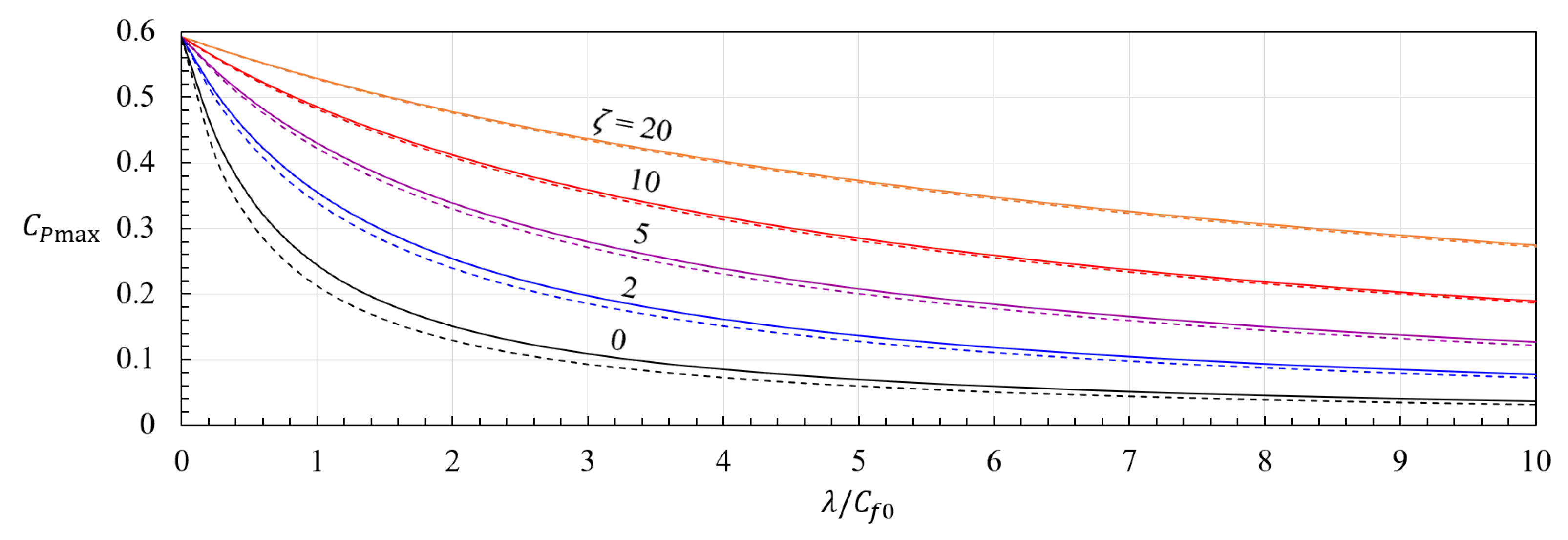
2. Theory
3. Methodology
3.1. Setup of NWP Simulations
3.2. How to Compute , and
4. Results
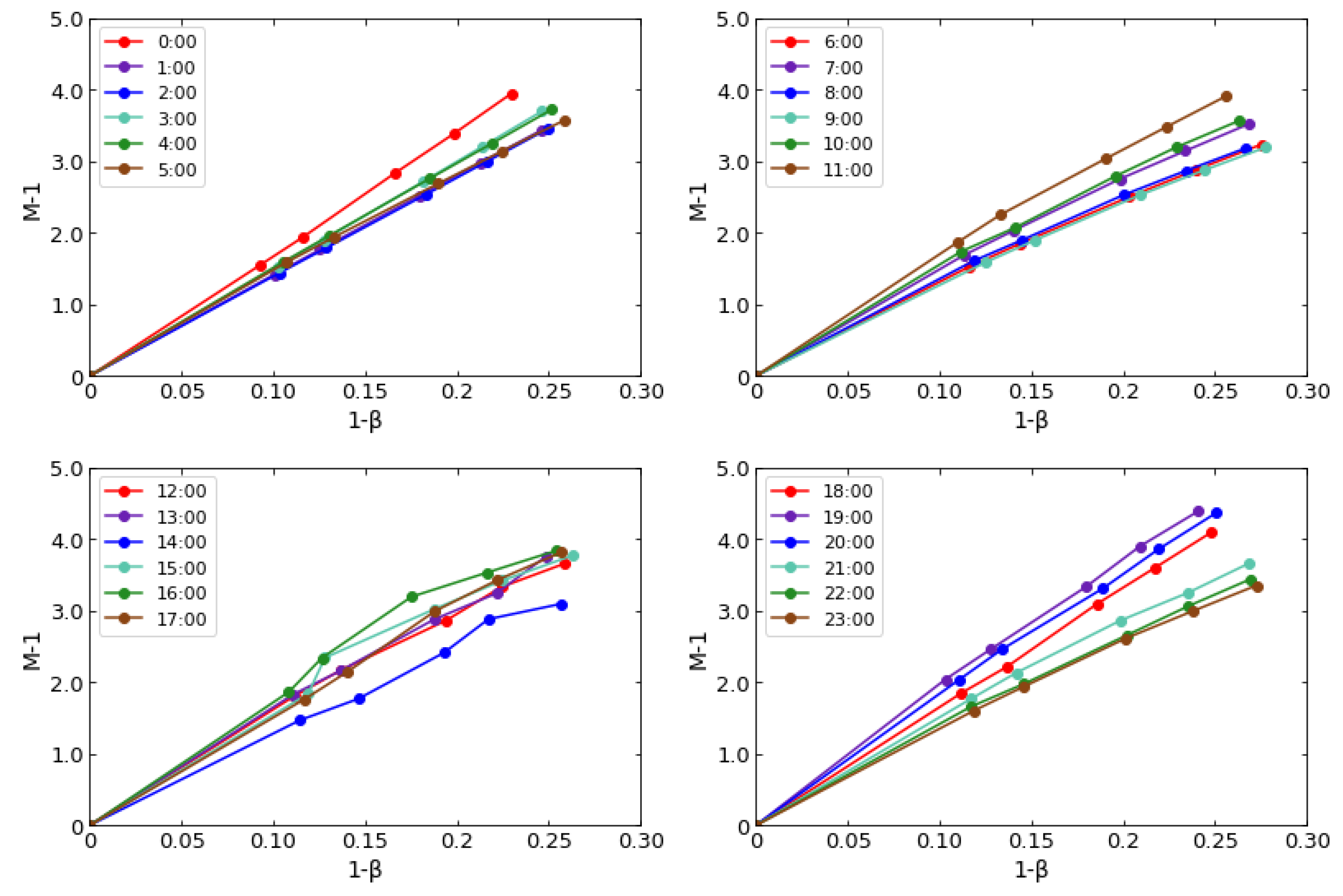
4.1. Linearity of the Atmospheric Response
4.2. Histogram of the Response Parameter
4.3. Time-Dependent Upper Limits to the Power Density
5. Discussion and Conclusions
Author Contributions
Funding
Institutional Review Board Statement
Informed Consent Statement
Data Availability Statement
Acknowledgments
Conflicts of Interest
Abbreviations
| ABL | Atmospheric boundary layer |
| AEP | Annual energy production |
| CFD | Computational fluid dynamics |
| NWP | Numerical weather prediction |
| RANS | Reynolds-averaged Navier–Stokes |
| UM | Unified Model |
References
- BEIS. Wind Powered Electricity in the UK. Available online: https://assets.publishing.service.gov.uk/government/uploads/system/uploads/attachment_data/file/875384/Wind_powered_electricity_in_the_UK.pdf (accessed on 6 October 2021).
- Bleeg, J.; Purcell, M.; Ruisi, R.; Traiger, E. Wind farm blockage and the consequences of neglecting its impact on energy production. Energies 2018, 11, 1609. [Google Scholar] [CrossRef] [Green Version]
- Ørsted. Ørsted Presents Update on Its Long-Term Financial Targets. Available online: https://orsted.com/en/company-announcement-list/2019/10/1937002 (accessed on 6 October 2021).
- Branlard, E.; Quon, E.; Forsting, A.R.M.; King, J.; Moriarty, P. Wind farm blockage effects: Comparison of different engineering models. J. Phys. Conf. Ser. 2020, 1618, 062036. [Google Scholar] [CrossRef]
- Segalini, A. An analytical model of wind-farm blockage. J. Renew. Sustain. Energy 2021, 13, 033307. [Google Scholar] [CrossRef]
- Nishino, T.; Dunstan, T.D. Two-scale momentum theory for time-dependent modelling of large wind farms. J. Fluid Mech. 2020, 894, A2. [Google Scholar] [CrossRef]
- Miller, L.M.; Brunsell, N.A.; Mechem, D.B.; Gans, F.; Monaghan, A.J.; Vautard, R.; Keith, D.W.; Kleidon, A. Two methods for estimating limits to large-scale wind power generation. Proc. Natl. Acad. Sci. USA 2015, 112, 11169–11174. [Google Scholar] [CrossRef] [PubMed] [Green Version]
- Fitch, A.C.; Olson, J.B.; Lundquist, J.K. Parameterization of Wind Farms in Climate Models. J. Clim. 2013, 26, 6439–6458. [Google Scholar] [CrossRef]
- Jacobson, M.Z.; Archer, C.L. Saturation wind power potential and its implications for wind energy. Proc. Natl. Acad. Sci. USA 2012, 109, 15679–15684. [Google Scholar] [CrossRef] [PubMed] [Green Version]
- Adams, A.S.; Keith, D.W. Are global wind power resource estimates overstated? Environ. Res. Lett. 2013, 8, 015021. [Google Scholar] [CrossRef]
- Borrman, R.; Rehfeldt, K.; Wallasch, A.K.; Lüers, S. Capacity Densities of European Offshore Wind Farms; Technical Report; Deutsche WindGuard GmbH: Hamburg, Germany, 2018. [Google Scholar]
- Enevoldsen, P.; Jacobson, M.Z. Data investigation of installed and output power densities of onshore and offshore wind turbines worldwide. Energy Sustain. Dev. 2021, 60, 40–51. [Google Scholar] [CrossRef]
- Nishino, T. Two-scale momentum theory for very large wind farms. J. Phys. Conf. Ser. 2016, 753, 032054. [Google Scholar] [CrossRef]
- Zapata, A.; Nishino, T.; Delafin, P.L. Theoretically optimal turbine resistance in very large wind farms. J. Phys. Conf. Ser. 2017, 854, 012051. [Google Scholar] [CrossRef] [Green Version]
- West, J.R.; Lele, S.K. Wind turbine performance in very large wind farms: Betz analysis revisited. Energies 2020, 13, 1078. [Google Scholar] [CrossRef] [Green Version]
- Nishino, T.; Hunter, W. Tuning turbine rotor design for very large wind farms. Proc. R. Soc. A 2018, 474, 20180237. [Google Scholar] [CrossRef] [Green Version]
- Walters, D.; Boutle, I.; Brooks, M.; Melvin, T.; Stratton, R.; Vosper, S.; Wells, H.; Williams, K.; Wood, N.; Allen, T.; et al. The Met Office Unified Model Global Atmosphere 6.0/6.1 and JULES Global Land 6.0/6.1 configurations. Geosci. Model Dev. 2017, 10, 1487–1520. [Google Scholar] [CrossRef] [Green Version]
- Bush, M.; Allen, T.; Bain, C.; Boutle, I.; Edwards, J.; Finnenkoetter, A.; Franklin, C.; Hanley, K.; Lean, H.; Lock, A.; et al. The first Met Office Unified Model–JULES Regional Atmosphere and Land configuration, RAL1. Geosci. Model Dev. 2020, 13, 1999–2029. [Google Scholar] [CrossRef] [Green Version]
- Lock, A.; Edwards, J.; Boutle, I. Unified Model Documentation Paper 024: The Parametrization of Boundary Layer Processes; Met Office: Exeter, UK, 2018. [Google Scholar]
- Archer, C.L.; Wu, S.; Ma, Y.; Jiménez, P.A. Two corrections for turbulent kinetic energy generated by wind farms in the WRF model. Mon. Weather. Rev. 2020, 148, 4823–4835. [Google Scholar] [CrossRef]
- Antonini, E.G.A.; Caldeira, K. Spatial constraints in large-scale expansion of wind power plants. Proc. Natl. Acad. Sci. USA 2021, 118, e2103875118. [Google Scholar] [CrossRef] [PubMed]
- Dunstan, T.; Murai, T.; Nishino, T. Validation of a theoretical model for large turbine array performance under realistic atmospheric conditions. In Proceedings of the AMS 23rd Symposium on Boundary Layers and Turbulence, Oklahoma City, OK, USA, 11–15 June 2018; p. 13A.3. [Google Scholar]
- Ma, L.; Dunstan, T.D.; Nishino, T. Analysing momentum balance over a large wind farm using a numerical weather prediction model. J. Phys. Conf. Ser. 2020, 1618, 062010. [Google Scholar] [CrossRef]
- Calaf, M.; Meneveau, C.; Meyers, J. Large eddy simulation study of fully developed wind-turbine array boundary layers. Phys. Fluids 2010, 22, 015110. [Google Scholar] [CrossRef] [Green Version]
- Nishino, T. Generalisation of the two-scale momentum theory for coupled wind turbine/farm optimisation. In Proceedings of the 25th National Symposium on Wind Engineering, Tokyo, Japan, 3–5 December 2018; pp. 97–102. [Google Scholar] [CrossRef]


| Parameter | Definition |
|---|---|
| Array density | |
| Average local thrust coefficient | |
| Bottom friction exponent | |
| Farm wind speed reduction factor | |
| Momentum availability factor | |
| Natural bottom friction coefficient |
| Parameter | Definition | Note |
|---|---|---|
| Array density | Input parameter | |
| Bottom friction exponent | Empirical (1.5–2.0) | |
| Farm wind speed reduction factor | Output parameter | |
| Local wind speed reduction factor | Input parameter | |
| Momentum response parameter | Obtained from NWP | |
| Natural bottom friction coefficient | Obtained from NWP |
| All Data Points | Only for | Only for m/s | |
|---|---|---|---|
| No. of points | 240 | 230 | 213 |
| Max | 49.3 | 23.9 | 23.6 |
| Min | −321 | 6.0 | −39.1 |
| Mean | 12.7 | 14.3 | 13.7 |
| Median | 13.6 | 13.8 | 13.5 |
| Std Dev | 22.6 | 3.6 | 5.1 |
Publisher’s Note: MDPI stays neutral with regard to jurisdictional claims in published maps and institutional affiliations. |
© 2021 by the authors. Licensee MDPI, Basel, Switzerland. This article is an open access article distributed under the terms and conditions of the Creative Commons Attribution (CC BY) license (https://creativecommons.org/licenses/by/4.0/).
Share and Cite
Patel, K.; Dunstan, T.D.; Nishino, T. Time-Dependent Upper Limits to the Performance of Large Wind Farms Due to Mesoscale Atmospheric Response. Energies 2021, 14, 6437. https://doi.org/10.3390/en14196437
Patel K, Dunstan TD, Nishino T. Time-Dependent Upper Limits to the Performance of Large Wind Farms Due to Mesoscale Atmospheric Response. Energies. 2021; 14(19):6437. https://doi.org/10.3390/en14196437
Chicago/Turabian StylePatel, Kelan, Thomas D. Dunstan, and Takafumi Nishino. 2021. "Time-Dependent Upper Limits to the Performance of Large Wind Farms Due to Mesoscale Atmospheric Response" Energies 14, no. 19: 6437. https://doi.org/10.3390/en14196437