Article

Analysis of Performance of Cavitation Models with Analytically Calculated Coefficients

Department of Engineering and Architecture, University of Trieste, Via Alfonso Valerio, 6/1, 34127 Trieste, Italy
*
Author to whom correspondence should be addressed.
Energies 2021, 14(19), 6425; https://doi.org/10.3390/en14196425
Submission received: 4 August 2021 / Revised: 23 September 2021 / Accepted: 29 September 2021 / Published: 8 October 2021

Abstract

:
Cavitation is often simulated using a mixture model, which considers the transport of an active scalar, namely the vapor fraction α v . Source and sink terms of the transport equation of α v , namely vaporization and condensation terms, rule the dynamics of the cavity and are described through different models. These models contain empirical coefficients generally calibrated through optimization processes. The purpose of this paper is to propose an analytical approach for the calculation of the coefficients, based on the time scales of vaporization and condensation processes. Four different models are compared considering as a test-case a two-dimensional flow around a cylinder. Some relevant quantities are analyzed both for standard value of coefficients, as found in the literature, and the coefficients calculated through the analytical approach. The study shows that the analytical computation of the coefficients of the model substantially improve the results, and the models considered give similar results, both in terms of cavitation regime and mean vapor fraction produced.

1. Introduction

Cavitation is a complex phenomenon, occurring in several engineering devices when flow pressure drops below the vapor pressure. Its own importance in naval and hydraulic engineering is confirmed by growing numerical and experimental studies, aimed at understanding and reproducing a multiphase process that involves different temporal and spatial scales. Examples of devices which may undergo cavitation are pressure pipes, especially near fittings or corners, or near bottlenecks, where the flow accelerates, or in the presence of a water hammer; cavitation is also common in hydraulic turbines and pumps and, also, it may affect ship propellers, due to low pressure occurring above the blades and in the presence of tip-vortex structures. Vapor phase formation generally affects the device performance, and bubble inception is found to produce intense noise and may damage solid surfaces. Once vapor is formed, it is transported by the flow through regions where pressure re-establishes above the vapor pressure, thus producing condensation and bubble implosion. This phase is of fundamental importance as well as the cavitation inception; for this reason many theoretical and experimental studies focused on these two aspects, considering the dynamics of a single bubble (see, among the others [1,2,3]). The implosion of vapor bubbles is a non-linear process and produces large pressure peaks (of the order of a hundred bars) in localized areas and micro-jets with velocity of the order of hundreds meters per second [4]; these phenomena cause high frequency pressure perturbations and micro-fractures on nearby structures [5], which are usually the blades of the propellers or pump impellers, and they can lead, over time, to deterioration or even collapse of the device. Furthermore, the high level of broad-band noise associated with cavitation is an important issue which is gaining increasing attention, mostly for cruise ships which need to minimize the noise for passengers welfare or to enter in protected areas [6].
Several numerical approaches were developed to treat cavitating flows, each of them suitable for the specific application and cavitation regime considered, e.g., homogeneous cavitation, sheet cavitation or bubbly flows. Among others, the Eulerian front-tracking techniques [7], and the Euler-Lagrangian methods [8], suitable for small-scale processes, where a countable number of bubbles is present. More recently, the Eulerian-Lagrangian method has been improved to treat multiscale processes characterized by the simultaneous presence of bubbles and sheet cavitation (see the very recent paper [9]). For engineering applications, homogeneous mixture methods are commonly employed, due to their practicality and adaptability to large-scale cavitation cases. In these methods, the phases (liquid, vapor, and possibly gas) are treated through the use of a scalar field α , indicating the phase fraction, and they may be divided into two main categories: (i) barotropic models, where a state equation is adopted as closing relation between the vapor/gas fraction and the pressure (among other we refer to Dellannoy and Kueny [10], Rebound et al. [11], Song and He [12], Coutier-Delgosha et al. [13] and Qin et al. [14]); (ii) transport equation models, where the phase fraction is governed by a non-linear partial differential equation, whose form varies according to the model considered.
The latter relies on two source/sink terms, which are needed to model the phenomena of vaporization and condensation: several models have been developed to parametrize these processes as function of resolved variables; among them, we mention: the Merkle et al. [15] model in which the source terms are related to the density variation, proportional to the dynamic pressure; the Kunz et al. [16] model uses the same vaporization source term as Merkle’s model and a simplified Ginzburg-Landau potential for the condensation one; Senocak and Shyy [17] used the mass-momentum conservation equation at the interface to evaluate the source terms as a function of known flow variables. Singhal et al. [18], Zwart et al. [19], and Schnerr and Sauer 2001 [20] based the source terms on the simplification of the Rayleigh-Plesset equation for the dynamic of a bubble; Saito et al. [21] evaluated the source terms based on the theory of evaporation and condensation on a plane surface.
An important issue related to these models is the use of empirical coefficients, which are needed since the terms describing the condensation/vaporization processes are simplified version of complex physical relationship (the most indicative is perhaps the Schnerr-Sauer model, which considers only the terms of the Rayleigh-Plesset equation related to the asymptotic growth of bubbles). The condensation/vaporization coefficients C c and C v may be calibrated for the study of the specific problem such as the flow around a hydrofoil [22] or a marine propeller [23]; usually calibration of the coefficients is performed using optimization techniques [24], where the values of the coefficients are evaluated forcing the solution to obtain optimal values of some mean quantities, such as the pressure coefficient or thrust and torque coefficients, the latter in case of marine propellers.
In the present study, we propose a new procedure for the calculation of the coefficients C c and C v , which, actually, act as accelerators/decelerators of the vaporization and condensation processes. We consider four models (Merkle, Schnerr-Sauer, Kunz, and Saito) and we calculate the coefficients C c and C v analytically by comparing the characteristic time needed for the transition from a predominantly liquid phase to a predominantly vapor phase and vice versa. To test the calculated coefficients we consider a two-dimensional laminar flow around a cylinder. We compare the results with those obtained with standard values for the coefficients C c and C v , as found in the literature.
In Section 2, we describe the numerical model, together with a brief description of the cavitation models that have been considered. In Section 3, we describe the procedure adopted for the analytical evaluation of the coefficients C c and C v . In Section 4, we introduce the case of study, while in Section 5 the results obtained considering the analytical-based coefficients are reported and discussed, and compared to results obtained adopting standard coefficients. Concluding remarks are in Section 6.

2. The Multiphase Model for Flow Cavitation

We consider the homogeneous mixture model which considers the fluid as a mixture of two incompressible and homogeneously distributed phases. The governing equations which rule the dynamic of the mixture are the Navier-Stokes equations, together with the transport equation of the vapor fraction:
ρ t + · ( ρ u ) = 0
ρ u t + · ( ρ u u ) = p + μ 2 u
α v t + · ( u α v ) = m ˙ + m ˙
ρ and μ are, respectively, the density and viscosity of the mixture
ρ = ρ v α v + ρ l ( 1 α v )
μ = μ v α v + μ l ( 1 α v )
where the subscripts l and v refer to liquid and vapor phases, respectively. p and u are the pressure and velocity fields, respectively; Equation (1) is the continuity equation for the mixture, Equation (2) is the momentun equation, and Equation (3) is the transport equation for the vapor fraction α v that is defined as:
α v = V v a p o r V l i q u i d + V v a p o r
It should be noted that in Equation (2) the volume forces term was not considered, which is equivalent to consider the hydrodynamic contribution only in the pressure term. This simplification does not affect the cavitation process in case the flow field develops over an horizontal plane. Hereafter the liquid volume fraction α l , defined as α l = 1 α v is also used. An important issue related to the homogeneous mixture method is modelling of the phase change, namely the vaporization and condensation processes, which are described by the source terms m ˙ + and m ˙ , in the transport equation of α v (Equation (3)).
Several models were developed to rule the phase change mechanism; for the purpose of the present study we consider four models, respectively, the Kunz model [16], the Merkle model [15], the Saito model [21] and the Schnerr-Sauer model [20]. In the models, the vaporization and condensation rates m ˙ + and m ˙ are expressed as a function of the vapor fraction and pressure. Saito’s model was developed to solve problems in the presence of compressible flows, thus requiring the solution of the energy equation as the terms of vaporization and condensation depend on temperature. Since we solve a system without the energy equation, we assume that the temperature T g , in Saito model, can be considered constant both in space and time. The different expressions for the source terms of Equation (3) of the four models are shown in Table 1. Please note that all terms are written for the non-conservative form of Equation (3).
In Table 1, the terms U and t are, respectively, the characteristic velocity and time of the simulation, R is the gas constant and R b is the radius of the bubbles that is calculated runtime as function of α . Differences among the models are evident and justified by the fact that they derive from different physical considerations. In particular, we may note that except for the Schnerr-Sauer model, m ˙ + and m ˙ are polynomials of the variable α l , of different degree and multiplied by different coefficients. This makes the transport equation a non-linear partial differential equation. The constants C v and C c , which represent vaporization and condensation coefficients, have standard literature values, (see for example [22,25,26]). Alternatively, they may be calibrated through optimization algorithms or direct comparison with results from specific experiments. They may be considered a convenient although not physical-based procedure; in fact, the coefficients are calibrated according to the specific application, in order to obtain the target value for some quantities. This procedure does not guarantee the general good performance of the model. In the next section, we describe a method for the analytical computation of the coefficients based on a physical-based approach.

3. Condensation/Vaporization Coefficients Set Up

A typical outcome of using different cavitation models with standard literature coefficients is that the space-time distribution of the vapor phase may differ from case to case. The results related to the standard coefficients are reported and discussed further on, in Section 5. The proposed analytical computation of the multiplying factors C c and C v may be considered as a normalization procedure. Indeed, we consider a reference time scale, adopted to normalize the coefficients of the different models. The coefficients C c and C v accelerate or decelerate the vaporization and condensation processes, thus choosing a reference integral time scale is needed as a condition for the calculation of these coefficients. The reference integral time scale T r e f we consider is obtained through the Schnerr-Sauer model, by setting its coefficients C c = C v = 1 . This aspect can be revised and improved, for example by considering a reference time T r e f obtained from laboratory tests or taking advantage of literature research. For example, in [9] the authors used a condensation coefficient smaller than the vaporization one, because of different time scales of the two processes. We calculate the coefficients C c and C v related to the three cavitation models (Kunz, Merkle and Saito) such that the transition from α = 0.9 to α = 0.1 takes place in the time interval T r e f . Doing that, the models are designed to provide the same vaporization and condensation rate. The choice of two different time scales may better represent the processes. This will be done in the upcoming future.
The time evolution of α given by the different source terms is first analyzed neglecting the advective term and considering a constant pressure drop Δ p = p p v = 1 P a . First we show the time evolution of α obtained with standard value of the coefficients (Table 2); vaporization and condensation are, respectively, in the left panel and in the right panel of Figure 1.
The models exhibit substantially different behavior. It is worth noting the different values of the local time derivative, at cavitation inception (looking at low values of α in the left panel) and at incipient condensation phase ( α 1 in the right panel); even more important is the differences in the time interval needed for a complete change of phase (either condensation or evaporation). To summarize, the standard values of the coefficient used in the models produce different time scales for the complete condensation/vaporization processes. It should be noted that we use a semi-log plot to better visualize all profiles.
To obtain the reference time T r e f needed for the coefficients normalization, we integrate the transport equation of α v in case of | u | = 0 [ m / s ] . We define the time interval T r e f = t 0 , t 1 such that α ( t 0 ) = α 0 and α ( t 1 ) = α 1 , considering, α 0 = 0.1 and α 1 = 0.9 . It is important to point out that the choice of the interval α 0 , α 1 is somewhat arbitrary, and further studies are needed to investigate how the integration interval may affect the results. Moreover, different intervals for the two phases, vaporization and condensation, should be tested, because the two processes may have different time scales.
We integrate the transport equation as follows:
T r e f = α 0 α 1 ( 1 m ˙ + m ˙ ) d α
Since in the mixture model the two terms m ˙ + and m ˙ are not simultaneously active we can consider separately the computation of the reference time scale;
T c , r e f = 1 C c α 0 α 1 1 m D e s t d α
T v , r e f = 1 C v α 0 α 1 1 m P r o d d α
where we define the terms m D e s t and m P r o d such that
m ˙ = C c m D e s t
m ˙ + = C v m P r o d
Finally, the coefficients read as:
C c = α 0 α 1 1 m D e s t d α T c , r e f
C v = α 0 α 1 1 m P r o d d α T v , r e f
Solving the integrals of Equations (12) and (13) we obtain the normalized values for C c and C v , reported in Table 3. Please note that we consider a cavitation number | p p v | / ( 0.5 ρ l U 2 ) = 2 * 10 3 given by the chosen pressure drop Δ p = | p p v | = 1 [ P a ] .
In our study, the reference times T c , r e f , T v , r e f related to condensation and vaporization processes are taken from the Schnerr-Sauer model. In particular, Equations (8) and (9) are used to calculate the times T c , r e f and T v , r e f setting C c = C v = 1 . The values of T c , r e f and T v , r e f are then used in Equations (12) and (13) to calculate the new coefficients for the other models.
The time evolution of the vapor fraction computed considering the normalized coefficients reported in Table 3 are depicted in Figure 2.
It can be observed that although the target values α 0 and α 1 are reached at the same time T c , r e f and T v , r e f , still the time evolution of α clearly depends on the characteristics of the model. This makes clear the difficulty of obtaining complete homogeneity between the various models.

4. Simulation Set Up

As a test case, we consider a two-dimensional laminar flow around a cylinder. This because in this case the choice of the coefficients and the results are not contaminated by the presence of turbulence models and the effect of additional empirical parameters. A sketch of the computational domain is shown in Figure 3 and details on the geometry herein considered are collected in Table 4.
We use an unstructured grid, composed of structured blocks, with several cells of about 260,000. The spatial discretization is homogeneous except for a stretching in the radial direction, close to the cylinder. A detail of the mesh is reported in Figure 4.
Adjustable time steps are used for the different simulations, in order to keep the Courant number constant. In particular, when considering the Merkle and Kunz models it was necessary to decrease the value of the Courant number, to avoid numerical instability [27]. We consider C o = 0.3 for Merkle and Kunz models, C o = 0.9 for Saito and Schnerr-Sauer models.
Uniform velocity U and zero pressure gradient are imposed at the inlet section, while constant pressure and zero gradient for velocity are set at the outlet of the domain. On the cylinder, a no-slip condition is imposed for the velocity field together with a zero pressure gradient condition. Symmetry conditions are imposed at the lateral boundaries. The description of boundary conditions we used are collected in Table 5.
All simulations are performed in the laminar regime at Reynolds R e = D U / ν = 200 , based on the cylinder diameter D = 1 m and the uniform inlet velocity U = 1 m/s. At this value of R e , a Von Karman vortex sheet is observable characterized by a value of Strouhal number approx 0.2 [28]. The cavitation index is σ = ( p 0 p v ) / ( 0.5 ρ l U 2 ) = 0.7 , where p 0 is the imposed output pressure; this corresponds to one of the cases analyzed in [26]. Table 6 summarizes the physical quantities considered in all simulations.
Other parameters and coefficients which characterize the cavitation models (see Table 1 for the source terms description) are collected in Table 7.
The simulations were performed using a serial version of the code, which requires approximately 6 h of computer time for the simulation of 100 s using the Schnerr-Sauer model.
Simulations were performed using OpenFOAM’s interPhaseChangeFoam solver, which uses PIMPLE algorithm; time derivatives are evaluated using an explicit Euler scheme while various numerical schemes are used for the spatial derivatives, linear upwind scheme is used for the velocity divergence and a Gauss-Van Leer scheme is used for the liquid volume fraction divergence; non-orthogonal correction is considered within the Gauss linear scheme for the computation of the laplacian.

5. Results

In this section, we compare the results of the simulations of the laminar flow around the cylinder, obtained considering first the standard coefficients reported in Table 2 and, successively, the coefficients reported in Table 3 computed through the analytical procedure described in Section 3; we compare our results also with those of the laminar case at R e = 200 of the numerical study of [26].
We classify the cavitation types observed in our numerical experiments in three regimes:
  • Cyclic regime, occurring when the cavity periodically detaches from the body at the shedding frequency;
  • Fixed regime, occurring when the cavity at the rear of the cylinder is stable and small vapor spots occasionally detach;
  • Transitional regime, occurring when both previous regimes occur alternatively.
In [26], the authors observed both the first and the third regime. In particular, the cyclic regime was observed at σ = 1.0 and the transitional regime at σ = 0.7 and 0.5 . The latter regime is characterized by a low-frequency cavity detachment, in addition to the shedding frequency. On the other hand, a flow around bluff bodies exhibits also the fixed regime [29,30]. In our simulations, we rarely observe the cavity that forms behind the cylinder to be completely attached to the body. However, it remains stable over time in correspondence of the recirculation areas behind the cylinder.

5.1. Standard Coefficients

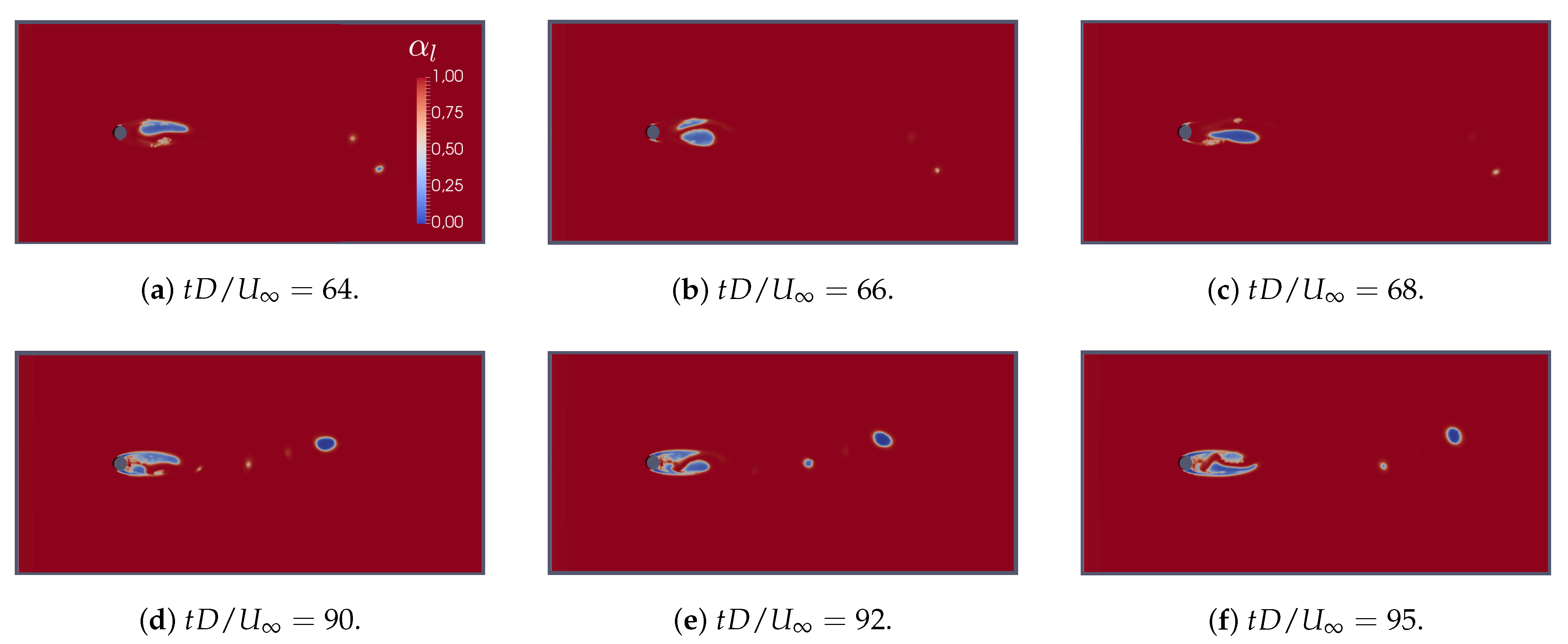
Figure 5 shows snapshots of α l for the simulation carried out with the Kunz model with the standard coefficients, reported in Table 2. During the simulation two alternating scenarios are identified; the first one is the detached cavitation, as depicted in Figure 5a, characterized by two vapor zones that oscillate downstream of the cylinder; the second scenario is the formation and collapse of an attached cavity at the rear of the cylinder, as depicted in Figure 5b–h where it is also noticeable the advection of vapor spots downstream, within the vortex cores. This scenario begins with the detachment of cavities from the cylinder (Figure 5b), they are advected downstream while new vapor forms near the cylinder (Figure 5c,d). The new cavities merge into a single cavity at the rear of the cylinder (Figure 5e,f). The cavity slowly condenses maintaining the position near the cylinder but reducing its extension (Figure 5f,g) until occurrence of complete collapse and the stable detached cavitation is recovered (Figure 5i).
The simulation carried out with the Merkle model (Figure 6) depicts a cavity dynamics comparable to that obtained with the Kunz model, except for the cavity size, which is in general larger than that found with the Kunz model (Figure 6a); the formation of the attached cavity is visible in Figure 6c,d and it appears larger than the one shown in Figure 5e–g.
Figure 7 shows snapshots of the simulation performed with the Saito model, considering the standard coefficients. In this case, the cyclic regime is clear. Indeed, the regular formation of attached cavity is ruled by the vortex shedding, which is nearly unaffected by the small amount of cavitation produced by the model.
Figure 8 shows snapshots of the quantity α l for the simulation performed with the Schnerr-Sauer model. The results show an alternating vapor formation downstream of the cylinder as depicted in the snapshots Figure 8a–c, and the occurrence of extended vaporization at the rear of the body (Figure 8d–i). Figure 8d–f show the development of the attached cavity which occurs starting from the cylinder unlike the simulations with the Kunz (Figure 5) and Merkle (Figure 6) models, where the cavity was formed in the vortex cores. Figure 8g–i show that the vapor cavity at the rear of the cylinder obtained with the Schnerr-Sauer model is more stable and remains attached to the cylinder for a longer period if compared to the other models.
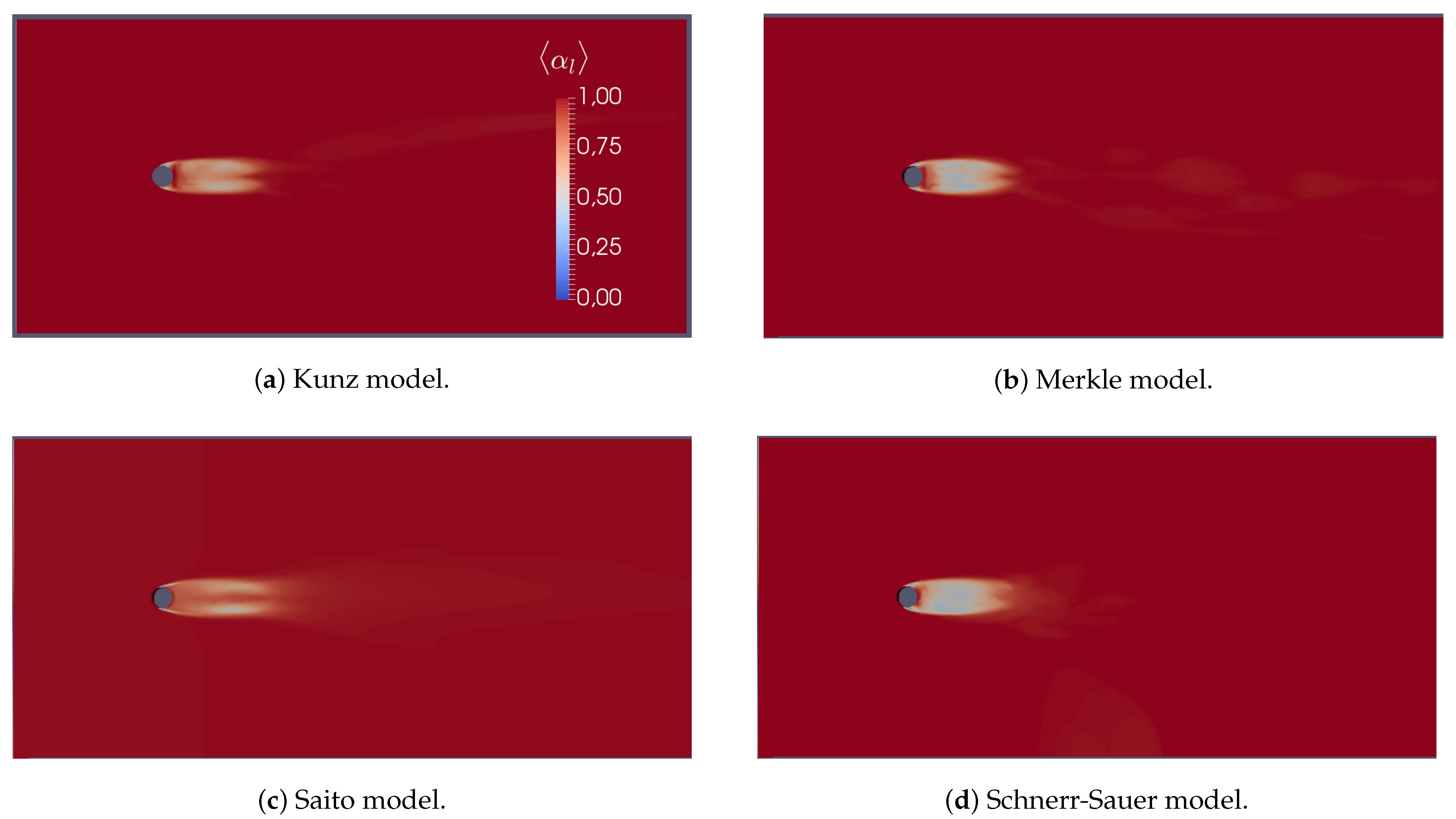
In Figure 9, contours of time-averaged α l are depicted. No particular differences are detected in the shape of the mean cavity. However, the Saito model and, a minor extent the Kunz model, produce a smaller amount of vapor compared to the other models.
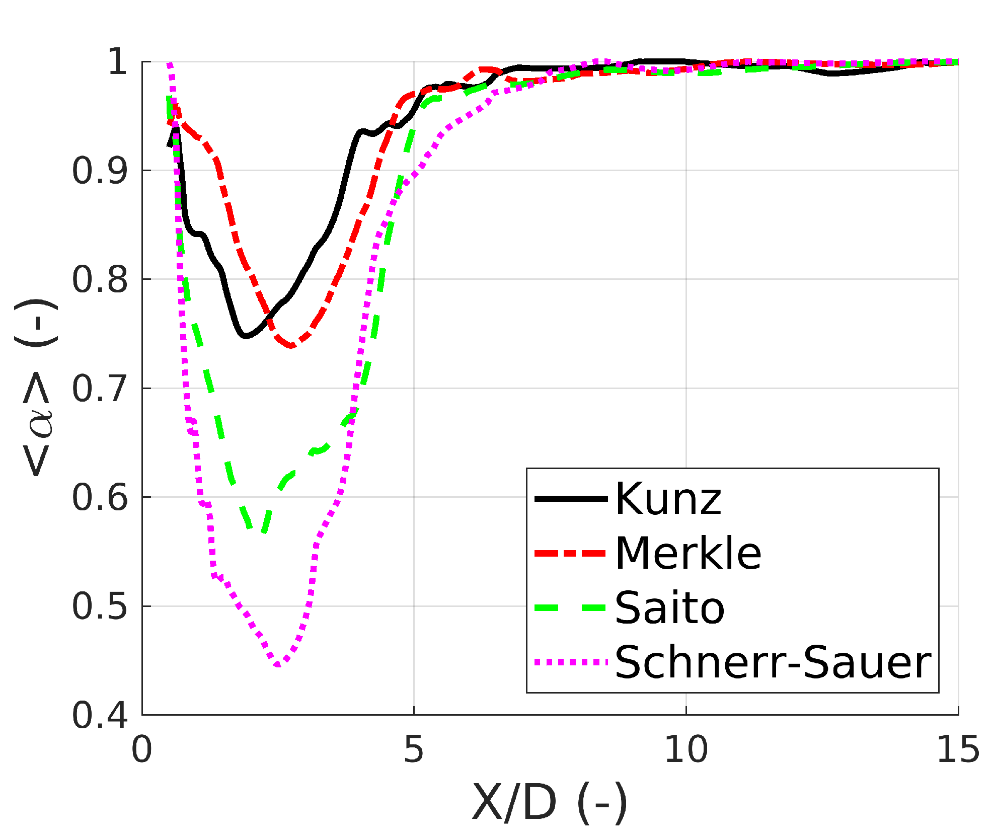
Figure 10 contains the mean vapor fraction plotted along the centerline, downstream the cylinder. The minimum of α l obtained with the Saito model is about α l , m i n = 0.86 . On the other hand, the Saito model produces a longer attached cavity. This means that, unlike the other models, the low condensation rate allows the flow to carry downstream the small amount of vapor produced by the model. This behavior is expected, since the vaporization and condensation rates of the Saito model maintain in time a very low value (see the α l growth and decreasing in time, depicted in Figure 1). The results obtained with Merkle and Schnerr-Sauer models are comparable, due to their similar vaporization and condensation rates. Finally, the Kunz model stands in the middle between the Saito and the others. Indeed, it does not produce a considerable amount of vapor.
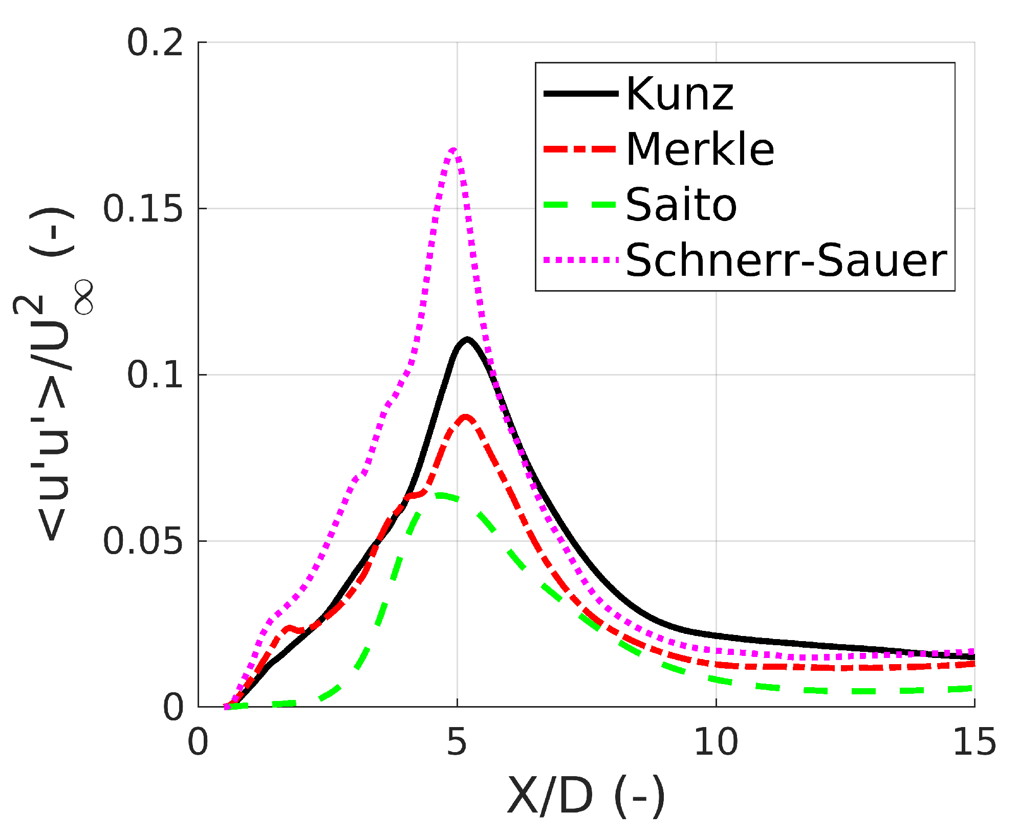
Figure 11 shows the profile of u u / U 2 evaluated along the centerline, downstream the cylinder, being u = u u the fluctuation of the stream-wise velocity component with respect to a time-averaged value (the symbol · denotes an averaging operation). All models show the same behavior, characterized by a single peak located roughly at the same position, except for the Saito model which presents a peak slightly closer to the cylinder. This is consistent with what observed in [26], since a cyclic regime exhibits a vortex shedding similar to the single-phase case, in which the re-attachment point (where u u / U 2 is maximum) is closer to the cylinder with respect to the cavitating case. Furthermore, at the rear of the cylinder u u / U 2 is similar for all models except for the Saito one, which has a lower initial slope. This difference can be explained by the cyclic cavitation regime, in which cavitation has little influence on the vortex shedding, and occurs mainly in the vortex core; in the parametric study of [26] it is noted that as σ decreases from σ = 1 to σ = 0.5 the space derivative of u u / U 2 near the cylinder increases, and the value of the peak changes from a value of about 0.035 to 0.1 with a peak position ranging from 3 D to 7.5 D ; while for values of σ = 0.7 the authors find that the peak is at a position of 4.5 D with a maximum value of about u u / U 2 = 0.07 . The results shown in Figure 11 are consistent with the cavitation regimes depicted in the snapshots of the contour of α l . Indeed the Saito model, which is the only one that exhibits a cyclic regime, is the one with a lower peak, which is also closer to the cylinder, with respect to the other models. Conversely, the Schnerr-Sauer model, which is the one that which produces the most stable attached cavity is the one that has the peak with the highest value.
Figure 12 shows the spectra of the lift coefficient time-history, which gives important information about the frequency of the vortex release. In the present case, broad-band spectra appear and they differ from model to model. This is not surprising, since the dynamics of the cavity behind the cylinder affects the flow field. We note that both the Kunz and Saito models exhibit a well defined main peak at S t = f D / U 0.15 , which is smaller than the value obtained in the single-phase regime; the Merkle and Schnerr-Sauer models give higher values of S t for the peak of C L and broad-band spectra are evident that may be due to pressure fluctuations in the presence of the attached cavity. Given the previous observations (especially about the profile of the time-averaged α l depicted in Figure 10) this is reasonable, in the sense that the low amount of vapor produced by the Kunz and Saito models, slightly affects the oscillatory pattern behind the cylinder.
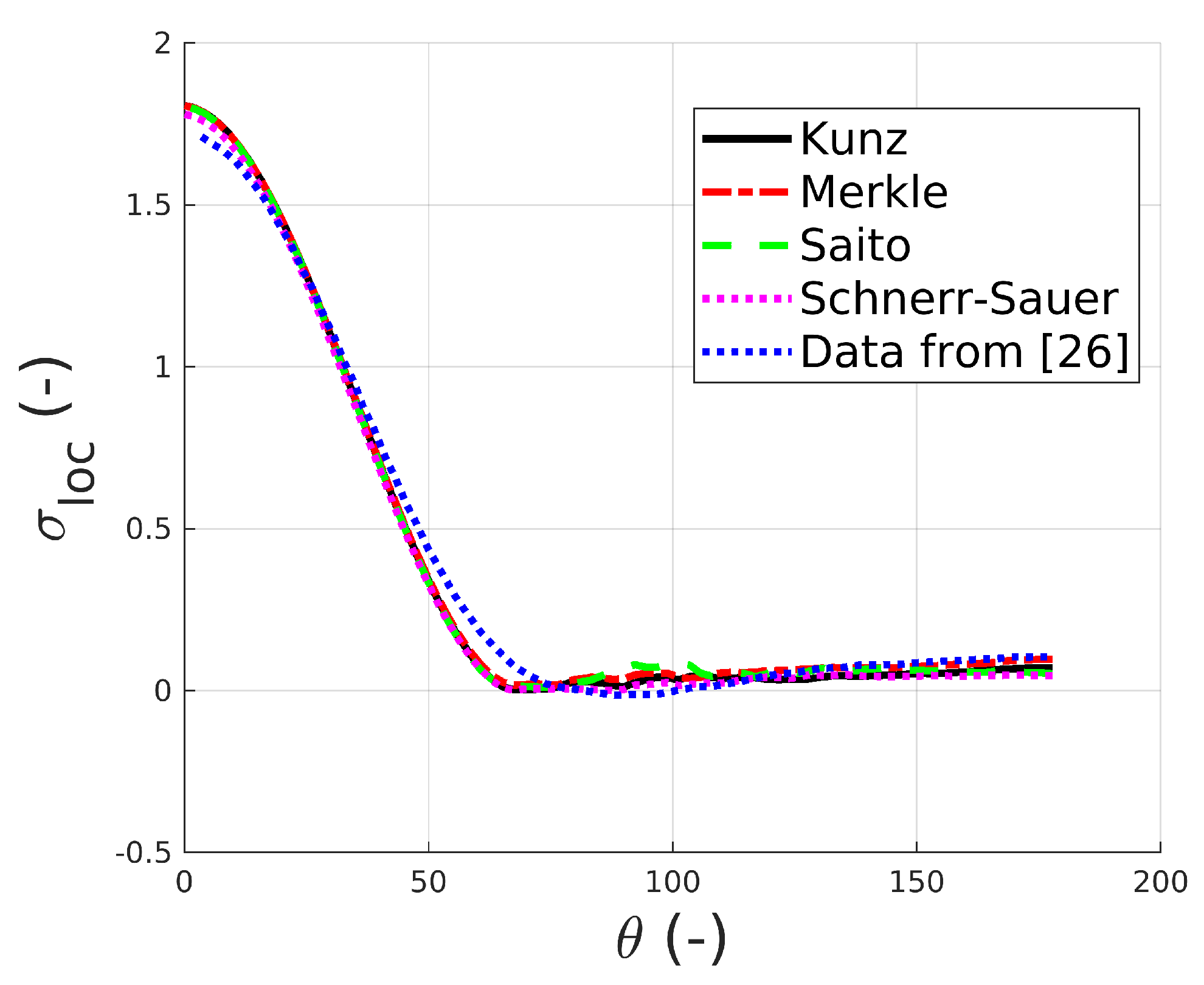
In Figure 13, we report the mean pressure field evaluated over the cylinder surface, related to the four models. We compare our results to those reported in [26]. In Figure 13 we refer to the local σ , which is defined as σ l o c = ( p p v ) / ( 0.5 ρ l U 2 ) as function of θ , defined as angular coordinate of the cylinder surface, where θ = 0 and θ = 180 are the leading edge and the trailing edge, respectively. It appears that in our simulations the incipient cavitation point is shifted a little further upstream than in the reference case [26]. It is also noted that the pressure value upstream of the cylinder is slightly different among the various cases and with respect to the reference value. This may be due to the different pressure boundary conditions adopted, with respect to [26], where the authors imposed the free-stream pressure on all far-field boundaries, while in our case the pressure is imposed at the outlet. In our simulations, we observe significant pressure fluctuations making σ l o c positive, just a little further downstream of the incipient cavitation point. The pressure fluctuations are found to be associated with the collapse of vapor spots and to the variation of the cavity shape.
To quantify the differences observed among the models, we consider the length of the attached cavity, the length of the vortex formation and the vortex shedding frequency. The length of the attached cavity is defined as the position along the centerline where the vapor fraction exceeds the threshold value α l = 0.95 . The length of the vortex formation is defined as the position along the centerline where u u / U 2 reaches the maximum value. The vortex shedding frequency is defined as the frequency associated with the main peak, considering the spectrum of the lift coefficient C L . All quantities are evaluated considering the results of Figure 10, Figure 11 and Figure 12. In [26], the authors found that for σ = 0.7 , the minimum value of the mean liquid fraction is about 0.8 with an attached cavity length of about 5 D . In our study, we find that the length of attached cavity varies within the range 4.1 D , 6.3 D being the minimum of mean liquid fraction α l , m a x in the range 0.45 , 0.85 . The variance exhibits peaks in the range ( u u / U 2 ) m a x [ 0.06 , 0.17 ] , located at distances varying from 4.7 D to 5.2 D .
In Table 8, we report the length of the attached cavity, the vortex formation length and the vortex shedding frequency, related to the four models.
To summarize, results show that although the time-averaged liquid fraction does not exhibit noticeable differences among models, the snapshots and the other quantities above reported reveal a substantially different behavior of the cavitation. The Saito model is characterized by low values of vapor fraction which do not affect the flow field, rather they are affected by it, being transported downstream. This is identified as a cyclic regime. The Schnerr-Sauer model seems to be the one that has the most stable attached cavitation alternating with periods of detached cavitation, exhibiting a well defined transitional regime. Merkle and Kunz models behave similarly, having a predominant detached cavitation, with some phases of attached cavitation but very unstable and of short duration.
It should be noted that especially the spatial distribution of the mean liquid fraction and the variance of the stream-wise velocity component obtained with the Saito model are closer to the results obtained numerically in [26] who used the same method in conjunction with a compressible-flow solver.

5.2. Analytical-Based Coefficients

We now discuss the results of the simulations performed considering the coefficients C c and C v calculated as described in Section 3. We emphasize that, since the Schnerr-Sauer model was taken as a reference to compute time scales T c , r e f and T v , r e f , results and observations concerning the Schnerr-Sauer simulation are the same reported in the previous Section 5.1.
Snapshots of the liquid vapor fraction α l obtained with the Kunz model with calculated coefficients are depicted in Figure 14. We observe a transitional regime with a predominant detached cavitation (Figure 14a–c). It is worth noting that, with the calculated coefficients, after the detachment of the vapor zones an attached cavity originates directly from the cylinder (Figure 14d) and extends downstream (Figure 14e,f) for a short period but fails in developing a stable attached cavity at the rear of the cylinder.
In Figure 15 we show snapshots of the liquid fraction obtained with the Merkle model, considering calculated coefficients (Table 3). Both detached (Figure 15a–c) and attached cavitation (Figure 15d–f) are visible. In this case, the vapor spots appear narrower than those observed in Figure 6 obtained with the standard coefficients, producing a different profile of the mean α l along the centerline, as it will be shown in the following. Regions of attached cavities are still visible, albeit of smaller extension and for a shorter period, but generated from the cylinder itself, and extending downstream (Figure 15d–f); the shape of cavitation is very similar to that obtained with the Kunz model with calculated coefficients.
Figure 16 shows snapshots of α l from the simulation performed with Saito’s model with the calculated coefficients, reported in Table 3. The new coefficient set up makes the cavity dynamics of Saito model similar to that observed with the other models, in particular with that of Schnerr-Sauer one. Indeed, the cyclic regime disappears, and both detached and attached cavitation occur (see, respectively, Figure 16a–c and Figure 16d–f).
In Figure 17, the time-averaged liquid fraction α l is depicted. We note that the behavior of the cavitation is similar for all models; the main difference with respect to the standard-coefficients case is observed for the Saito model which, as expected, in this case exhibits a more intense vapor phase.
Figure 18 shows the mean liquid fraction evaluated along the centerline, downstream the cylinder. The models of Merkle and Kunz behave similarly to each other. Conversely, the models of Saito and Schnerr-Sauer produce more vapor fraction than the others. The difference is due to the cavitation regime reproduced by the models; in the case of Kunz and Merkle it is transitional with a strong prevalence of the detached component mainly distributed on the sides with respect to the centerline; the Saito and Schnerr-Sauer models produce a transitional regime but with a more stable cavity which occupies the central area at the rear of the cylinder and a higher percentage of mean vapor.
Figure 19 shows the variance of the stream-wise component of the velocity u u / U 2 . The figure shows that with the new coefficients, the Saito model tends to give results more similar to those of the other models. As observed in [26], when cavitation moves from a cyclic regime to a transitional one, the peak of u u / U 2 moves downstream and their value increases, coherently with the cavitation regime observed. The variance has practically the same behavior for all models in the area immediately downstream the cylinder and is characterized by a linear increase. For this quantity we note that the Kunz model produces a peak a bit more downstream then the other models, although it behaves similarly to the Schnerr-Sauer model in the far-field.
Figure 20 shows the spectra of the lift coefficients. All models exhibit a broad-band behavior, making the computation of the Strouhal number not straightforward. The Schnerr-Sauer model has the main peak not coincident with those of the others, while all the other models has practically the same value for the vortex shedding frequency. The values observed are consistent with literature, since the Strouhal number for the single-phase case is S t = 0.2 , and it decreases as the cavitation number decreases.
Figure 21 shows the mean pressure over the cylinder; the analytical evaluation of the coefficients leads to more similar values of pressure both in the upstream stagnation point and in the downstream region, where all models give pressure values in between the Schnerr-Sauer model and the literature value [26]. Furthermore, in this case we observe the presence of spots of positive value of the mean σ l o c , for θ [ 80 , 120 ] ; for this quantity as well, we note that the models with the coefficients calculated analytically have a more consistent behavior.
For all simulations, the length of the attached cavity, the length of vortex formation and the vortex shedding frequency were evaluated from the data shown, respectively, in Figure 18, Figure 19 and Figure 20. The quantities are collected in Table 9.
As a final analysis, in order to quantify the differences among the results given by the models before and after computation of the coefficients, we calculate the variance between the results for the three quantities, and the values obtained are gathered in Table 10.
The variance of the length of vortex formation undergoes a slight deterioration after the direct calculation of the coefficients. On the other hand, for the length of the attached cavity, and the mean vapor fraction downstream of the cylinder, it can be observed that after computation of the coefficients, the models behave much more similarly, as it can be seen from the comparison between Figure 9 and Figure 17. It is noted that the variance between the results decreases by almost 70 % once the coefficients are calculated directly using the procedure suggested in the present paper. Moreover, we note that with the new coefficients all models exhibit a broad-band behavior for the spectra of the lift coefficient and the vortex shedding frequency evaluated appears much more similar among the models, which leads to a variance that is one order of magnitude lower than that obtained for the standard coefficients.
The results shown above indicate that the analytical evaluation of the coefficients of the model improve the quality of the results. This is mainly evident for the Saito model. The Kunz and Merkle models behave very similarly and exhibit differences with the Schnerr-Sauer model. This may be due to the derivative of α (see right panel of Figure 2) which changes dramatically from the Kunz and Merkle models to the Saito and Schnerr-Sauer models. Finally, we performed a grid-sensitivity test, considering a grid coarser than that discussed in the present Section. The analysis (herein not described in detail) shows that the analytical evaluation of the coefficients provides some improvement in the results even in the presence of a coarse mesh, although better results are obtained with a good quality mesh.

6. Concluding Remarks /Summary

In this study, we propose a novel analytical approach to calculate the coefficients of cavitation models, based on the reference time needed for vaporization/condensation processes, from a volume fraction α 0 to a value α 1 , in a archetypal situation characterized by a constant pressure field and neglecting advective transport. This approach was then tested for four different models (Kunz, Merkle, Saito, and Schnerr-Sauer) considering the two-dimensional laminar flow around a circular cylinder. The simulations were performed both with standard literature coefficients and with the new values calculated using this new approach. The results were analyzed and compared on the basis of the consistency for the various models and with respect to a literature case [26] as regards various characteristics and physical quantities of the simulations; in particular, for each model, we first evaluated the cavitation regime reproduced and successively we have calculated the mean pressure over the cylinder, the length of the attached cavity, the length of vortex formation and the vortex shedding frequency. It was noticed that, as a result of the analytical evaluation of the coefficients, for some models there is a considerable improvement of the results regarding the cavitation regime and the reference quantities above reported, in particular for the Saito model; specifically the Saito model used with the standard coefficients was found to predict a cyclic regime instead of the transitional one reproduced by the other models; the same model, with the analytically calculated coefficients predicts a transitional regime with a more stable attached cavity, likewise the Schnerr-Sauer model, which in our study has been taken as a reference for the evaluation of the reference times for condensation/vaporization. Regarding the Kunz and Merkle models, it was found that after the analytical evaluation of the coefficients the two models behave similarly to each other, even if they behave differently from the Schnerr-Sauer model, in that they fail to develop the stable cavity attached on the rear of the cylinder. Specifically an attached cavity tries to form in contact with the cylinder but it rapidly disappears. On the other hand, the use of standard values of the coefficients leads to development of a cavitation region at the rear of the cylinder, from the vapor present in the vortices and collapsing shortly after. Overall, this preliminary study shows that the use of analytically based coefficients significantly improves the performance of some models, while for others the improvement was not so evident; this may be due to different reasons: among them, the range of values for the volume fraction used to calculate the coefficients, the fact that the condensation and evaporation time scales are assumed to be the same, and, finally, the fact that the reference model herein used (Schnerr-Sauer model) is already a simplified model derived from the more complete and physical-based Rayleigh-Plesset equation. Currently we are carrying out additional analysis on this matter, which will be the subject of a future paper.

Author Contributions

Conceptualization, A.S., M.C. and V.A.; methodology, A.S.; validation, A.S.; formal analysis, A.S.; investigation, A.S. and M.C.; data curation, A.S.; writing—original draft preparation, A.S.; writing—review and editing, A.S., M.C. and V.A.; visualization, A.S.; supervision, M.C. and V.A. All authors have read and agreed to the published version of the manuscript.

Funding

This research was supported by Fondo Sociale Europeo della Regione autonoma Friuli Venezia Giulia, Universitá degli studi di Trieste and Finanziamento di Ateneo per progetti di ricerca scientifica–D13-FRA-2021.

Institutional Review Board Statement

Not applicable.

Informed Consent Statement

Not applicable.

Conflicts of Interest

The authors declare no conflict of interest.

References

  1. Brennen, C. Cavitation and Bubble Dynamics; Oxford University Press: Oxford, UK, 1995. [Google Scholar]
  2. D’Agostino, L.; Salvetti, M.V. Fluid Dynamics of Cavitation and Cavitating Turbopumps; CISM International Centre for Mechanical Sciences; Springer: Vienna, Austria, 2008. [Google Scholar]
  3. Plesset, M.; Prosperetti, A. Bubble Dynamic and Cavitation. Ann. Rev. Fluid Mech. 1977, 9, 145–185. [Google Scholar] [CrossRef]
  4. Tzanakis, I.; Eskin, D.G.; Georgoulas, A.; Fytanidis, D.K. Incubation pit analysis and calculation of the hydrodynamic impact pressure from the implosion of an acoustic cavitation bubble. Ultrason. Sonochem. 2014, 21, 866–878. [Google Scholar] [CrossRef] [PubMed]
  5. Petkovšek, M.; Dular, M. Simultaneous observation of cavitation structures and cavitation erosion. Wear 2013, 300, 55–64. [Google Scholar] [CrossRef]
  6. Salio, M.P. Numerical assessment of underwater noise radiated by a cruise ship. Ships Offshore Struct. 2015, 10, 308–327. [Google Scholar] [CrossRef]
  7. Tryggvason, G.; Bunner, B.; Esmaeeli, A.; Juric, D.; Al-Rawahi, N.; Tauber, W.; Hanc, J.; Nas, S.; Jan, Y.-J. A Front-Tracking Method for the Computationsof Multiphase Flow. J. Comput. Phys. 2001, 169, 708–759. [Google Scholar] [CrossRef] [Green Version]
  8. Yakubov, S.; Cankurt, B.; Abdel-Maksoud, M.; Rung, T. Hybrid MPI/OpenMP parallelization of an Euler–Lagrange approach to cavitation modelling. Comput. Fluids 2013, 80, 365–371. [Google Scholar] [CrossRef]
  9. Ghahramani, E.; Ström, H.; Bensow, R. Numerical simulation and analysis of multi-scale cavitating flows. J. Fluid Mech. 2021, 922, A22. [Google Scholar] [CrossRef]
  10. Delannoy, Y.; Kueny, J.L. Two phase flow approach in unsteady cavitation modeling. ASME Cavitation Multiph. Flow Forum 1990, 109, 153–159. [Google Scholar]
  11. Reboud, J.L.; Stutz, B.; Coutier-Delgosha, O. Two phase flow structure of cavitation: Experiment and modeling of unsteady effects. In Proceedings of the 3rd International Symposium on Cavitation, Grenoble, France, 7–10 April 1998. [Google Scholar]
  12. Song, C.; He, G. Numerical simulation of cavitating flow by single-phase flow approach. In Proceedings of the 3rd International Symposium on Cavitation, Grenoble, France, 7–10 April 1998. [Google Scholar]
  13. Coutier-Delgosha, O.; Fortes-Patella, R.; Reboud, J.L.; Hakimi, N.; Hirsch, C. Stability of preconditioned Navier–Stokes equations associated with a cavitation model. Comput. Fluids 2005, 34, 319–349. [Google Scholar] [CrossRef]
  14. Qin, Q.; Song, C.C.S.; Arndt, R.E.A. A virtual single-phase natural cavitation model and its application to Cav2003 hydrofoil. In Proceedings of the 5th International Symposium on Cavitation, Osaka, Japan, 1–4 November 2003. [Google Scholar]
  15. Merkle, C.L.; Feng, J.; Buelow, P.E.O. Computational modelling of the dynamics of sheet cavitation. In Proceedings of the 3rd International Symposium on Cavitation, Grenoble, France, 7–10 April 1998. [Google Scholar]
  16. Kunz, R.F.; Boger, D.A.; Stinebring, D.R.; Chyczewski, T.S.; Lindau, J.W.; Gibeling, H.J.; Venkateswaran, S.; Govindan, T.R. A preconditioned Navier–Stokes method for two-phase flows with application to cavitation prediction. Comput. Fluids 2000, 29, 849–875. [Google Scholar] [CrossRef]
  17. Senocak, I.; Shyy, W. Evaluation of cavitation models for Navier–Stokes Computations. In Proceedings of the FEDSM2002,02 ASME Fluids Engineering Division Summer Meeting, Montreal, QC, Canada, 14–18 July 2002. [Google Scholar]
  18. Singhal, A.K.; Vaidya, N.; Leonard, A.D. Multi-dimensional simulation of cavitating flows using a PDF model for phase change. In Proceedings of the ASME Fluids Engineering Division Summer Meeting, Vancouver, BC, Canada, 22–26 June 1997. [Google Scholar]
  19. Zwart, P.J.; Gerber, A.G.; Belamri, T. A two-phase flow model for predicting cavitation dynamics. In Proceedings of the International Conference on Multiphase Flow, Yokohama, Japan, 30 May–4 June 2004. [Google Scholar]
  20. Schnerr, G.H.; Sauer, J. Physical and Numerical Modeling of Unsteady Cavitation Dynamics. In Proceedings of the 4th International Conference on Multiphase Flow, New Orleans, LA, USA, 27 May–1 June 2001. [Google Scholar]
  21. Saito, Y.; Takami, R.; Nakamori, I.; Ikohagi, T. Numerical analysis of unsteady behavior of cloud cavitation around a NACA0015 foil. Comput. Mech. 2007, 40, 85–96. [Google Scholar] [CrossRef]
  22. Roohi, E.; Zahiri, A.P.; Passandideh-Fard, M. Numerical simulation of cavitation around a two-dimensional hydrofoil using VOF method and LES turbulence model. Appl. Math. Model. 2013, 37, 6469–6488. [Google Scholar] [CrossRef]
  23. Morgut, M.; Nobile, E. Numerical Predictions of Cavitating Flow around Model Scale Propellers by CFD and Advanced Model Calibration. Int. J. Rotating Mach. 2012, 2012, 618180. [Google Scholar] [CrossRef]
  24. Zhou, H.; Xiang, M.; Okolo, P.; Wu, Z.; Bennett, G.; Weihua, Z. An efficient calibration approach for cavitation model constants based on OpenFOAM platform. J. Mar. Sci. Technol. 2019, 24, 1043–1056. [Google Scholar] [CrossRef]
  25. Gaggero, S.; Villa, D. Steady cavitating propeller performance by using OpenFOAM, StarCCM+ and a boundary element method. Proc. Inst. Mech. Eng. Part M J. Eng. Marit. Environ. 2017, 231, 411–440. [Google Scholar] [CrossRef]
  26. Gnanaskandan, A.; Mahesh, K. A numerical method to simulate turbulent cavitating flows. Int. J. Multiphase Flow 2015, 70, 22–34. [Google Scholar] [CrossRef]
  27. Lu, N. Available online: http://www.tfd.chalmers.se/~hani/kurser/OS_CFD_2008/NaixianLu/REPORT_interPhaseChangeFoam.pdf (accessed on 2 June 2021).
  28. Kundu, P.K. Fluid Mechanics; Elsevier: New York, NY, USA, 1990. [Google Scholar]
  29. Fry, S. Investigating cavity/wake dynamics for a circular cylinder by measuring noise spectra. J. Fluid Mech. 1984, 142, 187–200. [Google Scholar] [CrossRef]
  30. Matsudaira, Y.; Gomi, Y.; Oba, R. Characteristics of bubble-collapse pressures in a Karman-vortex cavity. JSME Int. J. 1992, 35, 179–185. [Google Scholar] [CrossRef] [Green Version]
Figure 1. Condensation (left panel) and vaporization (right panel) processes, evaluated with standard coefficients.
Energies 14 06425 g001
Figure 2. Condensation and vaporization processes with analytical-based coefficients.
Energies 14 06425 g002
Figure 3. Schematic of the computational domain.
Energies 14 06425 g003
Figure 4. Near body mesh used for the simulations.
Energies 14 06425 g004
Figure 5. Contour plot of instantaneous liquid fraction obtained with Kunz model and considering standard coefficients.
Energies 14 06425 g005
Figure 6. Contour plot of instantaneous liquid fraction, results obtained with Merkle model and considering standard coefficients.
Energies 14 06425 g006
Figure 7. Contour plot of instantaneous liquid fraction, results obtained with Saito model and considering standard coefficients.
Energies 14 06425 g007
Figure 8. Contour plot of instantaneous liquid fraction, results obtained with SchnerrSauer model and considering standard coefficients.
Energies 14 06425 g008
Figure 9. Contour plot of time-averaged liquid fraction, results obtained considering standard coefficients.
Energies 14 06425 g009
Figure 10. Mean liquid fraction downstream the cylinder along the centerline, results obtained considering standard coefficients.
Energies 14 06425 g010
Figure 11. Variance of stream-wise velocity component downstream the cylinder along the centerline, results obtained considering standard coefficients.
Energies 14 06425 g011
Figure 12. Lift coefficient, results obtained considering standard coefficients (Table 2).
Energies 14 06425 g012
Figure 13. Time averaged local σ on the cylinder surface, results obtained considering standard coefficients (Table 2).
Energies 14 06425 g013
Figure 14. Contour plot of instantaneous liquid fraction, results obtained with Kunz model and considering analytical-based coefficients (Table 3).
Energies 14 06425 g014
Figure 15. Contour plot of instantaneous liquid fraction, results obtained with Merkle model and considering analytical-based coefficients (Table 3).
Energies 14 06425 g015
Figure 16. Contour plot of instantaneous liquid fraction, results obtained with Saito model and considering analytical-based coefficients (Table 3).
Energies 14 06425 g016
Figure 17. Contour of time-averaged liquid fraction, results obtained considering analytical-based coefficients.
Energies 14 06425 g017
Figure 18. Mean liquid fraction downstream the cylinder along the centerline, results obtained considering analytical-based coefficients.
Energies 14 06425 g018
Figure 19. Variance of stream-wise velocity component downstream the cylinder along the centerline, with analytical-based coefficients.
Energies 14 06425 g019
Figure 20. Lift coefficient spectrum with analytical-based coefficients.
Energies 14 06425 g020
Figure 21. Time averaged local σ on the cylinder surface considering analytical-based coefficients.
Energies 14 06425 g021
Table 1. Source terms for the non-conservative form of the transport Equation (Equation (3)), according to the cavitation models considered.
Model m ˙ m ˙ +
Kunz C c ρ ρ l α l 2 ( 1 α l ) t max ( p p v , 0 ) | p p v | C v ρ ρ l 2 α l max ( p v p , 0 ) 1 2 U 2 t
Merkle C c ρ ρ l ρ v ( 1 α l ) max ( p p v , 0 ) 1 2 U 2 t C v ρ ρ v 2 α l max ( p v p , 0 ) 1 2 U 2 t
Saito C c ρ ρ l ρ v α l 2 ( 1 α l ) 2 max ( p p v ) 2 π R T g C v ρ ρ v 2 α l 2 ( 1 α l ) 2 max ( p v p ) 2 π R T g
Schnerr-Sauer C c 3 α l ( 1 α l ) R b 2 3 max ( p p v , 0 ) ρ l C v 3 α l ( 1 α l ) R b 2 3 max ( p v p , 0 ) ρ l
Table 2. Standard coefficients.
Model C c C v
Kunz10001000
Merkle80 1 × 10 3
Saito 0.1 0.1
Schnerr-Sauer11
Table 3. Analytical-based coefficients.
Model C c C v
Kunz 4.11 × 10 4 2.91 × 10 6
Merkle 3.33 × 10 1 1.55 × 10 3
Saito 3.75 × 10 5 8.66
Schnerr-Sauer11
Table 4. Details on the computational domain considered.
CharacteristicSymbolValueDimension
DiameterD1(m)
Domain length total 32(m)
Domain upstream length 7(m)
Domain width 15(m)
Table 5. Boundary conditions for the simulation of the two-dimensional laminar flow around the cylinder.
Boundary α l up
Inletuniform 0.99 uniform ( 1 , 0 ) m/szero gradient
Outletzero gradientzero gradientuniform 2650 Pa
Cylinderzero gradientuniform 0 m/szero gradient
Lateral boundarieszero gradientzero gradientzero gradient
Table 6. Fluid data considered in simulations.
CharacteristicSymbolValueDimension
Reynolds number R e 200(-)
Cavitation index σ 0.7 (-)
Liquid density ρ l 1000(kg/m 3 )
Liquid kinematic viscosity ν l 0.005 (m 2 /s)
Vapor density ρ v 0.023 (kg/m 3 )
Vapor kinematic viscosity ν v 2.374 (m 2 /s)
Vapor pressure p v 2300(Pa)
Input velocity U 1(m/s)
Output pressure p 0 2650(Pa)
Table 7. Set up of parameters contained in the cavitation models.
CharacteristicSymbolValueDimension
Velocity U 1(m/s)
Reference time t 1(s)
Gas costantR 461.6 (J/(Kg K))
Temperature T g 300(K)
Free nuclei densityn 1.6 × 10 13 (1/m 3 )
Free nuclei diameter d n u c 2 × 10 6 (m)
Table 8. Length of attached cavity, vortex formation length and non-dimensional vortex shadding frequency. Results obtained considering standard coefficients.
ModelMean Length of Attached CavityVortex Formation LengthVortex Shadding Frequency
Kunz 4.17 D 5.20 D 0.149
Merkle 4.63 D 5.15 D 0.240
Saito 6.24 D 4.68 D 0.134
Schnerr-Sauer 5.98 D 4.93 D 0.165
Table 9. Results of length of attached cavity, vortex formation length and non-dimensional vortex shedding frequency with analytical-based coefficients.
ModelMean Length of Attached CavityVortex Formation LengthVortex Shadding Frequency
Kunz 4.96 D 5.60 D 0.194
Merkle 4.66 D 5.07 D 0.195
Saito 5.10 D 5.01 D 0.195
Schnerr-Sauer 5.98 D 4.93 D 0.165
Table 10. Variances for the results of length of attached cavity, vortex formation length and vortex shedding frequency for standard and analytical-based coefficients.
Length of Attached CavityVortex Formation LengthVortex Shadding Frequency
Standard coefficients 0.766 0.042 1.64 × 10 3
Analytical-based coefficients 0.241 0.069 1.66 × 10 4
Publisher’s Note: MDPI stays neutral with regard to jurisdictional claims in published maps and institutional affiliations.

