Thermodynamic Analysis of Negative CO₂ Emission Power Plant Using Aspen Plus, Aspen Hysys, and Ebsilon Software

Abstract

The article presents results of thermodynamic analysis using a zero-dimensional mathematical models of a negative CO₂ emission power plant. The developed cycle of a negative CO₂ emission power plant allows the production of electricity using gasified sewage sludge as a main fuel. The negative emission can be achieved by the use this type of fuel which is already a “zero-emissive” energy source. Together with carbon capture installation, there is a possibility to decrease CO₂ emission below the “zero” level. Developed models of a novel gas cycle which use selected codes allow the prediction of basic parameters of thermodynamic cycles such as output power, efficiency, combustion composition, exhaust temperature, etc. The paper presents results of thermodynamic analysis of two novel cycles, called PDF0 and PFD1, by using different thermodynamic codes. A comparison of results obtained by three different codes offered the chance to verify results because the experimental data are currently not available. The comparison of predictions between three different software in the literature is something new, according to studies made by authors. For gross efficiency (54.74%, 55.18%, and 52.00%), there is a similar relationship for turbine power output (155.9 kW, 157.19 kW, and 148.16 kW). Additionally, the chemical energy rate of the fuel is taken into account, which ultimately results in higher efficiencies for flue gases with increased steam production. A similar trend is assessed for increased CO₂ in the flue gas. The developed precise models are particularly important for a carbon capture and storage (CCS) energy system, where relatively new devices mutually cooperate and their thermodynamic parameters affect those devices. Proposed software employs extended a gas–steam turbine cycle to determine the effect of cycle into environment. First of all, it should be stated that there is a slight influence of the software used on the results obtained, but the basic tendencies are the same, which makes it possible to analyze various types of thermodynamic cycles. Secondly, the possibility of a negative CO₂ emission power plant and the positive environmental impact of the proposed solution has been demonstrated, which is also a novelty in the area of thermodynamic cycles.

1. Introduction

Decarbonization of the economy, specifically in energy generation sector, has been adopted as a world-wide policy with signing of the Paris Agreement by nearly 200 signatories, including most significant emitters [1]. Thus, an ambitious greenhouse gases reduction goals has been set, in order to prevent the average global temperature increasing more than 1.5 °C above the pre-industrial levels [1]. An extensive effort is needed to achieve such goal [2]. Fossil fuels contributed approximately 9.5 Gt of carbon emitted to the atmosphere on average per year, as highlighted by the global carbon budget for years 2009–2018 [3].

The United Nations Framework Convention on Climate Change (UNFCCC) has recognized carbon capture and storage (CCS) technologies as important means of achieving ambitious climate goals [4]. Parameters, such as efficiency, cost, and water, have been considered as extremely important factors, determining the success of CCS technologies [5]. The work completed on CCS so far has been focused on post-combustion CCS [6], its integration with power plants [7,8], and combustion with different oxygen concentrations, since dilution of CO₂ in flue gases influences capturing efficiency [9,10]. Furthermore, various emerging CCS technologies, such as membrane-based carbon capture and storage [11], pre-combustion CO₂ capture [12], or carbon sequestration in hydrates [13,14,15], are also subjects of intensive investigations.

1.1. Concept of Negative Emissions Power Plants Using Biomass

The concept of achieving negative emissions has recently caught some attention [16]. Using biomass, combined with CCS, to achieve negative CO₂ emissions, it is often described as bioenergy with carbon capture and storage (BECSS) [17]. Investigative efforts have been mainly focused on chemical looping combustion (CLC) of biomass [18], as well as co-combustion with coal [19]. Lyngfelt et al. [20] investigated possibilities of leakages of stored CO₂ and concluded that, due to expected time scales of such events, the contribution of such leakages to the atmospheric stock would be relatively small, reaching approximately 3 ppm of CO₂ [20]. The use of different types of biomass has been investigated, including the work of Niu et al. [21] on CLC of sewage sludge. Saari et al. [22] investigated BECSS, using CLC with oxygen uncoupling dedicated to large scale co-generation plant. The results have shown an extremely small efficiency penalty of 0.7%, along with CO₂ capturing efficiency being as high as 97% [22].

Nonetheless, other ways to practically apply BECSS are also being investigated. Lisbona et al. [17] evaluated synergy between biogas plant and a biomass power plant, with special attention to the CCS module. Proposed installation, utilizing 1.5 MW of biomass and 1.4 MW of biogas (power as chemical energy at the inlet), was able to generate 750 kW_el of electricity and generate 600 kW_th of heat, for its own needs [17]. Additionally, the installation was able to capture 1620 tons of CO₂ per year [17]. Buscheck and Upadhye [23] investigated hybrid approach, incorporating oxy-combustion and heat accumulation. Such a concept is important, not only from the point of view of negative CO₂ emissions, but also from the point of view of limiting the curtailment of energy generation using intermittent renewable energy sources [23], as flexibility is critical for power systems with high shares of intermittent renewable energy sources (solar, wind) [24,25,26,27,28]. Capron et al. [29] focused on the use of Allam Cycle for achieving carbon negative emissions. A comprehensive overview, as presented in that paper, suggested that CCS could be combined with growing seafood, its subsequent processing, and production of biofuels, resulting in simultaneous increase in productivity and decrease in the exploited surface of the oceans, thus increasing the overall areas dedicated to conservation of biodiversity [29].

However, practical application of BECSS solution could be costly. Cheng et al. [30] determined levelized costs of different BECSS solutions for the US state of Virginia reaching USD/ton_CO2 82 (approx. EUR 70) for combustion of crop residues and USD/ton_CO2 137 (approx. EUR 115) for combustion of woody residues. This is still much less than the current market value that could be assigned for a ton of avoided CO₂ emissions [31]. However, a study performed by Restrepo-Valencia and Walter [32] indicates that EUR/ton_CO2 59 can be achieved for optimized BECSS using bagasse and the cost could be further decreased to EUR/ton_CO2 48 for larger plants. This suggests that significant amount of work is needed to optimize BECSS in terms of CAPEX and OPEX. Such goal can be achieved by optimization of such systems, by comprehensive thermodynamic analysis.

1.2. Software for Zero-Dimensional Modelling

The zero-dimensional approach is mainly used for systems optimization. A limited amount of the obtained data makes it possible to conduct many optimizing calculations of the turbine parameters or entire complex system composed of many devices, such as compressors, expanders, heat exchangers, combustion chambers, reactors, fuel cells, pumps, or ejectors.

Literature on different software is very extensive; however, the most widely used ones are presented below, as follows:

• Aspen Plus is intended for a combined system, steam cycle, ORC cycle; operation under 50–110% nominal load [33];
• Aspen Hysys is intended for a combined system; operation under 50–110% nominal load and dynamic conditions [34];
• Ebsilon is designed for advanced steam block systems and combined systems, operation under variable conditions 40–120% of nominal load [35,36];
• Gate Cycle is designed for advanced combination systems, variable load operation 40–120% of nominal load [37];
• COM-GAS is intended for design level of combined systems with full analysis of a heat recovery steam generator, pulverized fuel, and fluidized bed boilers [38,39];
• DIAGAR is intended for design and diagnostic level of steam systems with full steam turbine analysis [40];
• IPSEpro is a process simulation tool, which is equation-oriented and has been used for power plant simulations, including modeling of chemical looping CCS systems [22];

The most important issue about software for thermodynamic cycles is that they have a high degree of certainty and confidence in the calculation results, which are only achieved by highly validated codes. This means that such codes, in addition to basic calculation algorithms, have extensive expert procedures for checking the results before they are passed on to the user. We selected three codes for detailed analysis of the considered case, namely Aspen Plus, Aspen Hysys, and Ebsilon. The following subsections provide a literature review on these codes.

1.3. Scope and Aim

The main objective of this paper is to analyze an innovative technology together with the proof of concept, confirming the possibility of the use of sewage sludge to produce electricity while having a positive impact on the environment. The synergy between the CCS plant and the proposed utilization of sewage sludge (which is considered a renewable energy source) enables the installation to achieve overall negative emissions of CO₂ (nCO2PP). Proposed processes of utilization (PFD0—Section 2 and Section 3; PFD1—Section 4 and Section 5), called nCO2PP (negative CO₂ Power Plant), ensures reaching of scientific objectives related to three essential theoretical elements, namely: (1) a system that processes sewage sludge into syngas; (2) a system that burns the resulting fuel in pure oxygen in a dedicated wet combustion chamber; and (3) a system of a unique turbine cooperating with a spray ejector condenser with carbon dioxide capture.

The second aim of the article is to compare the results obtained in three computing codes, namely Aspen Plus, Aspen HYSYS, and Ebsilon, based on the assumption presented in next section, and subsequently pointing out the differences and identifying the reasons for them. Section 2 examines the original simple system consisting of an arrangement of equipment such as compressors, expanders, heat exchanger, combustion chamber, pump, and generator to generate electrical energy. A schematic of the cycle can be found in Figure 1, while Figure 2 presents the model in Aspen Hysys, Figure 3 in Aspen plus, and Figure 4 in Ebsilon. Section 3 presents the following subsections as follows: (1) thermodynamic parameters and mass flow rates in nodal points; (2) the output and efficiencies of power; and (3) the effect of NO_x production on combustion chamber temperature. In Section 4, this system is extended to include a spray ejector condenser, where diagrams of power output, efficiency, and chemical energy flow delivered to the combustion chamber are prepared for clarity of results. In Section 5, it is shown that this gas-fired power plant, after the use of gasification fuel (the composition of mixture 1 is given as an example), is CO₂-negative. The last section summarizes the work carried out and draws conclusions.

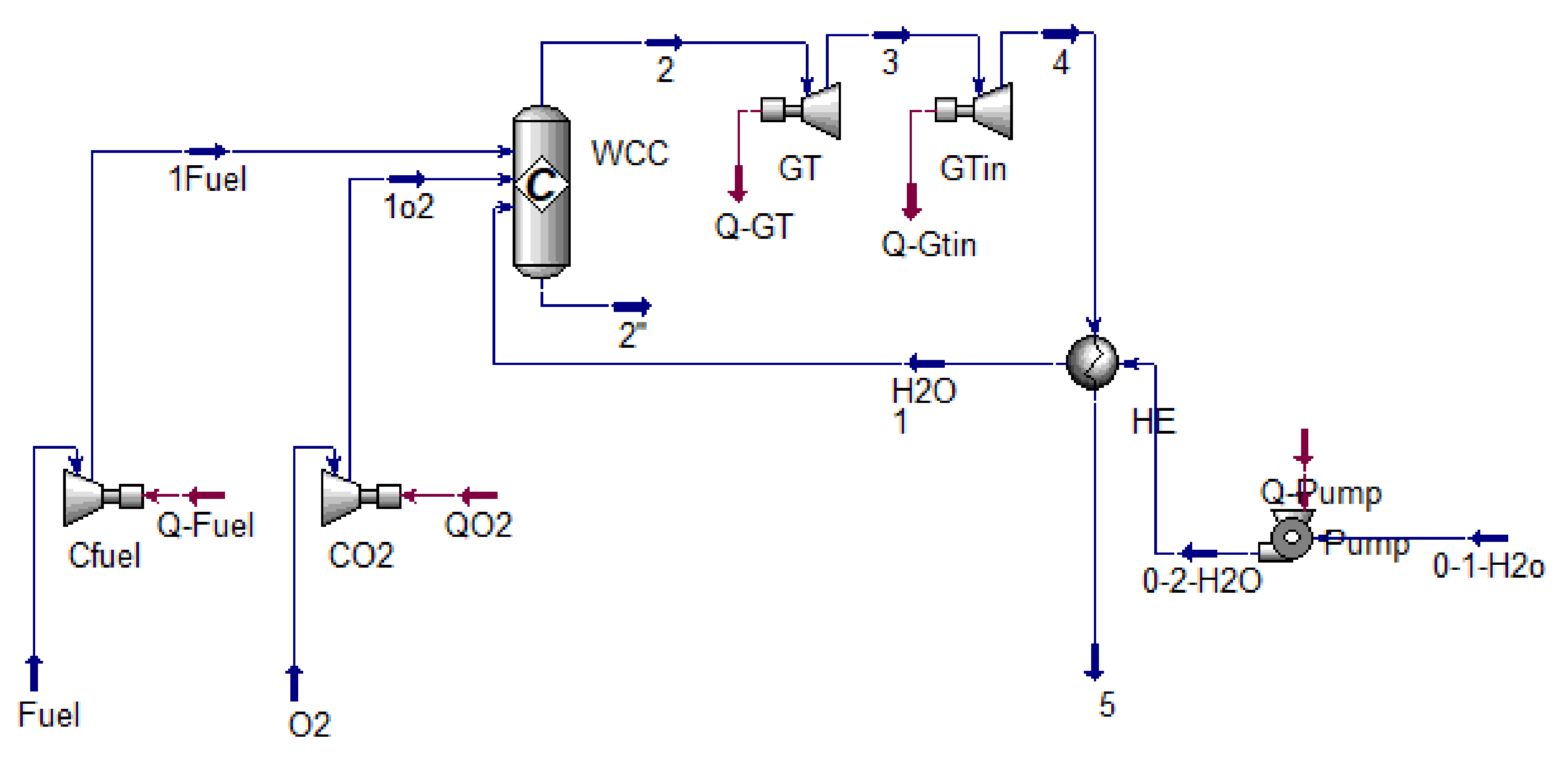
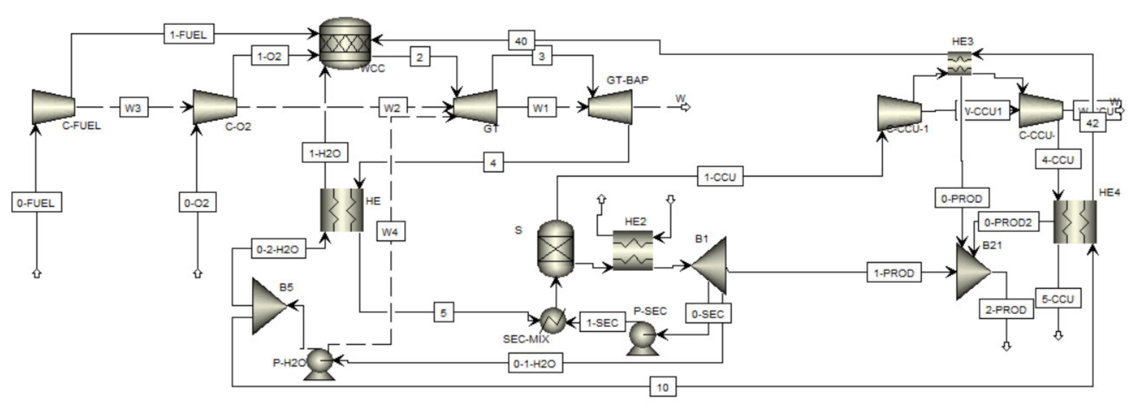
2. Thermodynamic Cycle Considered in Three Software

2.1. Modeling and Simulation of Thermodynamic Cycles

The use of thermodynamic simulation software can strongly support designing, monitoring, and optimizing CCUS processes as the new solutions for existing and planned to build power plants.

Different perspectives of modeling has been created by Aspen Plus, such as steam power plant [41], predicting emissions of NO and N₂O from coal combustion [42], catalytic coal gasification infixed beds [43], biomass gasification in fluidized bed reactor [44], and in combined heat and power (CHP) biomass bubbling fluidized bed gasification unit coupled with an internal combustion engine (ICE) [45]. Ebsilon^®Professional is a simulation software designed for performing simulations of processes in thermodynamic cycles, as well as steady-state and quasi dynamic simulations [46,47,48,49]. The Ebsilon library has an extensive number of components, useful for efficient calculations [49]. By placing the components in the system, a system of equations is generated based on mass and energy balance depending upon the component, which is solved by the Gauss–Seidel method. The iteration ends when the convergence criterion of 10-9 is reached for pressure, flow, and enthalpy variables [50]. Aspen HYSYS is defined as an industry-leading process modeling tool for conceptual study, strategic planning, management of asset, maximization and operational testing for gas processing, petroleum refining, oil and gas production, and air separation industries. Although HYSYS is mainly useful for oil and gas process industry, it is developed for various industries as follows [51]: ethanol plant; petroleum industry; heavy chemical industry; natural gas process plant; petrochemical industry; synthesis gas production; acid gas sweetening with DEA (Diethanolamine); biodiesel plant, etc. A comparison of units in Aspen Plus, Aspen HYSYS, and EBSILON is presented in

Table 1. Comparison of units in Aspen Plus, Aspen HYSYS, and EBSILON.

Unit Operation	Aspen Plus	Aspen HYSYS	EBSILON
Stream mixing	Mixer	Mixer	Simple mixer
Component splitter	Sep, Sep2	Component Splitter	Simple splitter
Decanter	Decanter	3-Phase Separator	Selective splitter
Piping	Pipe, Pipeline	Pipe Segment, Compressible Gas Pipe	Pipe
Valves and fittings	Valve	Valve, Tee, Relief Valve	Valve
Equilibrium reactor	REquil	Equilibrium Reactor	Combustion chamber
Gibbs reactor	RGibbs	Gibbs Reactor	Gibbs reactor
Heat exchanger	HeatX, HxFlux, Hetran, HTRI-Xist	Heat Exchanger	Heat exchanger
Compressor	Compr, MCompr	Compressor	Compressor
Turbine	Compr, MCompr	Expander	Gas expander
Pump	Pump	Pump	Pump

.

Differences and similarities of thermodynamic parameters for the three used software including Aspen Hysys, Plus, and Ebsilon are indicated in Table 2. Crucial parameters for thermodynamic is its efficiency, which depend from many issues, but one of the important is model of fluid. The net system efficiency of the system was calculated according to the formula:

$${\eta }_{net}=\frac{N_t-N_{C-fuel}-N_{C-O_2}-N_{P-H_{2}O}-N_{CCU}-N_{p-SEC}}{{\dot{Q}}_{CC}}$$

(1)

where:

• $N_t$—combined turbine power on the shaft in [kW],
• $N_{C-fuel}$—power for fuel compressor in [kW],
• $N_{C-O_2}$—power for oxygen compressor in [kW],
• $N_{P-H_{2}O}$—power for water pump PH₂O in [kW],
• $N_{P-SEC}$—power for water pump PSEC supplying SEC in [kW],
• $N_{CCU}$—combined power for CO₂ capture unit compressors [kW],
• ${\dot{Q}}_{CC}$—chemical energy rate of combustion in [kW].

Important is also power for own needs as a sum:

$$N_{CP}=N_{C-fuel}+N_{C-O_2}+N_{P-H_{2}O}+N_{P-SEC}+N_{CCU}$$

(2)

According this equation, the powers depend from thermodynamic model of fluid which is possible to describe the real gas equation in a more precise form, which takes the form of the Peng–Robinson gas model:

$$p=\frac{\tilde{R}T}{v_M-b}-\frac{a{\alpha }_m}{v_M^2+2b{v}_M-b^2},$$

(3)

where: $\tilde{R}$—universal gas constant, $v_M$—molar volume and

$$a=\frac{0.4572{\tilde{R}}^2{T}_{cr\left(m\right)}^2}{p_{cr\left(m\right)}}$$

(4)

where: $p_{cr\left(m\right)}$—critical pressure, $T_{cr\left(m\right)}$—critical temperature. Another constant is:

$$b=\frac{0.0778\tilde{R}{T}_{cr\left(m\right)}}{p_{cr\left(m\right)}}$$

(5)

and the last constant from the Formula (3) is expressed as:

$${\alpha }_m={\left(1+{\xi }_m\left(1-T_{r\left(m\right)}^{0.5}\right)\right)}^2$$

(6)

assuming that the reduced temperature $T_{r\left(m\right)}$ expresses the ratio:

$$T_{r\left(m\right)}=\frac{T}{T_{cr\left(m\right)}}$$

(7)

and

$${\xi }_m=0.37464+1.54226{\omega }_m-0.26992{\omega }_m^2$$

(8)

where ${\omega }_m$ is the material constant expressing the molecular non-sphericity (centrality) of the particles. For example, for noble gases such as argon, krypton, neon, and xenon ${\omega }_m=0$. It should be also mentioned that ${\omega }_m$ is determined for $T_{r\left(m\right)}=0.7$ and can be determined by the relationship:

$${\omega }_m=-{\log }_{10}\left(p_{r\left(m\right)}^{sat}\right)-1$$

(9)

where $p_{r\left(m\right)}^{sat}$ is the reduced evaporation pressure expressed as the relationship:

$$p_{r\left(m\right)}^{sat}=\frac{p_{sat\left(m\right)}}{p_{cr\left(m\right)}}$$

(10)

where $p_{sat\left(m\right)}$ is the saturation pressure (evaporation) for $T_{r\left(m\right)}=0.7$.

Although Peng-Robinson as a thermodynamic model is used for both Aspen Hysys and Plus, thermodynamic tables for steam and Peng-Robinson for another working fluid are used in Ebsilon.

Table 2. Differences and similarities for calculations.

Parameter	Symbol	Unit
Thermodynamic model	Peng-Robinson	-	Thermodynamics tables for steam and Peng-Robinson for another working fluid
Net efficiency	η_net	-	$\frac{N_t-N_{C-fuel}-N_{C-O_2}-N_{P-H_{2}O}-N_{CCU}-N_{p-SEC}}{{\dot{Q}}_{CC}}$
Gross efficiency	ηg	-	${\eta }_g=\frac{N_t}{{\dot{Q}}_{CC}}$
NOx production	NO and NO2	-	Without NOx production calculation in Ebsilon software
Chemical energy rate	${\dot{Q}}_{CC}$	kW	${\dot{Q}}_{CC}={\dot{m}}_{fuel}LHV$
Reactions	combustion	-	Defined and could be modified

Table 2. Differences and similarities for calculations.

Parameter	Symbol	Unit
Thermodynamic model	Peng-Robinson	-	Thermodynamics tables for steam and Peng-Robinson for another working fluid
Net efficiency	η_net	-	$\frac{N_t-N_{C-fuel}-N_{C-O_2}-N_{P-H_{2}O}-N_{CCU}-N_{p-SEC}}{{\dot{Q}}_{CC}}$
Gross efficiency	ηg	-	${\eta }_g=\frac{N_t}{{\dot{Q}}_{CC}}$
NOx production	NO and NO2	-	Without NOx production calculation in Ebsilon software
Chemical energy rate	${\dot{Q}}_{CC}$	kW	${\dot{Q}}_{CC}={\dot{m}}_{fuel}LHV$
Reactions	combustion	-	Defined and could be modified

It should be underscored that the specific enthalpy of the fluid h = h(p;T;Y_(k)) is determined at the characteristic points by the thermodynamic table and depends on thermodynamic parameters, such as temperature T, pressure p, and specific components within the mixture of air and exhaust gases Y_(k); k = N₂,…, Ar [52,53]. Another difference can be tangible in NO_x production so that Aspen Hysys and Plus calculate NO_x production including NO and NO₂, whilst it is not estimated in Ebsilon. In addition, reactions used in wet combustion chamber need to be defined in properties tab (Reaction’s part) in Aspen Hysys. As it can be vividly seen, the method of calculating net efficiency, gross efficiency, and chemical energy rate is the same for three used software.

2.2. Thermodynamic Cycle

The thermodynamic cycle of the gas–steam turbine system is represented in Figure 1. The gas–steam turbine system consists of two gas–steam expanders, i.e., the gas–steam turbine (GT) part and the low-pressure gas–steam turbine below ambient pressure (GT_bap) with power generators (G~), the fuel compressor (C_fuel), the oxygen compressor (C_O2), the water pump (P_H2O), the heat exchanger (HE) for regenerative water heating, and the wet combustion chamber (WCC). The working fluid in the cycle is the gas–steam—a mixture of water vapor (H₂O) and carbon dioxide (CO₂). As observed in Figure 1, after increasing the pressure of selected fuel (methane and mixture 1) and O₂ in their related compressor, they are fed to a wet combustion chamber. Wet combustion chamber combusts selected fuels in the presence of oxygen O₂ to produce hot steam and carbon dioxide. Using the recycled water leads hot steam and carbon dioxide to cool within the wet combustion chamber to the desired temperature of a gas turbine. GT and GT_bap are used to decrease high-pressure (10 bar) working fluid (water vapor and carbon dioxide) to below ambient pressure (0.078 bar). A heat exchanger is not only simulated to achieve the cooled steam but also increases the temperature of water.

2.3. Assumptions for Cycle Modeling

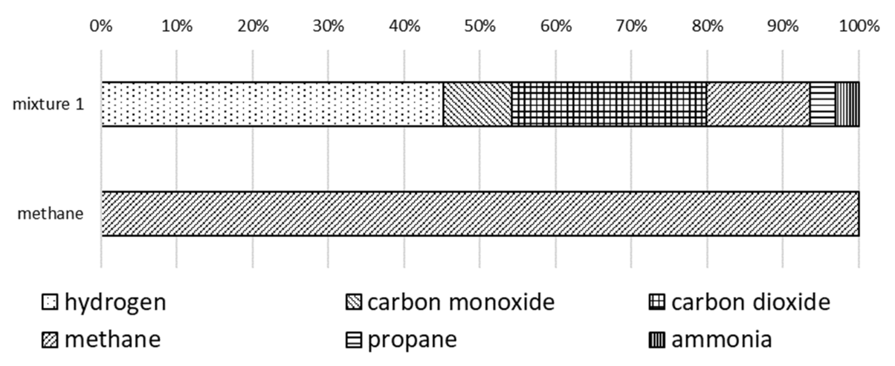
Assumptions for the thermodynamic cycle, internal efficiency, and mechanical efficiency are illustrated in

Table 3. Assumptions for the thermodynamic cycle calculation using Aspen HYSYS, Aspen Plus, and Ebsilon.

Parameters		Symbol	Unit	Value
Mass flow of exhaust gas at the outlet from combustion chamber WCC		m2	g/s	100
Air-fuel ratio in WCC		λ	-	1 (stoichiometric)
Pressure before GT		p2	bar	10
Pressure after GT		p3	bar	1
Pressure after GTbap		p4	bar	0.078
Water pressure to WCC		p1-H2O	bar	300
Temperature exhaust after WCC (before GT)		t2	°C	1100 (1100 and variable in Ebsilon)
Initial water temperature (before PH2O pump)		t0-1-H2O	°C	15
Initial fuel temperature		tfuel	°C	15
Initial oxygen temperature		tO2	°C	15
Initial fuel pressure (before Cfuel compressor)		p0-fuel	bar	1
Initial oxygen pressure (before CO2 compressor)		p0-O2	bar	1
Fuel to WCC pressure loss factor		δfuel	-	0.05
Oxygen to WCC pressure loss factor		δO2	-	0.05
Oxygen purity			%	100
Fuel mass flow	methane	${\dot{m}}_{fuel}$	g/s	6.72
	Mixture—syngas	${\dot{m}}_{fuel}$	g/s	18.00
Temperature exhaust after WCC (before GT)	Variable temperature in point 1H2O (118.45; 131.84 and 125.1 °C)	$t_2$ = const	°C	1100
	Constant temperature in point 1H2O (125.1 °C)	$t_2$ = var	°C	1100 1073 for mixture, 1091 for methane in Ebsilon
CO2 fraction from combustion of methane	Methane	$X_{C{O}_2}=const$	mol%	8.47
	Mixture	$X_{C{O}_2}=var$	mol%	11.75 11.73 in Ebsilon
Water temperature before combustion chamber	Variable temperature exhaust after WCC	$t_{1 H_{2}O}$ = const	°C	125.1
	Constant temperature exhaust after WCC	$t_{1 H_{2}O}$ = var	°C	149.02 for mixture and 131.84 for methane in Ebsilon

,

Table 4. Assumed internal efficiency (adiabatic for Hysys and isentropic for Aspen Plus and Ebsilon).

Internal Efficiency	Symbol	Unit	Value
Turbine GT	ηiGT	-	0.89
Turbine GTbap	ηiGT-bap	-	0.89
Fuel compressor Cfuel	ηiC-fuel	-	0.87
Oxygen compressor CO2	ηiC-O2	-	0.87
Water pump PH2O	ηiP-H2O	-	0.43

and

Table 5. Assumed mechanical efficiency—for Aspen Hysys it is impossible to change value.

Internal Efficiency	Symbol	Unit	Aspen HYSYS	Aspen Plus/EBSILON
Turbine GT	ηmGT	-	1	0.99
Turbine GTbap	ηmGT-bap	-	1	0.99
Fuel compressor Cfuel	ηmC-fuel	-	1	0.99
Oxygen compressor CO2	ηmC-O2	-	1	0.99
Water pump PH2O	ηmP-H2O	-	1	0.99

. It can be noticed that the temperature of exhaust gas after WCC (before GT) is 1100 °C in Aspen Hysys and Plus and Ebsilon for (Ebsilon t₂ = const), while for Ebsilon t₂ = var is 1073 °C for methane and 1091 °C for mixture 1, respectively. These temperatures (namely 1100 °C in Aspen Plus and Aspen Hysys, and 1091 °C and 1073 °C) in front of the turbine were achieved by assuming a constant temperature of water feeding the combustion chamber, namely t₁H₂O = const = 125.1 °C. In addition, when the exhaust temperature after WCC is constant (t₂ = 1100 °C), water temperature before the combustion chamber is variable, respectively, 149.02 °C in Ebsilon with mixture 1, 131.84 °C in Ebsilon with methane, and 125.1 °C for both Aspen Hysys and Plus. Heat efficiency of the combustion chamber in Aspen Plus and Aspen Hysys is 99.9%. The rest of the assumptions for the three used software is the same.

2.4. Fuels

Syngas fuels produced from gasification are expected to be of different compositions, mainly due to inherent variability of sewage sludge composition, as reported by Werle and Wilk [54]. Therefore, two types of fuel were selected for the analysis, and compositions are presented in Figure 5. The first one is the syngas mixture which contains CO (9.09%_mol); CO₂ (25.61%_mol); CH₄ (13.64%_mol); C₃H₈ (3.39%_mol); H₂ (45.16%_mol); and NH₃ (3.10%_mol). However, the mass fractions of species for Aspen Plus and Aspen Hysys was introduced as data, namely CO (13.31%_mass); CO₂ (59.31%_mass); CH₄ (11.46%_mass); C₃H₈ (8.03%_mass); H₂ (5.10%_mass); and NH₃ (2.79%_mass). Selected compositions of the producer gas are well within the ranges of values are reported by Achweizer et al. [55] or Akkache et al. [56]. Methane fuel is added for comparison purposes. The compositions of selected fuels, including methane and mixture (syngas), are shown in Figure 5.

The values of LHV for mixture 1 and methane at 15 °C and 1 atm are presented in

Table 6. LHV based on ISO 6976:1995(E) for gas mixtures, value at 15 °C and 1 atm derived from Aspen and Ebsilon.

Software	LHV, MJ/kg
	Syngas—Mixture	Methane
Aspen HYSYS and Aspen PLUS	17.079	50.035
Ebsilon	17.081	50.015

. It is noteworthy that Ebsilon uses empirical formulae based on elementary analysis, whereas LHV used for both Aspen Hysys and Plus are the same. Syngas is produced by gasifying sewage sludge.

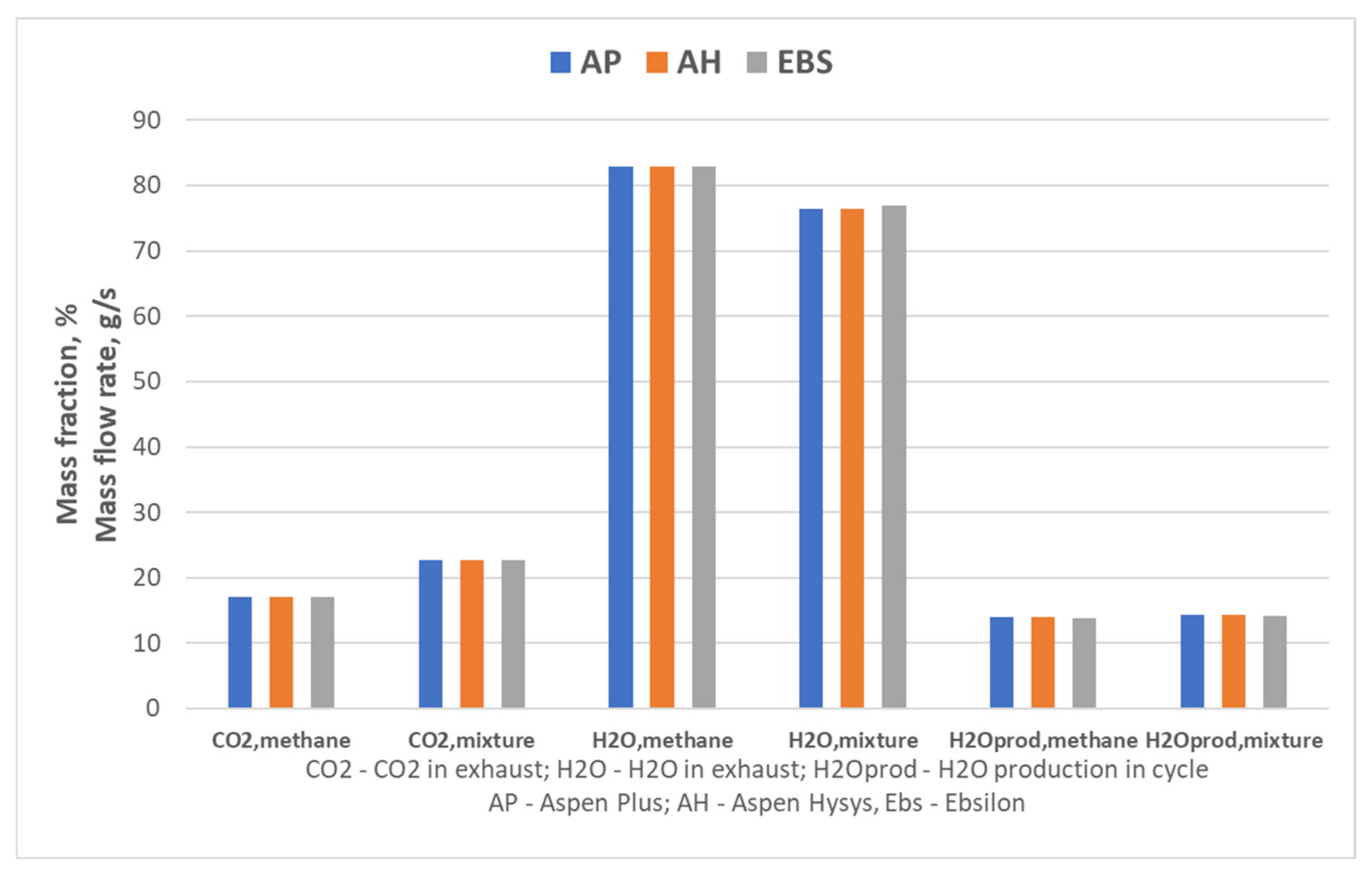
3. Results and Comparison

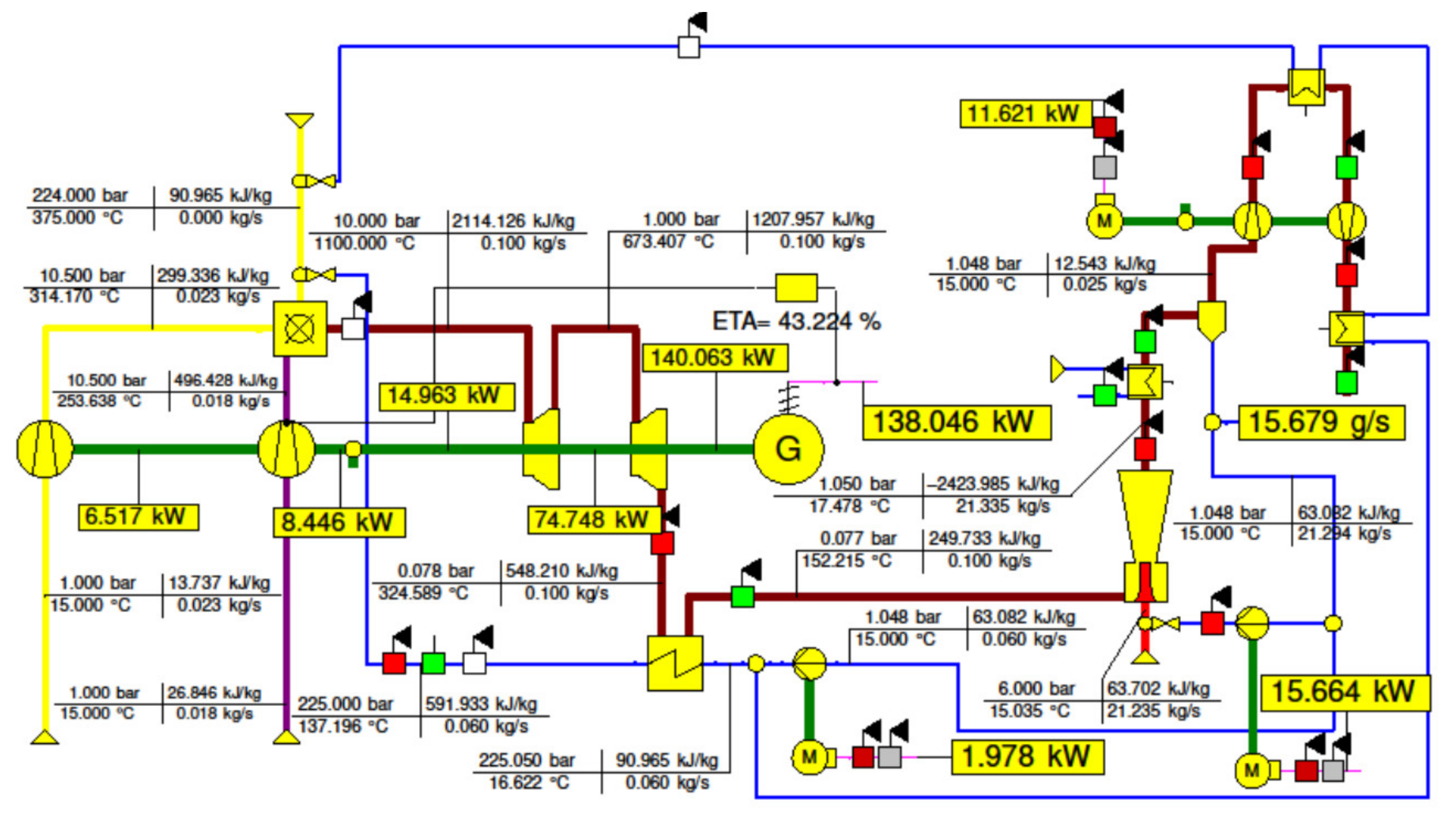
The most important nodal point results are presented in Section 3.1, while Section 3.2 refers to the efficiency results and Section 3.3 deals with the combustion of ammonia to various nitrogen compounds.

3.1. Nodal Points

Cycle nodal points for mixture (syngas) and methane are depicted in

Table 7. Cycle nodal points on basis of syngas—mixture of gases as a fuel.

Parameter	Case	Unit	Value
Node Designation	-	-	0 Fuel	1 Fuel	0 O2	1 O2	0 1-H2O	0 2-H2O	1 H2O	2	3	4	5
	Aspen Hysys	g/s	18.0	18.0	23.2	23.2	58.8	58.8	58.8	100	100	100	100
Mass flow	Aspen Plus
$\dot{m}$	Ebsilon $t_2$ = var				22.4	22.4	59.6	59.6	59.6
	Ebsilon $t_2$ = const
O2 fraction $(X_{O_2})$	Aspen Hysys	mol%	-	-	100	100	-	-	-
	Aspen Plus		-	-			-	-	-
	Ebsilon $t_2$ = var		-	-			-	-	-	0.00	0.00	0.00	0.00
	Ebsilon $t_2$ = const		-	-			-	-	-
CO2 fraction ($X_{C{O}_2})$	Aspen Hysys		-	-	-	-	-	-	-	11.75	11.75	11.75	11.75
	Aspen Plus	mol%	-	-	-	-	-	-	-
	Ebsilon $t_2$ = var		-	-	-	-	-	-	-	11.73	11.73	11.73	11.73
	Ebsilon $t_2$ = const		-	-	-	-	-	-	-
H2O fraction ($X_{H_{2}O})$	Aspen Hysys		-	-	-	-	100	100	100	87.63	87.63	87.63	87.63
	Aspen Plus	mol%	-	-	-	-
	Ebsilon $t_2$ = var		-	-	-	-
	Ebsilon $t_2$ = const		-	-	-	-				87.96	87.96	87.96	87.96
	Aspen Hysys		-	-	-	-	-	-	-
NO fraction (N2 in Ebsilon) ($X_{NO})$	Aspen Plus	mol%	-	-	-	-	-	-	-	0.62	0.62	0.62	0.62
	Ebsilon $t_2$ = var		-	-	-	-	-	-	-
	Ebsilon $t_2$ = const		-	-	-	-	-	-	-	0.31	0.31	0.31	0.31
	Aspen Hysys		15	255.6		314.8	15	25.11	125.11		672.5	324.7	178.6
Temperature ($t)$	Aspen Plus	°C		253.33	15	315.08				1100	672.51	323.64	183.58
	Ebsilon $t_2$ = const			252.38		314.17		24.98	149.02		673.58	324.86	147.3
	Ebsilon $t_2$ = var								125.11	1073	652.98	310.38	167.64
	Aspen Hysys
Pressure $\left(p\right)$	Aspen Plus	bar	1	10.5	1	10.5	1	300	300	10	1	0.078	0.078
	Ebsilon $t_2$ = var												0.077
	Ebsilon $t_2$ = const

and

Table 8. Cycle nodal points on basis of methane.

	Symbol	Unit	Value
Node Designation	-	-	0 Fuel	1 Fuel	0 O2	1 O2	0 1-H2O	0 2-H2O	1 H2O	2	3	4	5
	Aspen Hysys
Mass flow	Aspen Plus	g/s	6.72	6.72	26.80	26.80	66.48	66.48	66.48	100	100	100	100
$\left(\dot{m}\right)$	Ebsilon $t_2$ = var
	Ebsilon $t_2$. = const
	Aspen Hysys
O2 fraction	Aspen Plus	mol%	-	-	100	100	-	-	-	0.00	0.00	0.00	0.00
$(X_{O_2})$	Ebsilon $t_2$ = var
	Ebsilon $t_2$ = const
	Aspen Hysys
CO2 fraction	Aspen Plus	mol%	-	-	-	-	-	-	-	8.47	8.47	8.47	8.47
($X_{C{O}_2})$	Ebsilon $t_2$ = var
	Ebsilon $t_2$ = const
	Aspen Hysys						100	100	100	91.53
H2O fraction	Aspen Plus	mol%	-	-	-	-					91.53	91.53	91.53
($X_{H_{2}O})$	Ebsilon $t_2$ = var
	Ebsilon $t_2$ = const
	Aspen Hysys			225.39		314.8			125.11		667.3	318.4	158.6
Temperature ($t)$	Aspen Plus	°C	15		15	315.08	15	25.11		1100	669.51	318.99	165.82
	Ebsilon $t_2$ = const			224.63		314.17		24.98	131.84		670.49	320.01	155.65
	Ebsilon $t_2$ = var								125.11	1091	663.9	315.35	161.47
	Aspen Hysys
Pressure $\left(p\right)$	Aspen Plus	bar	1	10.5	1	10.5	1	300	300	10	1	0.078	0.078
	Ebsilon $t_2$ = var
	Ebsilon $t_2$ = const												0.077

, respectively. Having studied the data from Table 7, it can be considered that mass flow of mixture (syngas), O₂, and H₂O are 18 (g/s), 23.19 (g/s), and 58.80 (g/s) in Aspen Hysys and Plus, whilst these values in Ebsilon are 18 (g/s), 22.84 (g/s), and 59.164 (g/s), respectively. It is noticeable that simulation in Ebsilon was performed for two values of t₂ (temperature after WCC), as mentioned in Table 3. The temperature after compressor of fuel (syngas) is 255.6 °C, 253.33 °C, and 252.38 °C and after compressor of O₂ is 314.8 °C, 315.08 °C, and 314.17 °C in Aspen Hysys, Plus, and Ebsilon, respectively. Other differences can be observed in temperature before and after the heat exchanger. More accurately, temperature before heat exchanger is 25.11 °C for both simulation in Apen Hysys and Plus, whereas its value is 24.98 °C in Ebsilon. These temperatures are obtained by increasing the pressure in the pump.

As the same way, the temperature after heat exchanger is 125.11 °C was the same for both simulations in Apen Hysys and Plus, while it is 125.11 °C and 149.02 °C for mixture 1, 125.11 °C and 131.84 °C for methane when t₂ = var and t₂ = const in Ebsilon, respectively. In addition, CO₂, H₂O, and NO (N₂ in Ebsilon) result from combustion in a wet combustion chamber. As seen in Table 7, mole fraction of CO₂ is 11.75 and 11.73 in Aspen Hysys, Plus, and Ebsilon, respectively. Moreover, mole fraction of H₂O is 87.63 and 87.98 for mentioned software, respectively. The most important difference in arising composition is in the type of NO_x, so that there is NO (0.62) in Aspen Hysys and Plus, whereas N₂ (0.32) is created in Ebsilon. Although it is assumed that the temperature after wet combustion chamber is 1100 °C for Aspen Hysys, Plus, and Ebsilon, a different temperature (1073 °C) after WCC was simulated in Ebsilon. Results show that the maximum temperature of exhaust gases after the heat exchanger results from simulation of Aspen Plus and its value is 183.58 °C whereas the minimum one (147.3 °C) belongs to the simulation using Ebsilon (t₂ = const).

As it can be observed that the difference in temperature (324.7 °C in Hysys, 323.64 °C in Plus, and 324.82 °C in Ebsilon) before heat exchanger for gas–steam is less than 0.4%, the type of heat exchanger plays an indispensable role in regard to the value of cooled gas–steam (exhaust gases). In addition, pressure drop of heat exchanger is zero in Aspen Hysys and Plus, but a pressure drop is not constant in Ebsilon (pressure differences between point 4 and 5). Moreover, decreasing the temperature after wet combustion chamber leads to increasing the temperature of cooled gas–steam (t₅), so that approximately a 12% increase in temperature of steam after heat exchanger results from decreasing the temperature after WCC from 1100 to 1073 °C.

Cycle nodal points for methane are indicated in Table 8. Mass flow of fuel, O₂, and H₂O are the same for used software and its value is 6.72 (g/s), 26.80 (g/s), and 66.48 (g/s), respectively. Although the temperature of water that was fed to WCC is 125.11 °C, this value indicates for simulation various temperature in combustion chamber (t₂ = 1091 °C) in Ebsilon and (t₂ = 1100 °C) in Aspen Plus and Aspen Hysys. To obtain the same temperature in combustion chamber in simulation using a Ebsilon, we need to increase temperature to 131.84 °C. Moreover, a decrease (0.82%) in the temperature of exhaust gases after WCC from 1100 °C to 1091 °C results in an increase (3.6%) in temperature of cooled gas–steam after heat exchanger from 155.65 °C to 161.47 °C in Ebsilon.

As a result, changing the type of fuels leads to a change in the compositions of exhaust gases and temperature after a heat exchanger. For example, approximately 88% and 92% mole fraction of H₂O result from mixture 1 (syngas) and methane, respectively. Furthermore, using a mixture of gases as a fuel and methane result in creating approximately 12% and 8% mole fraction of CO₂. Moreover, the average temperature (among three software) after the heat exchanger is 169.3 °C for mixture and 160 °C for methane.

3.2. Efficiency and Summarized Effects

Summarized results for two fuels (mixture 1 and methane) in three used software including Aspen Hysys, Plus, and Ebsilon are illustrated in

Table 9. Effect of different fuels.

Parameter	Symbol	Unit	Mixture 1 (Syngas)	Methane
Temperature at the WCC outlet	$t_2$= var	°C	1073	1091
	$t_2$ = const	°C	1100	1100
Fuel mass flow (${\dot{m}}_{1-fuel}$)	Aspen Hysys	g/s	18.00	6.72
	Aspen Plus
	Ebsilon $t_2$ = var
	Ebsilon $t_2$ = const
Oxygen mass flow $({\dot{m}}_{1-O_2}$)	Aspen Hysys	g/s	23.2	26.8
	Aspen Plus
	Ebsilon $t_2$ = var		22.4
	Ebsilon $t_2$ = const
Water mass flow $({\dot{m}}_{1-H_{2}O})$	Aspen Hysys	g/s	58.8	66.48
	Aspen Plus
	Ebsilon $t_2$ = var		59.6
	Ebsilon $t_2$ = const
Exhaust temperature after HE $(t_5)$	Aspen Hysys	°C	178.60	161.10
	Aspen Plus		183.58	165.82
	Ebsilon $t_2$ = var		167.64	161.47
	Ebsilon $t_2$ = const		147.3	155.65
Turbine power GT $(N_{GT})$	Aspen Hysys	kW	88.73	92.93
	Aspen Plus		89.30	93.20
	Ebsilon $t_2$ = var		87.67	92.65
	Ebsilon $t_2$ = const		89.53	93.26
Turbine power GTbap   $\left(N_{GT-bap}\right)$	Aspen Hysys	kW	65.64	68.49
	Aspen Plus		64.9	67.52
	Ebsilon $t_2$ = var		63.69	67.11
	Ebsilon $t_2$ = const		65.20	67.63
Combined turbines gross power $(N_t)$	Aspen Hysys	kW	154.37	161.42
	Aspen Plus		154.20	160.72
	Ebsilon $t_2$ = var		151.36	159.76
	Ebsilon $t_2$ = const		154.72	160.89
Power for own needs $(N_{cp})$	Aspen Hysys	kW	19.12	15.75
	Aspen Plus		19.30	16
	Ebsilon $t_2$ = var		18.94	15.954
	Ebsilon $t_2$ = const			15.954
Chemical energy rate of combustion ${\dot{Q}}_{cc}$	Aspen Hysys	kW	307.42	336.23
	Aspen Plus
	Ebsilon $t_2$ = var		307.45	336.1
	Ebsilon $t_2$ = const
Net efficiency $({\eta }_{net})$	Aspen Hysys	%	44.00	43.32
	Aspen Plus		43.88	43.05
	Ebsilon $t_2$ = var		43.07	42.8
	Ebsilon $t_2$ = const		44.16	43.12
Gross efficiency $({\eta }_g)$	Aspen Hysys	%	50.21	48.01
	Aspen Plus		50.16	47.81
	Ebsilon $t_2$ = var		49.23	47.55
	Ebsilon $t_2$ = const		50.32	47.86

. The mass flow rate after WCC is 100 g/s for the three mentioned software. The gross power of turbines for mixture is 154.37 kW, 154.20 kW, 154.72 kW (t₂ = const), and 151.36 kW (t₂ = var) in Aspen Hysys, Plus, and Ebsilon, respectively. It can be observed that less than a 0.34% difference was obtained among three software, when t₂ is 1073 °C or 1100 °C. On the other hand, for methane, these values are 161.42 kW, 160.72 kW, 160.89 kW (t₂ = const), and 159.76 kW (t₂ = var) for the mentioned software, respectively. The results show that, at the same assumption, changing the type of fuels from mixture 1 to methane leads the gross power output of turbines to increase approximately by 4% in Aspen Hysys, Plus and Ebsilon (t₂ = const) and approximately by 5% in Ebsilon (t₂ = var).

According to calculation of chemical energy rate of combustion Q_cc mentioned in Table 2 and Table 9, this value in used software is approximately 307 kW and 336 kW for mixture 1 and methane, respectively. The results represent that the net efficiency of the system is 44%, 43.8%, 44.16%, and 43.07% for mixture 1 in Aspen Hysys, Plus, Ebsilon (including t₂ = const and t₂ = variable), respectively. These values are 43.32%, 43.05%, 43.12%, and 42.8% for methane for the mentioned software, respectively. It can be found from the results of Aspen Hysys, Plus, and Ebsilon (t₂ = const) that, at the same assumption, changing fuels from methane to mixture results in rising the net efficiency of system from 1.5 to 2.4%.

The main source of the difference in the results obtained in Section 3.1 and Section 3.2 is the fact that the specific heat was determined differently. This becomes apparent in the temperature results after pumps, compressors, and expanders.

3.3. N₂, NO, N₂O and NO₂ Formation and Influence on Temperature

This subsection is intended to indicate the effect of the ammonia combustion reaction on the temperature in the combustion chamber. Due to the fact that Ebsilon is mainly adapted to flow analyses with less flexibility in setting combustion data, this subsection is mainly based on results from Aspen Plus and Aspen Hysys. General chemical reactions in ammonia combustion are as follows:

$$4{\mathrm{NH}}_3+3{\mathrm{O}}_2\to 2{\mathrm{N}}_2+6{\mathrm{H}}_2\mathrm{O}$$

(11)

$$4{\mathrm{NH}}_3+5{\mathrm{O}}_2\to 4\mathrm{NO}+6{\mathrm{H}}_2\mathrm{O}$$

(12)

$$4{\mathrm{NH}}_3+7{\mathrm{O}}_2\to 4{\mathrm{NO}}_2+6{\mathrm{H}}_2\mathrm{O}$$

(13)

$$2{\mathrm{NH}}_3+2{\mathrm{O}}_2\to {\mathrm{N}}_2\mathrm{O}+3{\mathrm{H}}_2\mathrm{O}$$

(14)

In Ebsilon, the basic reaction is the conversion of ammonia to nitrogen according to reaction (11). Aspen Plus, on the other hand, assigns the basic reaction to the conversion of ammonia to nitric oxide according to stoichiometric Equation (12), by default. However, due to the fact that different results are obtained in Table 7 and Table 9, it was worthwhile to trace the other possibilities for the conversion of ammonia in the presence of oxygen and hence a set of (14) equations.

HYSYS calculates and displays the heat of reactions in the reaction heat cell.

Table 10. Reaction heat for different reactions obtained by Hysys.

Reactions	Heat of Reaction *, kJ/kgmol
$4{\mathrm{NH}}_3+3{\mathrm{O}}_2\to 2{\mathrm{N}}_2+6{\mathrm{H}}_2\mathrm{O}$	−3.2 × 105
$4{\mathrm{NH}}_3+5{\mathrm{O}}_2\to 4\mathrm{NO}+6{\mathrm{H}}_2\mathrm{O}$	−2.3 × 105
$4{\mathrm{NH}}_3+7{\mathrm{O}}_2\to 4{\mathrm{NO}}_2+6{\mathrm{H}}_2\mathrm{O}$	−2.8 × 105
$2{\mathrm{NH}}_3+2{\mathrm{O}}_2\to {\mathrm{N}}_2\mathrm{O}+3{\mathrm{H}}_2\mathrm{O}$	−2.8 × 105

* at 25 °C.

depicts the reaction heat of different mentioned reactions. In this case, all of the reaction heat cells are negative, indicating that the reaction produces heat (exothermic). In thermodynamics, the term exothermic process describes a process or reaction that releases energy from the system to its surroundings, usually in the form of heat, but also in a form of light (e.g., a spark, flame, or flash), electricity (e.g., a battery), or sound (e.g., explosion heard when burning hydrogen). So, reactions 11 to 14 release 3.2 × 10⁵ (kJ/kgmol), 2.3 × 10⁵ (kJ/kgmol), 2.8 × 10⁵ (kJ/kgmol), and 2.8 × 10⁵ (kJ/kgmol), respectively. It can be understood that if all of these reactions could occur, reaction 11 releases the highest value of energy. This would take precedence in comparison to other reactions. Meanwhile, it is assumed that, in combined reaction, including reactions of N₂, N₂O, NO, and NO₂, each reaction is with ammonia conversion factor of 0.25.

The effect of an ammonia combustion reaction on the temperature is shown in

Table 11. 18 g/s mixture 1 (syngas) with NH₃ combustion to NO, NO₂, N₂, N₂O under stoichiometric conditions (100 g/s exhaust).

Parameter	Symbol	Unit	Combined *	N2	N2O	NO	NO2
Temperature at the WCC outlet $t_2$ = var	Aspen Hysys	°C	1107	1106	1104	1100	1116
	Aspen Plus		1106	1105	1103	1100	1115
	Ebsilon		n.a.	1100	n.a.	n.a.	n.a.
Fuel mass flow (${\dot{m}}_{1-fuel}$)	Aspen Hysys	g/s	18.00
	Aspen Plus
	Ebsilon
Oxygen mass flow $({\dot{m}}_{1-O_2}$)	Aspen Hysys	g/s	23.13	22.72	22.96	23.19	23.66
	Aspen Plus		23.13	22.72	22.96	23.19	23.66
	Ebsilon		n.a.	22.4	n.a.	n.a.	n.a.
Water mass flow $({\dot{m}}_{1-H_{2}O})$	Aspen Hysys	g/s	58.86	59.28	59.04	58.80	58.33
	Aspen Plus		58.86	59.28	59.04	58.80	58.33
	Ebsilon		n.a.	59.6	n.a.	n.a.	n.a.
Exhaust temperature after HE $(t_5)$	Aspen Hysys	°C	187.9	186.1	186.3	183.60	195.00
	Aspen Plus		187.33	185.57	185.81	183.55	194.44
	Ebsilon		n.a.	147.3	n.a.	n.a.	n.a.
Turbine power GT $(N_{GT})$	Aspen Hysys	kW	89.40	89.61	89.26	89.05	89.66
	Aspen Plus		89.58	89.79	89.44	89.25	89.85
	Ebsilon		n.a.	89.53	n.a.	n.a.	n.a.
Turbine power GTbap   $\left(N_{GT-bap}\right)$	Aspen Hysys	kW	65.46	65.58	65.37	65.14	65.75
	Aspen Plus		65.23	65.35	65.13	64.92	65.53
	Ebsilon		n.a.	65.2	n.a.	n.a.	n.a.
Combined turbines gross power $(N_t)$	Aspen Hysys	kW	154.9	155.2	154.6	154.2	155.4
	Aspen Plus		154.8	155.1	154.6	154.2	155.4
	Ebsilon		n.a.	154.72	n.a.	n.a.	n.a.
Power for own needs $(N_{cp})$	Aspen Hysys	kW	19.03	18.94	18.99	19.05	19.15
	Aspen Plus		19.28	19.19	19.25	19.30	19.40
	Ebsilon		n.a.	18.94	n.a.	n.a.	n.a.
Chemical energy rate of combustion ${\dot{(Q}}_{CC})$	Aspen Hysys	kW	307.49
	Aspen Plus
	Ebsilon		307.45
Net efficiency $({\eta }_{net})$	Aspen Hysys	%	44.18	44.32	44.12	43.96	44.32
	Aspen Plus		44.08	44.21	44.01	43.86	44.22
	Ebsilon		n.a.	44.16	n.a.	n.a.	n.a.
Gross efficiency $({\eta }_g)$	Aspen Hysys	%	50.37	50.48	50.30	50.16	50.55
	Aspen Plus		50.35	50.45	50.27	50.14	50.53
	Ebsilon		n.a.	50.32	n.a.	n.a.	n.a.
N2 mass flow	Aspen Hysys	g/s	0.10	0.41	-	-	-
	Aspen Plus		0.10	0.41
	Ebsilon		n.a.	0.31
N2O mass flow	Aspen Hysys	g/s	0.16	-	0.65	-	-
	Aspen Plus		0.16		0.65
	Ebsilon		n.a.		n.a.
NO mass flow	Aspen Hysys	g/s	0.22	-	-	0.89	-
	Aspen Plus		0.22			0.89
	Ebsilon		n.a.			n.a.
NO2 mass flow	Aspen Hysys	g/s	0.34	-	-		1.36
	Aspen Plus		0.34				1.36
	Ebsilon		n.a.				n.a.

* Combined—each reaction with ammonia conversion factor of 0.25 (0.25 × 4 = 1).

. It shows the results obtained with Aspen Plus and Aspen Hysys. On the basis of the given chemical reactions and the obtained results of temperature and elemental compositions downstream of the combustion chamber, it should be concluded that the highest energy effect accompanies the formation of NO₂, followed by the formation of N₂ and N₂O, successively, and the lowest temperature is downstream of the combustion chamber after the formation of NO.

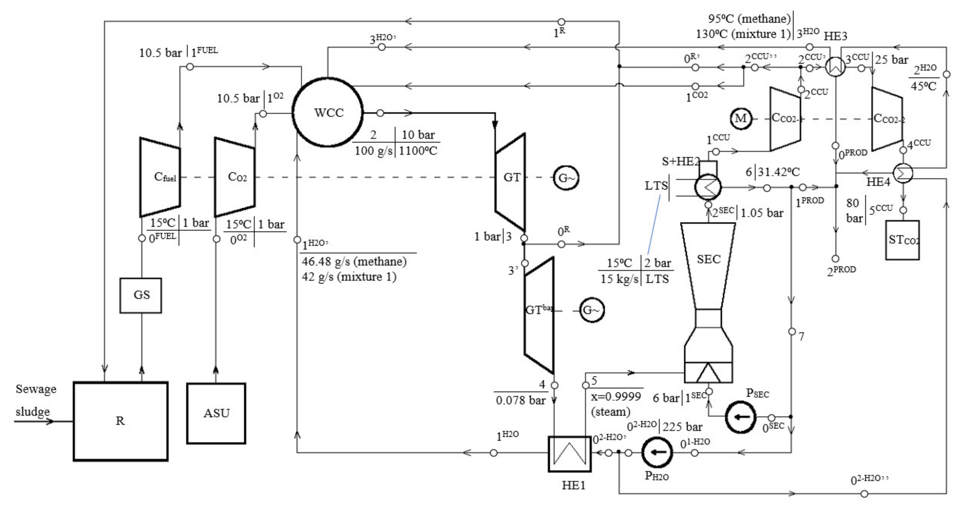
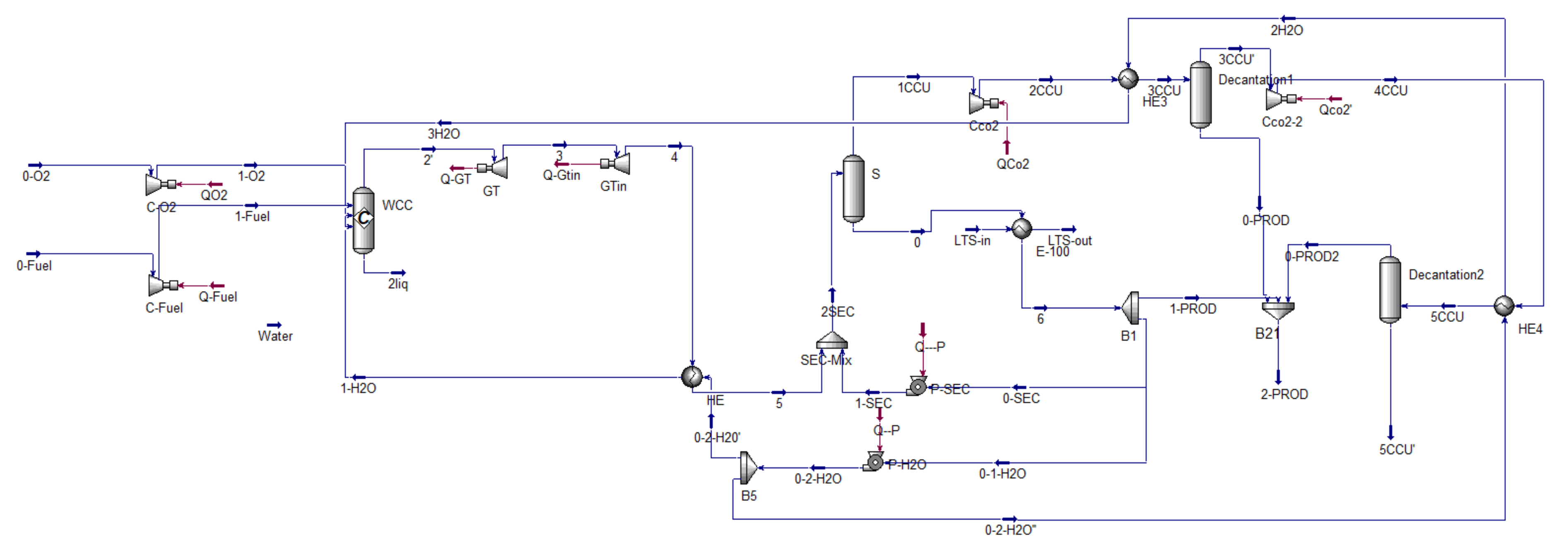
4. PFD with Spray Ejector Condenser

In Figure 6, the extended version of the “PFD0” cycle is presented, shown in the previous chapter. The developed cycle “PFD1” includes additionally fuel preparation and carbon capture storage (CCS) units. Fuel comes out from the gasifier (R) as a product of a thermochemical process transformation of supplied dry sewage sludge in the presence of a gasifying agent. The gasifying agent is released after GT with optional release from a carbon capture unit (CCU) at an ambient pressure, consisting of a mixture of steam and CO₂. The gasifying agent properties, such as content of CO₂, steam, and its temperature or pressure, can be controlled as required. An oxygen compressor (CO₂) is supplied from an air separation unit (ASU). A spray ejector condenser (SEC) sucks the exhaust from the heat exchanger 1 (HE1), while the motive fluid is supplied to SEC through the dedicated pump (PSEC).

The outlet mixture of condensed steam and moist CO₂ vapor from SEC is directed to the separator with heat exchanger 2 (S + HE2), where low temperature source (LTS) is supplied and separation of CO₂ takes place. Water from HE2 is directed to PH2O and PSEC, while excess water is discharged out of the plant. Humid CO₂ vapor from the separator is directed to the CCU whereby, after each CO₂ compressor 1 and 2 (CCO2-1 and CCO2-2), there are intercoolers heat exchangers 3 and 4 (HE3 and HE4) with decantation which are supplied with water supplied from PH2O. Water after heating in CCU is directed to WCC where it reaches supercritical conditions. A partial release of CO₂ vapor can be used as a gasifying agent to the gasifier (R) or to WCC to manipulate and obtain the desired chemical reactions pathway. CO₂ vapor is directed to CO₂ storage tank (STCO₂) or can be used for other processes, such as methanol production.

The simulation models of “PFD1” developed in different computing codes are presented in Figure 7, Figure 8 and Figure 9 (Aspen Hysys—Figure 7, Aspen Plus—Figure 8, Ebsilon—Figure 9), with most significant assumptions and calculated values in nodal points. Models do not contain the part connected with fuel preparation (gasifier and air separation unit). The main difference between models was approach to CCS part, especially with SEC modeling. The Ebsilon model (Figure 9) uses a spray ejector component, whereas other cycles define SEC operation through indirect models (direct-contact heat exchanger model, as shown in Figure 7 and Figure 8). Moreover, cycles have a different arrangement of circulating water, which is extracted from exhaust gases. Next, through various configuration systems of heat exchanger, pumps are directed to WWC or SEC. One of the differences of simulation between Aspen Hysys and Plus is to consider decantation of heat exchangers. More accurately, separators are assumed in Aspen Hysys for decantation of heat exchangers, named decantation 1 and decantation 2, as seen in Figure 7.

In addition, although five reactions are available for mixture 1 fuel as a default in Aspen Plus, there is a need to define these five reactions in Aspen Hysys.

Subsection

A power plant design based on “PFD1” presented in this paper supplied with mixture 1 syngas fuel is assumed to be the target operation configuration.

Table 12. Results for mixture 1 and methane—“PFD1”—summary table.

Parameter	Symbol	Unit	Value Aspen Plus		Value Aspen HYSYS		Value Ebsilon
Fuel type	$-$	-	Mixture 1	Methane	Mixture 1	Methane	Mixture 1	Methane
Fuel mass flow	${\dot{m}}_{1-fuel}$	g/s	16.68	6.23	16.68	6.23	16.68	6.23
Oxygen mass flow	${\dot{m}}_{1-O_2}$	g/s	21.21	24.86	21.21	24.86	20.76	24.85
Water mass flow	${\dot{m}}_{1-H_{2}O}$	g/s	62.11	68.91	62.11	68.91	62.56	68.92
CO2 mass flow in exhaust	${\dot{m}}_{2-C{O}_2}$	g/s	22.68	17.10	22.68	17.10	22.68	17.09
NO mass flow in exhaust	${\dot{m}}_{2-NO}$	g/s	0.82	-	0.82	-	-	-
Water mass flow in exhaust	${\dot{m}}_{2-H_{2}O}$	g/s	76.50	82.90	76.50	82.90	76.93	82.91
Water production	${\dot{m}}_{p-H_{2}O}$	g/s	14.38	14.00	14.38	14.00	14.226	13.876
Exhaust temperature (before regenerative HE1, after GTbap)	$t_4$	°C	322.11	317.95	321.4	317.1	288.0	283.04
Exhaust temperature (after regenerative HE1, x = 0.9999)	$t_5$	°C	41.83	41.83	38.95	39.73	38.95	39.73
Turbine power GT	$N_{GT}$	kW	90.3	94.0	91.05	95.38	86.00	89.168
Turbine power GTbap	$N_{GT-bap}$	kW	65.6	68.0	66.14	69.04	62.16	64.19
Combined turbines gross power	$N_t$	kW	155.9	162.0	157.19	164.42	148.16	153.358
Optimistic SEC Pump power consumption (x = 0 in mixing part of SEC)	$N_{P-SEC,o}$	kW	17.79	12.94	17.79	12.89	14.57	14.84
Not optimistic SEC Pump power consumption (x = 0.25 in mixing part of SEC)	$N_{P-SEC,n}$	kW	54.93	53.19	54.93	53.18
Power for own needs with optimistic SEC	$N_{cp,o}$	kW	43.61	32.49	43.59	32.62	41.22	35.612
Power for own needs with optimistic SEC	$N_{cp,no}$	kW	80.75	72.74	80.63	72.91
Chemical energy rate of combustion	${\dot{Q}}_{CC}$	kW	284.86	311.82	284.88	311.72	284.97	311.59
Net efficiency with optimistic SEC	${\eta }_{net,o}$	%	39.43	41.54	39.91	41.58	37.53	37.8
Net efficiency with not optimistic SEC	${\eta }_{net,no}$	%	26.40	28.63	26.87	28.66
Gross efficiency	${\eta }_g$	%	54.74	51.96	55.18	52.10	52.00	49.22

shows the results in the case of Aspen Plus and Aspen Hysys for 10 bar and 1100 °C in WCC, and a comparison with methane. However, for Ebsilon, it is presented with a temperature lower than 1100 °C due to the fact that a higher level of similarities in efficiency was obtained.

Figure 10 and Figure 11 show the graphs plotted for combined turbines power, chemical rate of combustion, CO₂ fraction, exhaust water fraction, water production, and gross efficiency for mixture 1 and methane obtained from various computing codes, such as Aspen Plus, Aspen Hysys, and Ebsilon. The maximum combined power generated by turbines is 164.42 kW from methane at the mass flow of water 14.0 g/s obtained from Aspen Hysys. The minimum combined power generated by turbines is 148.16 kW from mixture 1 at the mass flow of water 14.226 g/s produced due to combustion. This result was obtained from Ebsilon. In Figure 11, the maximum combined power generated by turbines is 164.42 kW from methane at CO₂ in the exhaust of 17.1% mass obtained from Aspen Hysys. The minimum combined power generated by turbines is 148.16 kW from mixture 1 at CO₂ in the exhaust of 22.68% mass obtained from calculation in Ebsilon. Combined turbine power output was much higher in case of methane combustion in all computing codes. However, the power output obtained by thermodynamic analyses in Ebsilon was obtained at a lower level because the temperature of the beginning of the expansion started from a lower level. The CO₂ and H₂O content change depends on fuel composition in different ways. Thus, the relationship between the power output obtained and the composition of the flue gases composition that flow through its successive stages becomes apparent.

The graphs in Figure 11 are plotted for chemical rate of combustion, combined power, and gross efficiency for mixture 1 and methane from Aspen Plus, Aspen Hysys, and Ebsilon, respectively. It should be noted that the results obtained from Aspen Plus and Aspen Hysys indicate the same values. The chemical energy rate of combustion was similar in the case of Ebsilon software.

The highest efficiency was calculated for mixture 1 in Apen Plus and Aspen Hysys (similar values, respectively: 54.74% and 55.18%). Lower efficiencies were achieved in the case of the Ebsilon computing code (52.00% for mixture 1 and 49.22% for methane).

For gross efficiency, there is a similar relationship for turbine power output, but additionally the chemical energy rate of the fuel is taken into account, which ultimately results in higher efficiencies for flue gases with increased steam production. A similar trend is observed for increased CO₂ in the flue gas. Thus, in order to clearly determine the effect of the fuel mixture on the performance of turbine and the entire nCO2PP cycle, a wider range of fuels would have to be studied—but this was not the purpose of the paper. First of all, it should be stated that there is a slight influence of the software used on the results obtained, but the basic tendencies are the same, which makes it possible to analyze various types of thermodynamic cycles.

The values of fuel mass flow, oxygen mass flow, and water mass flow of mixture 1 (syngas) and methane used in Aspen Plus and Aspen HYSYS are the same, but are a not so different from the values used in Ebsilon. So, this impacts the simulation of process flow diagram 1 (“PFD1”) and the values obtained in Ebsilon is comparatively different from the values obtained from Aspen Plus and Aspen HYSYS. There are several reasons why the results may not be exactly the same. Firstly, there are some differences regarding simulation models, and procedures adopted inside the model preparation.

In calculations using the model developed thanks to the Ebsilon software (Figure 9), the first assumption is the mass flow rate of fuel together with an assumption of stoichiometric combustion inside WCC. Next, the amount of oxygen is calculated. The mass flow rate exhaust gases depends on the amount of cooling water to combustion chamber which is equal to 100 g/s. Based on this procedure and assumptions, nodal values in the thermal cycle can be computed.

Another difference in simulation between Ebsilon, Aspen Hysys, and Plus is SEC. An operating principle of the spray ejector condenser (SEC) shown in Figure 12 is described as follows.

Motive fluid in subsonic flow enters the nozzle (1^SEC) in Figure 12, which has a decreasing cross section area in which motive fluid is accelerated, while pressure energy is converted to velocity energy. Sonic flow velocity is reached at the same time when a minimum area of the nozzle (1^SEC) is reached. In supersonic flow, the nozzle (1^SEC) is an increasing area device. Entrained fluid (5) enters the suction chamber (b) and increases its velocity. The motive fluid and entrained fluid (5-MC) mix together in a mixing chamber (a-c). The mixture is directed to diffuser—throat (c) in supersonic flow in a decreasing area. The diffuser (c-2^SEC) in subsonic flow has an increasing area and converts velocity energy to pressure energy. The proper design of SEC is important for the feasibility in operation for a particular case of required conditions. Basically, ejectors are designed using a lot of empirical correlations and any information related to their design is not available in the public domain. It would be recommended to rely on the design characteristics.

In order to improve the design, efficiency, and feasibility of SEC, similar characteristics could be obtained using CFD calculations and data from laboratory experiments for the purposes of the paper. Elongation of the nozzle part can possibly contribute to an increase in efficiency. Because of high compression ratio, further research has to be conducted to decide whether a single configuration or several ejectors in multiple stages, and vertical or horizontal alignment of an ejector, would be preferred.

In this study, the motive fluid has to be H₂O (1^SEC) while the entrained fluid (5) is the mixture of CO₂ and H₂O. Both CO₂and H₂O occupy a large volume, causing a decrease in efficiency. For the optimum case with novel approach steam, H₂O would immediately be condensed (5-MC) in mixing chamber of SEC, contributing to an increase in efficiency at the same time, but in the less favorable case steam would be partially condensed in SEC, resulting in a decrease in efficiency due to the increase in a required motive fluid mass flow.

Although the ejector was available in Ebsilon for a simulation of SEC, the mixer was used in Aspen Hysys and Plus due to lack of ejector in mentioned software. So, the desired results of water when used in mixer are obtained according to Equation (15).

$$\chi =\frac{{\dot{V}}_{5-MC}}{{\dot{V}}_{1^{SEC}}} ,-$$

(15)

where χ is volumetric entrainment ratio considered. V_5-MC demonstrates suction gas–fluid volume flow to the mixing chamber of SEC (m³/s) and V₁^SEC is the motive fluid volume flow (m³/s).

Moreover, the assumptions concerning fuels were a little different (low heating value, fuel inlet composition). This was because computing codes used various physical tables regarding fuel properties. The iterative method of calculating the problem also seems to be a crucial factor.

5. Negative Emission Power Plant Effect

Currently, sewage sludge is considered as a biomass, according to the new Polish Act on Renewable Energy Sources of 20 February 2015 and its novel version of 19 July 2019. The possibility to utilize sewage sludge in gasification process is an additional advantage of the proposed solution. A comparison of the emissivity of the systems for the different options presented in this report is summarized in

Table 13. Negative emission power plant effect—results for Aspen Plus.

Parameter	Software	Symbol	Unit	Methane PP -Conventional	Methane PFD with SEC Zero-Emission	Mixture PFD with SEC nCO2PP
Net efficiency with optimistic SEC	Aspen Plus	${\eta }_{net}$	%	47.1	41.5	39.4
	Aspen Hysys			47.1	41.5	39.9
CO2 mass flow in exhaust	Aspen Plus	${\dot{m}}_{2-C{O}_2}$	g/s	17.1	17.1	22.7
	Aspen Hysys			17.1	17.1	22.7
Power for own needs with optimistic SEC	Aspen Plus	$N_{cp}$	kW	15.0	32.5	43.6
	Aspen Hysys			15.0	32.6	43.6
Turbine power output	Aspen Plus	$N_t$	kW	162.0	162.0	155.9
	Aspen Hysys			162.0	164	157.1
Chemical energy rate of combustion	Aspen Plus	${\dot{Q}}_{CC}$	kW	311.8	311.8	284.9
	Aspen Hysys			311.8	311.8	284.9
Emission of carbon dioxide	Aspen Plus	$eC{O}_2$	kg/MWh	418.78	0.0	−727.12
	Aspen Hysys			418.78	0.0	−720.0
Relative emissivity of carbon dioxide	Aspen Plus	${\eta }_{net}·eC{O}_2$	%kg/MWh	197.42	0.0	−286.70
	Aspen Hysys			197.42	0.0	−286.70
Avoided emission of carbon dioxide	Aspen Plus	Avoid $eC{O}_2$	kg/MWh	0.00	475.33	1454.23
	Aspen Hysys			0.00	476.22	1440
Avoided relative emissivity of carbon dioxide	Aspen Plus	Avoid ${\eta }_{net}·eC{O}_2$	%kg/MWh	0.00	197.45	573.40
	Aspen Hysys			0.00	197.54	573.40
Specific Primary Energy Consumption for Carbone Avoided	Aspen Plus	SPECCA	MJ/kgCO2	NA	0.999	0.822
	Aspen Hysys			NA	0.999	0.822

. Of the parameters listed in the table, two which determine carbon dioxide emissions are especially noteworthy, namely:

$$eC{O}_2=\frac{{\dot{m}}_{2-C{O}_2}}{N_t-N_{cp}}3600$$

(16)

$${\eta }_{net}·eC{O}_2=\frac{N_t-N_{cp}}{{\dot{Q}}_{CC}}\frac{{\dot{m}}_{2-C{O}_2}}{N_t-N_{cp}}3600=\frac{{\dot{m}}_{2-C{O}_2}}{{\dot{Q}}_{CC}}3600$$

(17)

Negative emissions of CO₂ were counted based on two parameters defined in Equations (15) and (16). Firstly, in (15), the specific CO₂ emission is given, which is the quotient of the CO₂ capture mass flow rate with respect to the net power. The net power was classically defined as the difference in the turbine-generated power $N_t$ and the demand power $N_{cp}$. This definition is also found in the works of authors, such as [57] or [58], in relation to cycles with CO₂ capture. Secondly, Equation (16) defines the product of the efficiency of the whole cycle and the specific CO₂ emitted. Additionally, after simplification, this parameter directly expresses the relative emissivity related to the chemical energy rate. In a traditional view, both parameters (Equations (15) and (16)) show the emissions of the unit, but in the case of nCO2PP they are an indicator of the negative emissions related to the electrical energy obtained from the cycle or to the chemical energy supplied to the cycle, respectively. The results in Table 13 were selected for Aspen Plus and Hysys as the least optimistic of the previous results in Section 4.

As shown in Table 13 in the conventional cycle where methane is burnt, the emissivity related to the electrical energy eCO₂ for both Aspen Plus and Hysys is 418.78 kg/MWh_el and, in case of emissivity related to the chemical energy, η_net∙eCO₂ is 197.42 kg/MW_ch. An additional set of equipment should be used to avoid carbon dioxide emissions. The emissions of CO₂, relative to the power output, for the combustion of methane in the novel power plant, outlined in this paper (Table 13), were slightly lower in comparison to the reference case used by Saari et al. [22] (482 kg/MWh_el). However, in terms of negative emissions achieved with producer gas from gasification of sewage sludge, the novel power plant concept significantly outperformed chemical looping with oxygen uncoupling (CLOU) plant, as proposed by Saari et al. [22] (13 kg/MWh_el). In the zero-carbon unit, on the other hand, we capture carbon dioxide and, thus, avoid emissivity related to the electrical energy at the level eCO₂ 475.33 kg/MWh_el in Aspen Plus and 476.22 in Aspen Hysys and, in the case of emissivity related to the chemical energy, we avoid η_net∙eCO₂ 197.45 kg/MWch and 197.54 kg/MW in Aspen Plus and Hysys, respectively. In the case of nCO2PP, the indicated coefficients are much more favorable. Both parameters show that the avoided emissivity of the block after carbon dioxide capture is equal to twice the absolute value of the previously determined numbers. Consequently, the avoided emissivity value for nCO2PP is about three times higher than that for zero-emission units.

The specific power consumption associates to the modelled oxygen generating station (ASU) is $\beta$ = 0.248 kWh/kgO₂ (for comparison, the value of the energy intensity in a study by Gou et al. [59] is $\beta$ = 0.247 kWh/kgO₂, while, in a study by Liu et al. [60], it is $\beta$ = 0.250kWh/kgO₂).

To compare plants which include different capture efficiencies, regeneration temperature, and electrical efficiencies penalties, the specific primary energy consumption for carbone avoided is introduced according to other works [57,58]. For research, MEA is classified at the level 4.16; however, Bonalumi et al. improved this parameter to value 2.86 and 2.58 for chilled (with salts) and cooled (without salts), respectively. In the presented case (Table 13), the SPECCA value reaches 0.999 and 0.822 for zero-emmision and negative emission power plant, respectively.

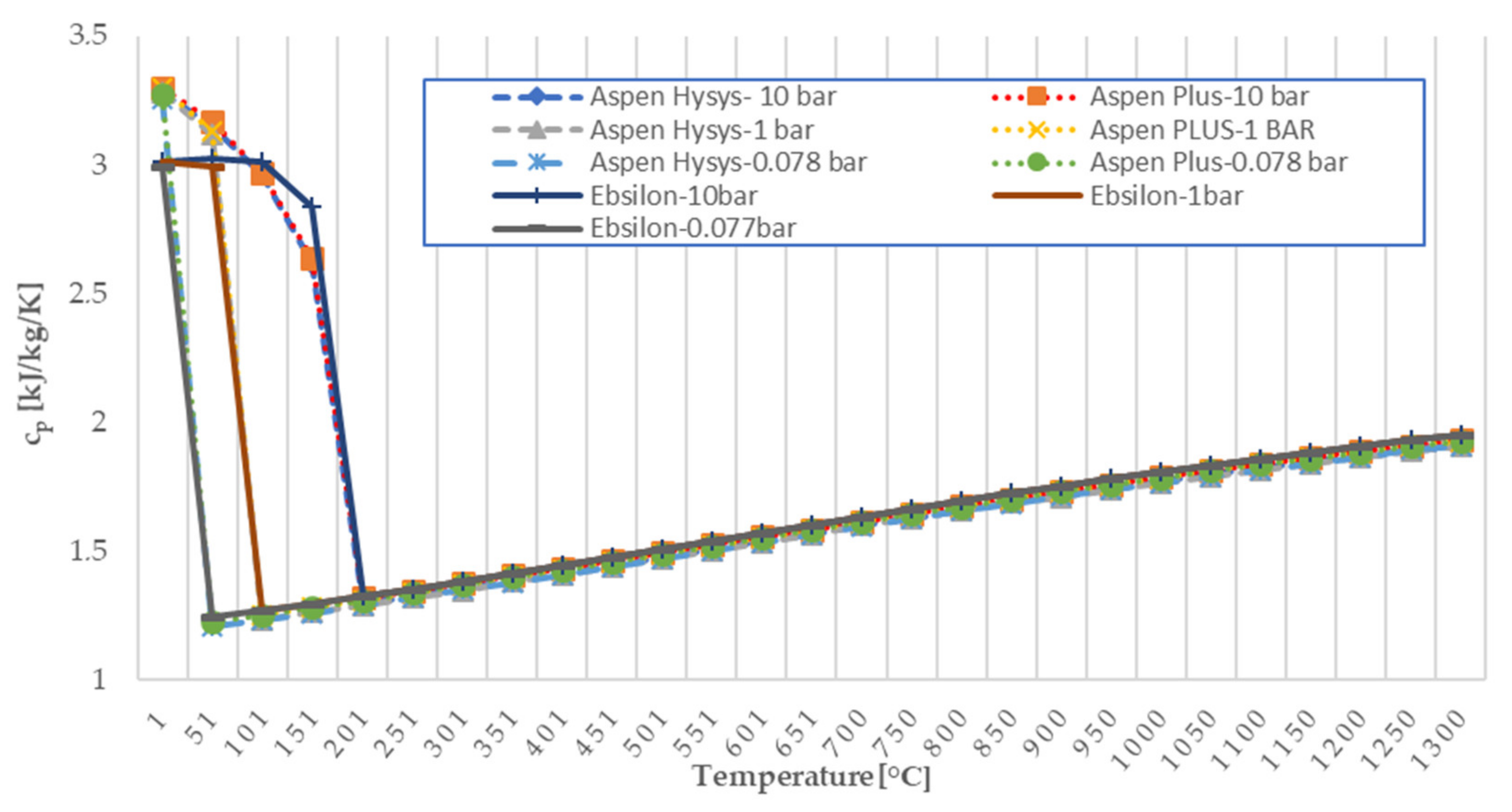
6. Effect of Specific Heat Capacity

The specific heat capacity (also simply specific heat) of a substance is the heat capacity per unit mass of that substance. Here, we shall discuss the specific heat capacity using SI units (kJ/kg∙K). Heat capacity can be expressed at a constant volume (c_v) or constant pressure (c_p). Specific heat capacity of mixture 1 at a constant pressure and volume as a function of temperature from 1 °C to 1300 °C, calculated using Aspen Hysys, Aspen Plus, and Ebsilon, are presented in Figure 13 and Figure 14, respectively.

It can be regarded that c_p and c_v are faced with a decreased trend from 1 °C to 200 °C, so that the minimum value of c_p and c_v is 1.78 kJ/kg∙K and 1.32 kJ/kg∙K at 200 °C, respectively. After that, they increase with rising the temperature. In addition, for T ≥ 200 °C, the specific heat capacity at constant volume (c_v) and constant pressure (c_p) remain approximately constant with increasing the pressure from 0.078 to 10 bar. Specific heat capacity (c_p) in nodal points for at 10 bar and 1100 °C for Aspen Hysys, Aspen Plus, and Ebsilon is represented. It may be viewed that the minimum value (0.92) of c_p belongs to oxygen, whilst the maximum one belongs to water (Figure 15). In addition, there is a direct relation between increasing temperature and c_p. The specific heat capacity values extracted from the codes are close to each other, but when the processes in the individual devices are taken into account, they affect the efficiency values of the whole cycle, in both considered versions of the nCO2PP cycle.

7. Conclusions

The developed version of the cycle, called Process Flow Diagram 0 (“PFD0”), offered the possibility to perform a preliminary assessment of the main cycle parameters, generated power output, as well as temperature in the combustion chamber and at the turbine outlet. It could be concluded that the proposed design of the negative power plant could be considered feasible and competitive with other types BECCS plant, presented in the literature, especially when achievable negative emissions (−720 kg_CO2/MWh_el) are taken into the account.

On the basis of the obtained results, the following key conclusions can be presented:

(1)

The presented cycle “PFD0” allows generating approx. 150 kW for mixture 1 and 160 kW for methane in three considered software (Table 9).

(2)

When inflicting the same mass flow rates (oxygen, water, mixture 1, or methane) and temperatures as in Ebsilon at the inlet to the combustion chamber, we obtain a temperature higher by 27 or 9 degrees Celsius or more in Aspen Plus and Aspen Hysys, and therefore the temperature at the exit from the WCC is 1073 or 1091 °C.

(3)

On the other hand, when given the same mass flow rates (oxygen, water, mixture 1 or methane) and different temperatures downstream of the heat exchanger in the Ebsilon, the temperature downstream of the combustion chamber can be constant, so the WCC plot is 1100 °C.

(4)

The trend is similar for mixture 1 and methane, but the differences are greater as we do not have the same set of reactions concerning the combustion chamber. In this case, the conversion of the ammonia combustion reaction to NO and H₂O to combustion to N₂ and H₂O gives a gain of 6 degrees Celsius more (see Table 11). In mixture 1, we have significant ammonia content why explains the large difference with respect to combustion in traditional chambers, where this influence is negligible.

(5)

An argument that a likely reason for the differences in the two codes are the different definitions, e.g., in one specific heat capacity of steam stabilized in Ebsilon and in Aspen specific heat capacity of steam following the P-R equation, is the fact that we obtain different temperatures after the pump and after the compressors with assumed isentropic efficiencies at the same level, at the same inlet temperatures, and at the same pressure rise (see Section 6).

Additionally, the proposed version of the cycle, called the process flow diagram 1 (“PFD1”), offered the possibility to perform a preliminary assessment of the main cycle parameters, consumed and generated powers, efficiencies, and temperatures in nodal points. The following conclusions can be drawn from Section 4 and Section 5:

(1)

SEC significantly affects the efficiency of the cycle but provides the opportunity for carbon dioxide separation in the nCO2PP system.

(2)

Differences in the Aspen Plus, Aspen Hysys, and Ebsilon codes follow a similar trend.

(3)

In subsequent calculations, the modeling of the injector should be approached more extensively. For example, there should be more reliance on measurement results obtained from one’s own experiment.

(4)

The possibility of a negative CO₂ emission power plant and the positive environmental impact of the proposed solution were demonstrated.

References

1. United Nations Framework Convention on Climate Change—Paris Agreement. Available online: https://unfccc.int/process-and-meetings/the-paris-agreement/the-paris-agreement (accessed on 1 July 2021).
2. Masson-Delmotte, V.; Zhai, P.; Pörtner, H.-O.; Roberts, D.; Skea, J.; Shukla, P.R.; Pirani, A.; Moufouma-Okia, W.; Péan, C.; Pidcock, R.; et al. Global Warming of 1.5 °C; IPCC—The Intergovernmental Panel on Climate Change: Geneva, Switzerland, 2019. [Google Scholar]
3. Friedlingstein, P.; Jones, M.W.; O’Sullivan, M.; Andrew, R.M.; Hauck, J.; Peters, G.P.; Peters, W.; Pongratz, J.; Sitch, S.; Le Quéré, C.; et al. Global Carbon Budget 2019. Earth Syst. Sci. Data 2019, 11, 1783–1838. [Google Scholar] [CrossRef] [Green Version]
4. Romanak, K.; Fridahl, M.; Dixon, T. Attitudes on Carbon Capture and Storage (CCS) as a Mitigation Technology within the UNFCCC. Energies 2021, 14, 629. [Google Scholar] [CrossRef]
5. Hiremath, M.; Viebahn, P.; Samadi, S. An Integrated Comparative Assessment of Coal-Based Carbon Capture and Storage (CCS) Vis-à-Vis Renewable Energies in India’s Low Carbon Electricity Transition Scenarios. Energies 2021, 14, 262. [Google Scholar] [CrossRef]
6. Sifat, N.S.; Haseli, Y. A Critical Review of CO2 Capture Technologies and Prospects for Clean Power Generation. Energies 2019, 12, 4143. [Google Scholar] [CrossRef] [Green Version]
7. Qvist, S.; Gładysz, P.; Bartela, L.; Sowiżdżał, A. Retrofit Decarbonization of Coal Power Plants—A Case Study for Poland. Energies 2020, 14, 120. [Google Scholar] [CrossRef]
8. Gładysz, P.; Sowiżdżał, A.; Miecznik, M.; Hacaga, M.; Pająk, L. Techno-Economic Assessment of a Combined Heat and Power Plant Integrated with Carbon Dioxide Removal Technology: A Case Study for Central Poland. Energies 2020, 13, 2841. [Google Scholar] [CrossRef]
9. Gładysz, P.; Stanek, W.; Czarnowska, L.; Węcel, G.; Langørgen, Ø. Thermodynamic assessment of an integrated MILD oxyfuel combustion power plant. Energy 2017, 137, 761–774. [Google Scholar] [CrossRef]
10. Gładysz, P.; Stanek, W.; Czarnowska, L.; Sładek, S.; Szlęk, A. Thermo-ecological evaluation of an integrated MILD oxy-fuel combustion power plant with CO2 capture, utilisation, and storage—A case study in Poland. Energy 2018, 144, 379–392. [Google Scholar] [CrossRef]
11. Míguez, J.L.; Porteiro, J.; Pérez-Orozco, R.; Gómez, M. Technology Evolution in Membrane-Based CCS. Energies 2018, 11, 3153. [Google Scholar] [CrossRef] [Green Version]
12. Sieradzka, M.; Gao, N.; Quan, C.; Mlonka-Mędrala, A.; Magdziarz, A. Biomass Thermochemical Conversion via Pyrolysis with Integrated CO2 Capture. Energies 2020, 13, 1050. [Google Scholar] [CrossRef] [Green Version]
13. Cannone, S.F.; Lanzini, A.; Santarelli, M. A Review on CO2 Capture Technologies with Focus on CO2-Enhanced Methane Recovery from Hydrates. Energies 2021, 14, 387. [Google Scholar] [CrossRef]
14. Arora, A.; Kumar, A.; Bhattacharjee, G.; Kumar, P.; Balomajumder, C. Effect of different fixed bed media on the performance of sodium dodecyl sulfate for hydrate based CO2 capture. Mater. Des. 2016, 90, 1186–1191. [Google Scholar] [CrossRef]
15. Arora, A.; Kumar, A.; Bhattacharjee, G.; Balomajumder, C.; Kumar, P. Hydrate-Based Carbon Capture Process: Assessment of Various Packed Bed Systems for Boosted Kinetics of Hydrate Formation. J. Energy Resour. Technol. 2020, 143, 033005. [Google Scholar] [CrossRef]
16. Detz, R.J.; van der Zwaan, B. Transitioning towards negative CO2 emissions. Energy Policy 2019, 133, 110938. [Google Scholar] [CrossRef]
17. Lisbona, P.; Pascual, S.; Pérez, V. Evaluation of Synergies of a Biomass Power Plant and a Biogas Station with a Carbon Capture System. Energies 2021, 14, 908. [Google Scholar] [CrossRef]
18. Mendiara, T.; García-Labiano, F.; Abad, A.; Gayán, P.; de Diego, L.F.; Izquierdo, M.; Adánez, J. Negative CO2 emissions through the use of biofuels in chemical looping technology: A review. Appl. Energy 2018, 232, 657–684. [Google Scholar] [CrossRef]
19. Bhui, B.; Vairakannu, P. Prospects and issues of integration of co-combustion of solid fuels (coal and biomass) in chemical looping technology. J. Environ. Manag. 2018, 231, 1241–1256. [Google Scholar] [CrossRef]
20. Lyngfelt, A.; Johansson, D.J.; Lindeberg, E. Negative CO2 emissions—An analysis of the retention times required with respect to possible carbon leakage. Int. J. Greenh. Gas Control 2019, 87, 27–33. [Google Scholar] [CrossRef]
21. Niu, X.; Shen, L.; Jiang, S.; Gu, H.; Xiao, J. Combustion performance of sewage sludge in chemical looping combustion with bimetallic Cu–Fe oxygen carrier. Chem. Eng. J. 2016, 294, 185–192. [Google Scholar] [CrossRef]
22. Saari, J.; Peltola, P.; Tynjälä, T.; Hyppänen, T.; Kaikko, J.; Vakkilainen, E. High-Efficiency Bioenergy Carbon Capture Integrating Chemical Looping Combustion with Oxygen Uncoupling and a Large Cogeneration Plant. Energies 2020, 13, 3075. [Google Scholar] [CrossRef]
23. Buscheck, T.A.; Upadhye, R.S. Hybrid-energy approach enabled by heat storage and oxy-combustion to generate electricity with near-zero or negative CO2 emissions. Energy Convers. Manag. 2021, 244, 114496. [Google Scholar] [CrossRef]
24. Pawlak-Kruczek, H.; Niedzwiecki, L.; Ostrycharczyk, M.; Czerep, M.; Plutecki, Z. Potential and methods for increasing the flexibility and efficiency of the lignite fired power unit, using integrated lignite drying. Energy 2019, 181, 1142–1151. [Google Scholar] [CrossRef]
25. Madejski, P.; Żymełka, P. Calculation methods of steam boiler operation factors under varying operating conditions with the use of computational thermodynamic modeling. Energy 2020, 197, 117221. [Google Scholar] [CrossRef]
26. Modliński, N.; Szczepanek, K.; Nabagło, D.; Madejski, P.; Modliński, Z. Mathematical procedure for predicting tube metal temperature in the second stage reheater of the operating flexibly steam boiler. Appl. Therm. Eng. 2019, 146, 854–865. [Google Scholar] [CrossRef]
27. Mączka, T.; Pawlak-Kruczek, H.; Niedzwiecki, L.; Ziaja, E.; Chorążyczewski, A. Plasma Assisted Combustion as a Cost-Effective Way for Balancing of Intermittent Sources: Techno-Economic Assessment for 200 MWel Power Unit. Energies 2020, 13, 5056. [Google Scholar] [CrossRef]
28. Benato, A.; Bracco, S.; Stoppato, A.; Mirandola, A. LTE: A procedure to predict power plants dynamic behaviour and components lifetime reduction during transient operation. Appl. Energy 2016, 162, 880–891. [Google Scholar] [CrossRef]
29. Capron, M.; Stewart, J.; N’Yeurt, A.D.R.; Chambers, M.; Kim, J.; Yarish, C.; Jones, A.; Blaylock, R.; James, S.; Fuhrman, R.; et al. Restoring Pre-Industrial CO2 Levels While Achieving Sustainable Development Goals. Energies 2020, 13, 4972. [Google Scholar] [CrossRef]
30. Cheng, F.; Small, A.A.; Colosi, L.M. The levelized cost of negative CO2 emissions from thermochemical conversion of biomass coupled with carbon capture and storage. Energy Convers. Manag. 2021, 237, 114115. [Google Scholar] [CrossRef]
31. EU Carbon Price Hits Record 50 Euros per Tonne on Route to Climate Target|Reuters. Available online: https://www.reuters.com/business/energy/eu-carbon-price-tops-50-euros-first-time-2021-05-04/ (accessed on 7 August 2021).
32. Restrepo-Valencia, S.; Walter, A. Techno-Economic Assessment of Bio-Energy with Carbon Capture and Storage Systems in a Typical Sugarcane Mill in Brazil. Energies 2019, 12, 1129. [Google Scholar] [CrossRef] [Green Version]
33. Mikielewicz, D.; Wajs, J.; Ziółkowski, P.; Mikielewicz, J. Utilisation of waste heat from the power plant by use of the ORC aided with bleed steam and extra source of heat. Energy 2016, 97, 11–19. [Google Scholar] [CrossRef]
34. Szablowski, L.; Krawczyk, P.; Badyda, K.; Karellas, S.; Kakaras, E.; Bujalski, W. Energy and exergy analysis of adiabatic compressed air energy storage system. Energy 2017, 138, 12–18. [Google Scholar] [CrossRef]
35. Bartela, L.; Skorek-Osikowska, A.; Kotowicz, J. Economic analysis of a supercritical coal-fired CHP plant integrated with an absorption carbon capture installation. Energy 2014, 64, 513–523. [Google Scholar] [CrossRef]
36. Zymelka, P.; Szega, M.; Madejski, P. Techno-Economic Optimization of Electricity and Heat Production in a Gas-Fired Combined Heat and Power Plant with a Heat Accumulator. J. Energy Resour. Technol. 2020, 142, 022101. [Google Scholar] [CrossRef]
37. Kotowicz, J.; Job, M.; Brzęczek, M. The characteristics of ultramodern combined cycle power plants. Energy 2015, 92, 197–211. [Google Scholar] [CrossRef]
38. Topolski, J.; Badur, J. Efficiency of HRSG within a Combined Cycle with gasification and sequential combustion at GT26 Turbine. In Proceedings of the Second International Scientific Symposium Compower, Gdańsk, Poland, 4–7 September 2000; pp. 291–298. [Google Scholar]
39. Ziółkowski, P.; Badur, J.; Ziółkowski, P. An energetic analysis of a gas turbine with regenerative heating using turbine extraction at intermediate pressure - Brayton cycle advanced according to Szewalski’s idea. Energy 2019, 185, 763–786. [Google Scholar] [CrossRef]
40. Głuch, J. Selected problems of determining an efficient operation standard in contemporary heat-and-flow diagnostics. Pol. Marit. Res. 2009, 16, 22–26. [Google Scholar] [CrossRef]
41. Ong’Iro, A.; Ugursal, V.; Al Taweel, A.; Lajeunesse, G. Thermodynamic simulation and evaluation of a steam CHP plant using ASPEN Plus. Appl. Therm. Eng. 1996, 16, 263–271. [Google Scholar] [CrossRef]
42. Liu, B.; Yang, X.-M.; Song, W.-L.; Lin, W.-G. Process simulation of formation and emission of NO and N2O during coal decoupling combustion in a circulating fluidized bed combustor using Aspen Plus. Chem. Eng. Sci. 2012, 71, 375–391. [Google Scholar] [CrossRef]
43. Jang, D.-H.; Kim, H.-T.; Lee, C.; Kim, S.-H. Kinetic analysis of catalytic coal gasification process in fixed bed condition using Aspen Plus. Int. J. Hydrogen Energy 2013, 38, 6021–6026. [Google Scholar] [CrossRef]
44. Nikoo, M.B.; Mahinpey, N. Simulation of biomass gasification in fluidized bed reactor using ASPEN PLUS. Biomass Bioenergy 2008, 32, 1245–1254. [Google Scholar] [CrossRef]
45. Damartzis, T.; Michailos, S.; Zabaniotou, A. Energetic assessment of a combined heat and power integrated biomass gasification–internal combustion engine system by using Aspen Plus®. Fuel Process. Technol. 2012, 95, 37–44. [Google Scholar] [CrossRef]
46. Steag Energy Services Ebsilon®Professional 15.00. Available online: https://www.ebsilon.com/ (accessed on 22 September 2021).
47. Madejski, P.; Żymełka, P. Introduction to Computer Calculations and Simulation of Energy Systems Operation in STEAG Eb-silon®Professional; Wydawnictwa AGH: Kraków, Poland, 2020. [Google Scholar]
48. Soares, J.; Oliveira, A.; Valenzuela, L. A dynamic model for once-through direct steam generation in linear focus solar collectors. Renew. Energy 2021, 163, 246–261. [Google Scholar] [CrossRef]
49. Yue, M.; Ma, G.; Shi, Y. Analysis of Gas Recirculation Influencing Factors of a Double Reheat 1000 MW Unit with the Reheat Steam Temperature under Control. Energies 2020, 13, 4253. [Google Scholar] [CrossRef]
50. Dahash, A.; Mieck, S.; Ochs, F.; Krautz, H.J. A comparative study of two simulation tools for the technical feasibility in terms of modeling district heating systems: An optimization case study. Simul. Model. Pract. Theory 2018, 91, 48–68. [Google Scholar] [CrossRef]
51. Mondal, S.K.; Uddin, M.F.; Majumder, S.; Pokhrel, J. HYSYS Simulation of Chemical Process Equipments. Available online: https://www.researchgate.net/publication/281608946_HYSYS_Simulation_of_Chemical_Process_Equipments (accessed on 22 September 2021).
52. Ziółkowski, P.; Kowalczyk, T.; Kornet, S.; Badur, J. On low-grade waste heat utilization from a supercritical steam power plant using an ORC-bottoming cycle coupled with two sources of heat. Energy Convers. Manag. 2017, 146, 158–173. [Google Scholar] [CrossRef]
53. Ziółkowski, P.; Kowalczyk, T.; Lemański, M.; Badur, J. On energy, exergy, and environmental aspects of a combined gas-steam cycle for heat and power generation undergoing a process of retrofitting by steam injection. Energy Convers. Manag. 2019, 192, 374–384. [Google Scholar] [CrossRef]
54. Werle, S.; Wilk, R.K. A review of methods for the thermal utilization of sewage sludge: The Polish perspective. Renew. Energy 2010, 35, 1914–1919. [Google Scholar] [CrossRef]
55. Schweitzer, D.; Gredinger, A.; Schmid, M.; Waizmann, G.; Beirow, M.; Spörl, R.; Scheffknecht, G. Steam gasification of wood pellets, sewage sludge and manure: Gasification performance and concentration of impurities. Biomass Bioenergy 2018, 111, 308–319. [Google Scholar] [CrossRef]
56. Akkache, S.; Hernández, A.-B.; Teixeira, G.; Gelix, F.; Roche, N.; Ferrasse, J.H. Co-gasification of wastewater sludge and different feedstock: Feasibility study. Biomass Bioenergy 2016, 89, 201–209. [Google Scholar] [CrossRef] [Green Version]
57. Bonalumi, D.; Valenti, G.; Lillia, S.; Fosbol, P.L.; Thomsen, K. A layout for the Carbon Capture with Aqueous Ammonia without Salt Precipitation. Energy Procedia 2016, 86, 134–143. [Google Scholar] [CrossRef] [Green Version]
58. Campanari, S.; Chiesa, P.; Manzolini, G. CO2 capture from combined cycles integrated with Molten Carbonate Fuel Cells. Int. J. Greenh. Gas Control 2010, 4, 441–451. [Google Scholar] [CrossRef]
59. Gou, C.; Cai, R.; Hong, H. An Advanced Oxy-Fuel Power Cycle with High Efficiency. Proc. Inst. Mech. Eng. Part A J. Power Energy 2006, 220, 315–325. [Google Scholar] [CrossRef]
60. Liu, C.; Chen, G.; Sipöcz, N.; Assadi, M.; Bai, X. Characteristics of oxy-fuel combustion in gas turbines. Appl. Energy 2012, 89, 387–394. [Google Scholar] [CrossRef]
Figure 1. Process flow diagram of a gas mixture cycle PFD0—a steam-gas turbine system (0FUEL, 0O2, 01-H2O, 02-H2O, 1FUEL, 1O2, 1H2O, 2, 3, 4, 5—cycle nodal points).
Energies 14 06304 g001
Figure 2. Simulation of PFD0 by Aspen Hysys (0FUEL, 0O2, 01-H2O, 02-H2O, 1FUEL, 1O2, 1H2O, 2, 3, 4, 5—cycle nodal points).
Energies 14 06304 g002
Figure 3. Simulation of PFD0 by Aspen Plus (0FUEL, 0O2, 01-H2O, 02-H2O, 1FUEL, 1O2, 1H2O, 2, 3, 4, 5—cycle nodal points).
Energies 14 06304 g003
Figure 4. Simulation of PFD0 by Ebsilon (0FUEL, 0O2, 01-H2O, 02-H2O, 1FUEL, 1O2, 1H2O, 2, 3, 4, 5—cycle nodal points).
Energies 14 06304 g004
Figure 5. Fuel compositions for the analysed cycle.
Energies 14 06304 g005
Figure 6. Process flow diagram of a gas mixture cycle—a steam-gas turbine system, where: WCC—wet combustion chamber; SEC—spray ejector condenser; R—gasifier (Reactor); GT—gas–steam turbine; GTbap—gas–steam turbine—below ambient pressure; Cfuel—fuel compressor; CO2—oxygen compressor; CCO2-1,2—CO2 capture unit compressors 1 and 2; PH2O—water pump supplying supercritical water; PSEC—water pump supplying SEC, S + HE2—separator with heat exchanger 2; HE 1, 3, and 4—heat exchanger 1, 3, and 4; ASU—air separation unit; GS—gas scrubber; G~—power generators; M—motor; LTS—low-temperature source, STCO2—CO2 storage tank. Nodal points—general thermodynamic cycle: 0 FUEL, 0 O2, 1 FUEL, 1 O2, 2, 3, 3’, 4, 5, 6, 7; optional: 2’; CO2 capture unit: 1 CCU, 2 CCU, 3 CCU, 4 CCU, 5 CCU; optional: 2 CCU’, 2 CCU”; SEC: 0 SEC, 1 SEC, 2 SEC; gasifying agent supply: 0 R; optional: 0 R’,1 R; water production: 0 PROD, 1 PROD’, 2 PROD; optional CO2 injection to WCC: 1 CO2; water supply: 0 1-H2O, 0 2-H2O, 0 2-H2O’, 0 2-H2O”,1 H2O, 2 H2O, 3 H2O; optional: 1 H2O’, 1 H2O”, 3 H2O’, 3 H2O”.
Energies 14 06304 g006
Figure 7. Simulation of PFD1 by Aspen HYSYS.
Energies 14 06304 g007
Figure 8. Simulation of PFD1 by Aspen Plus.
Energies 14 06304 g008
Figure 9. Simulation of PFD1 by by Ebsilon.
Energies 14 06304 g009
Figure 10. Exhaust CO2, H2O fraction and mass flow of water production in the cycle for various computing codes (AP—Aspen Plus, AH—Aspen Hysys, Ebs—Ebsilon).
Energies 14 06304 g010
Figure 11. Combined turbine power, chemical energy of mixture 1 and methane combustion, and gross efficiency for various computing codes (AP—Aspen Plus, AH—Aspen Hysys, Ebs—Ebsilon).
Energies 14 06304 g011
Figure 12. Spray ejector condenser 1SEC: Nozzle inlet, a: Nozzle outlet, a–c: Mixing chamber, b: Suction chamber, c: Throat (part of Diffuser), c-2SEC: Diffuser, 5 Inlet of entrained fluid, 5-MC: Entrained fluid in mixing chamber.
Energies 14 06304 g012
Figure 13. Distribution of heat capacity at constant pressure per temperature after WCC at different pressure in Aspen Hysys, Aspen Plus, and Ebsilon.
Energies 14 06304 g013
Figure 14. Distribution of heat capacity at constant volume per temperature after WCC at different pressure in Aspen Hysys, Aspen Plus and Ebsilon.
Energies 14 06304 g014
Figure 15. Specific heat capacity (cp) in nodal points PFD0, mixture 1, WCC exhaust at 10 bar and 1100 °C for Aspen Hysys, Aspen Plus and Ebsilon.
Energies 14 06304 g015