Optimization of a Mixed Refrigerant Based H₂ Liquefaction Pre-Cooling Process and Estimate of Liquefaction Performance with Varying Ambient Temperature

Abstract

Hydrogen used as an energy carrier can provide an important route to the decarbonization of energy supplies, but realizing this opportunity will require both significantly increased production and transportation capacity. One route to increased transportation capacity is the shipping of liquid hydrogen, but this requires an energy-intensive liquefaction step. Recent study work has shown that the energy required in this process can be reduced through the implementation of new and improved process designs, but since all low-temperature processes are affected by the available heat-sink temperature, local ambient conditions will also have an impact. The objective of this work is to identify how the energy consumption associated with hydrogen liquefaction varies with heat-sink temperature through the optimization of design parameters for a next-generation mixed refrigerant based hydrogen liquefaction process. The results show that energy consumption increases by around 20% across the cooling temperature range 5 to 50 °C. Considering just the range 20 to 30 °C, there is a 5% increase, illustrating the significant impact ambient temperature can have on energy consumption. The implications of this work are that the modelling of different liquified hydrogen based energy supply chains should take the impact of ambient temperature into account.

1. Introduction

Hydrogen used as a fuel, as an energy source for industrial processes or for generating electrical power can provide an important route to the decarbonization of energy supplies and the integration of renewable energy systems. The study of Acar and Dincer [1], for example, identifies that hydrogen can play “eight significant roles” in the green energy transition. Recent studies have also made the case that achieving a transition to carbon-free energy in the EU is impossible without a large increase in hydrogen production [2], and energy system modeling has found that “hydrogen and synfuels add up to between 20% and 50% of [EU] energy demand in transport in 2050” [3]. This positive view of the role that hydrogen could play in future low-carbon development is also reflected in political intent via the EU hydrogen strategy [4].

Reflecting this political support, research related to hydrogen energy has increased over recent years [5]. Important research topics include energy demand and supply modelling [2,3], the novel integration of renewable energy sources such as solar power [6], the development of enhanced electrolysis based production methods [7], the development of new applications such as use a reductant in steel manufacturing [8] and the assessment of alternative sources such as methanol [9].

In all envisaged future hydrogen-based economies, a significant increase in the transportation capacity for hydrogen is required. It is possible to transport hydrogen as a compressed gas or as a liquid at low temperature, in pipelines as a gas. The optimum transportation strategy will depending on both transportation capacity and the distance [10]. When the distance is significant it is reasonable to expect that shipping of hydrogen will be favored, and while researchers such as Ishimoto et al. [11] have studied the economics of shipping liquefied hydrogen, some commercial steps have also been made, with the world’s first liquid hydrogen carrier ship launched in Japan in 2019 [12].

If hydrogen is transported at large-scale as a liquid, a key part of the supply chain will be the liquefaction process, which is very energy intensive. The specific energy consumption (SEC) of the most efficient currently operating large-scale hydrogen liquefaction (LHL) plants lies in the range 13 to 15 kWh/kg [13], which is much higher that even the most efficient LNG processes, which have a SEC of around 240 kWh/tonne. Because of this, there is significant interest in the development of new and improved LHL technologies that can help reduced SEC.

Research topics relating to improved LHL technologies include the integration of renewable energy sources, such as solar energy [14] and geothermal energy [15]; the use of mixed refrigerants (MR) for pre-cooling [16,17,18]; and the use of helium in the cryogenic cooling and liquefaction part of the process [19,20]. Other research has focused on the impact of the conversion of ortho-hydrogen to para-hydrogen on the liquefaction process [21,22] and the relative performance of different heat exchanger types [17,22,23]. The suggested efficiency of the proposed concepts for LHL studied lie in the range 5 to 8 kWh/kg [13], which represents a substantial motivation for the implementation of these technologies in the next generation of LHL plants.

The proposed use of a MR in the pre-cooling part of LHL processes represents a close parallel to the use of MR in the design of some of the largest and most efficient natural gas liquefaction processes and because of this, represents one of the most promising near-future improvements to LHL design. LNG plants based on the use of MRs include the Snøhvit plant located at Melkøya in northern Norway, which uses a cascade of three MR loops and is claimed to be the most efficient LNG plant in the world [24]. While the efficiency achieved by the Snøhvit LNG plant is due, in part, to its advanced design, the plant also benefits from its cold-climate location and subsequent access to a lower temperature heat sink than most other LNG plants.

The study of Rian and Ertesvåg [25] looked at the impact of ambient temperature on the Snøhvit LNG plant, finding that a reduction in the available heat sink temperature from 20 to 4 °C gives a reduction in exergy destruction of 10.9%. A small number of other studies have also considered the impact of ambient temperature on the performance of other types of LNG process [26,27,28,29] providing similar results. The study of Park et al., for example, finds that specific power consumption of single MR process increases by between 16% and 42% over the temperature range 10 to 25 °C, varying with the approach used in process optimization. This significance of this variation in energy consumption with ambient temperature is not only relevant to the design of LNG plant itself, it is large enough to affect the whole energy supply chain. For example, the study of Jackson et al. [29] finds that the CO₂ emissions for a power plant supplied by gas from an LNG plant located in northern Norway will be between 0.8 and 1.3% lower than if it were supplied by the same design of LNG plant located in the Middle East. It is therefore logical to expect that the performance of LHL plants using MR pre-cooling and the performance of energy supply chains based on LHL will be significantly affected by the ambient temperature at the liquefaction plant location.

Given the close parallel between MR based LNG processes and MR pre-cooled LHL processes and given the demonstrated impact of ambient temperature the performance of LNG processes, ambient temperature can be expected to have a significant impact on the performance of the type of LHL processes likely to be used in the near future. Although several studies have been made into the performance of MR pre-cooled type LHL process and studies have looked at the impact of ambient temperature on LNG process performance, no studies quantifying this impact of ambient temperature on LHL processes are currently found in the literature. The aim of this study is, therefore, to generate a set of data illustrating the impact of ambient temperature on the performance of MR pre-cooled type LHL process.

2. Materials and Methods

2.1. Selection of the Modeling Basis

Although only a handful different types of liquefaction process are used in current operating LHL plants, a wide range of improved processes have been proposed. In the present study a comprehensive review of the various improved liquefaction technologies is outside the scope of work. Instead, a single, representative, improved process was selected to be used as the basis for the present study. The details of the selection process are described below.

Because the results from this study are intended to support further research in future low-carbon energy supply and, specifically, how different supply chain configurations affect efficiency, the improved concepts of most relevance are those technologies likely to be used in the near future. Taking the techno-economic analysis of Cardella et al. [30] as a basis, the improved technology that fits best with the aim of the study is the use of a mixed refrigerant (MR) for pre-cooling of the hydrogen feed stream.

Most current, and much improved, hydrogen liquefaction processes are based on the division of the overall process into two parts: a pre-cooling step and a cryogenic-cooling step. In conventional LHL plant designs, the pre-cooling stage often uses liquid nitrogen (LIN) as a refrigerant, whereas the cryogenic-cooling step uses either helium in a Brayton cycle, or hydrogen in a Claude cycle [18]. In the cryogenic step, the hydrogen feed is generally cooled from below around −90 °C to the final liquefaction temperature. Although the break-point temperature between the pre-cooling and the cryogenic step, $T_{\mathrm{p}}$, is potentially an optimization variable, the present study assumes that the impact of ambient temperature on operating parameters in the cryogenic step is small and, therefore, that $T_{\mathrm{p}}$ can be fixed.

Typical of the concepts for improved energy consumption using MRs is the process studied in the work of Skaugen et al. [17], which is based on a Claude cycle in cryogenic-cooling step and a MR in the pre-cooling step. In this process the pre-cooling step and the portion of the cryogenic step that operates above $T_{\mathrm{p}}$ are not integrated. This allows the present study to consider the optimization of the pre-cooling process independently from the operation of the cryogenic-cooling process. In addition, because the details of the composition and operating conditions for the proposed MR cycle are clearly set-out in the work of Skaugen et al. [17], the present study uses the work of Skaugen as the basis for model development and validation.

Although the operating parameters in the cryogenic-cooling step are assumed fixed in the present study (i.e., they are not affected by ambient temperature), the energy consumption of the cryogenic-cooling cycle compressor is still affected by the exit temperature that the inter and after-coolers, $T_{\mathrm{c}}$, are designed to operate with, which would normally be set relative to the ambient temperature of the seawater, or air, used as the heat-sink. Because of this, modelling of the performance of the cryogenic cycle compressor as it varies with $T_{\mathrm{c}}$ does form part of the present study.

Another important factor in the design and optimization of hydrogen liquefaction processes is the conversion of ortho to para hydrogen. This process releases a significant quantity of heat, affecting both the process design and the selection of optimum operating parameters. The conversion of the ortho isomer during liquefaction is typically promoted using a catalyst. The effectiveness of the catalyst and the residence time in the heat exchangers affects the approach to the equilibrium concentration and, subsequently, the temperature profile in the heat exchangers. However, across the range of temperatures experienced in the pre-cooling process, the equilibrium concentration of para hydrogen varies by less than 5% [21]. Moreover, as in the study of Skaugen et al. [17]—which is a reference case for this study—catalytic conversion is assumed after the pre-cooling process. This will result in a low approach to the equilibrium conversion in the pre-cooling process and, therefore, in this study the modelling of the conversion of ortho to para hydrogen is set outside the scope of work.

2.2. Process Model Development

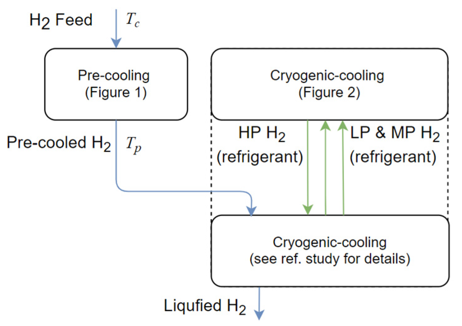
As described above, the process model used in this study consists of two separate parts: a model of the MR pre-cooling step, and a model of the cryogenic-cooling step cycle compressor. The development of these two models is described below. A block diagram showing the relationship between the cryogenic-cooling step and the pre-cooling step is also presented in Appendix A.

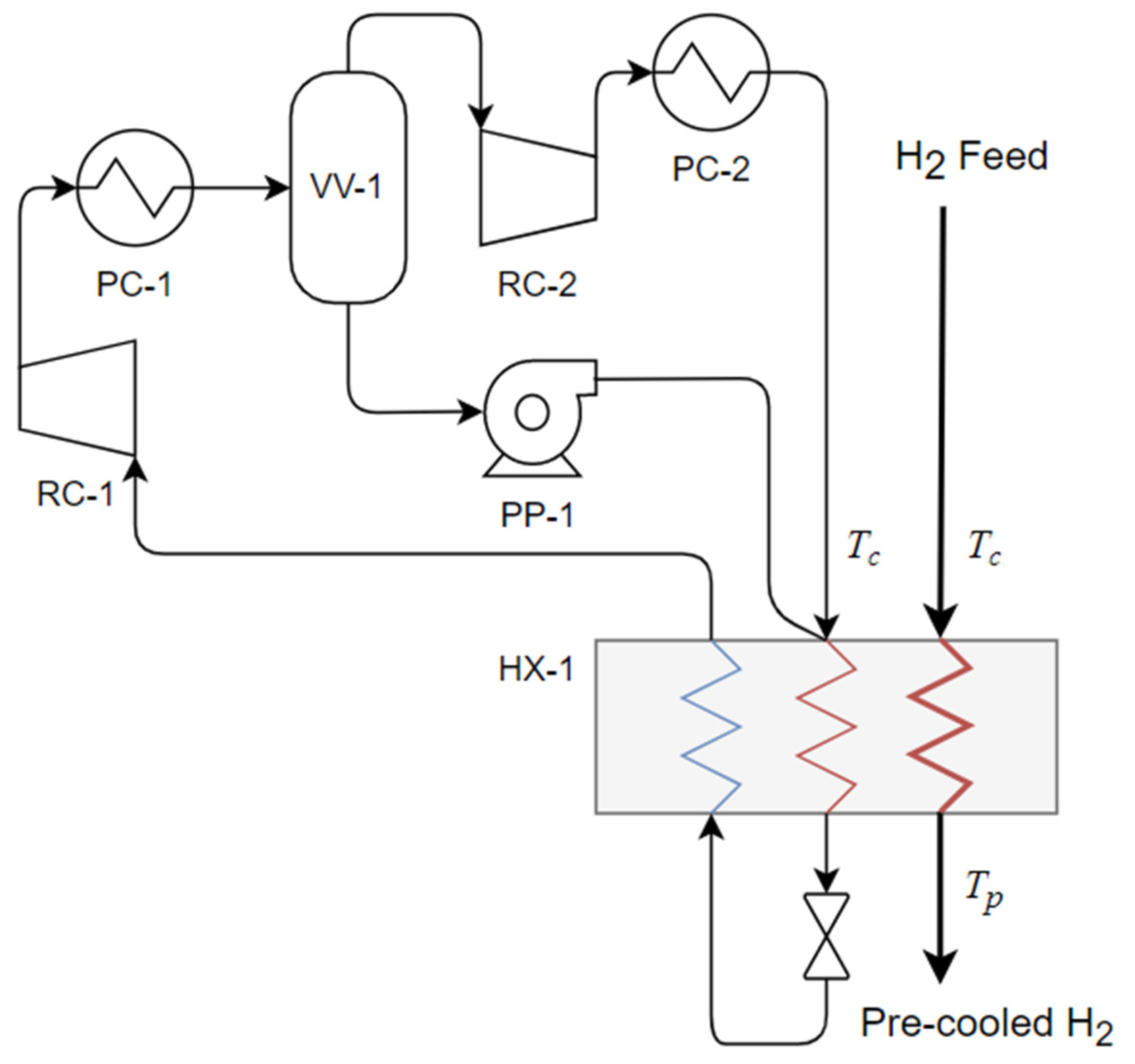
Figure 1 illustrates the process flow scheme used for the MR pre-cooling process, which is based on the flow scheme used in the reference study of Skaugen et al. [17]. The main equipment items shown in Figure 1 are a compressor (comprising RC-1 and RC-2), two process coolers (PC-1 and PC-2), a MR separator (VV-1), a pump (PP-1), and the main heat exchanger (HX-1). The MR compressor comprises two stages (RC-1 and 2), both with after-cooling (PC-1 and 2) to $T_{\mathrm{c}}$. Any liquids condensed liquids after the first stage are separated in VV-1. Liquids separated in this way are pumped (PP-1) to the compressor discharge pressure—bypassing the second stage of compression (RC-2)—and mixed with the vapor stream entering the main heat exchanger (HX-1). The main heat exchanger is modelled as a multi-stream type heat exchanger with two hot streams: H₂ and high-pressure MR, and one cold stream: low-pressure MR. The low-pressure MR stream exiting the main heat exchanger returns to the MR compressor. Hydrogen leaving HX-1 is cooled to $T_{\mathrm{p}}$.

To allow the calculation of process energy consumption a simplified model of the process presented in Figure 1 was developed in MATLAB [31] with the TREND software package [32] used to calculate thermo-physical properties.

Table 1. Summary of MR process fixed modelling parameters.

Parameter	Value	Units
Hydrogen Feed Pressure	20	bara
H2 pre-cooling temperature, $T_p$	−159	°C
Compressor/ pump efficiency	85	% *
HX-1 pressure-loss (hot streams)	0.5	bar
HX-1 pressure-loss (cold streams)	0.1	bar
PC-1 and 2 pressure-loss	0.5	bar

* Isentropic efficiency.

presents the set of fixed modelling parameters, $\mathrm{MP}$, used in the model of the MR pre-cooling process. In general, the parameters in Table 1 were selected to reflect those used in the reference study [17].

For simplicity, the pressure-loss in the main heat exchanger was scaled linearly with temperature and the two MR streams were assumed to be mixed before entering the heat exchanger and the combined MR stream enters the main heat exchanger at the H₂ feed temperature.

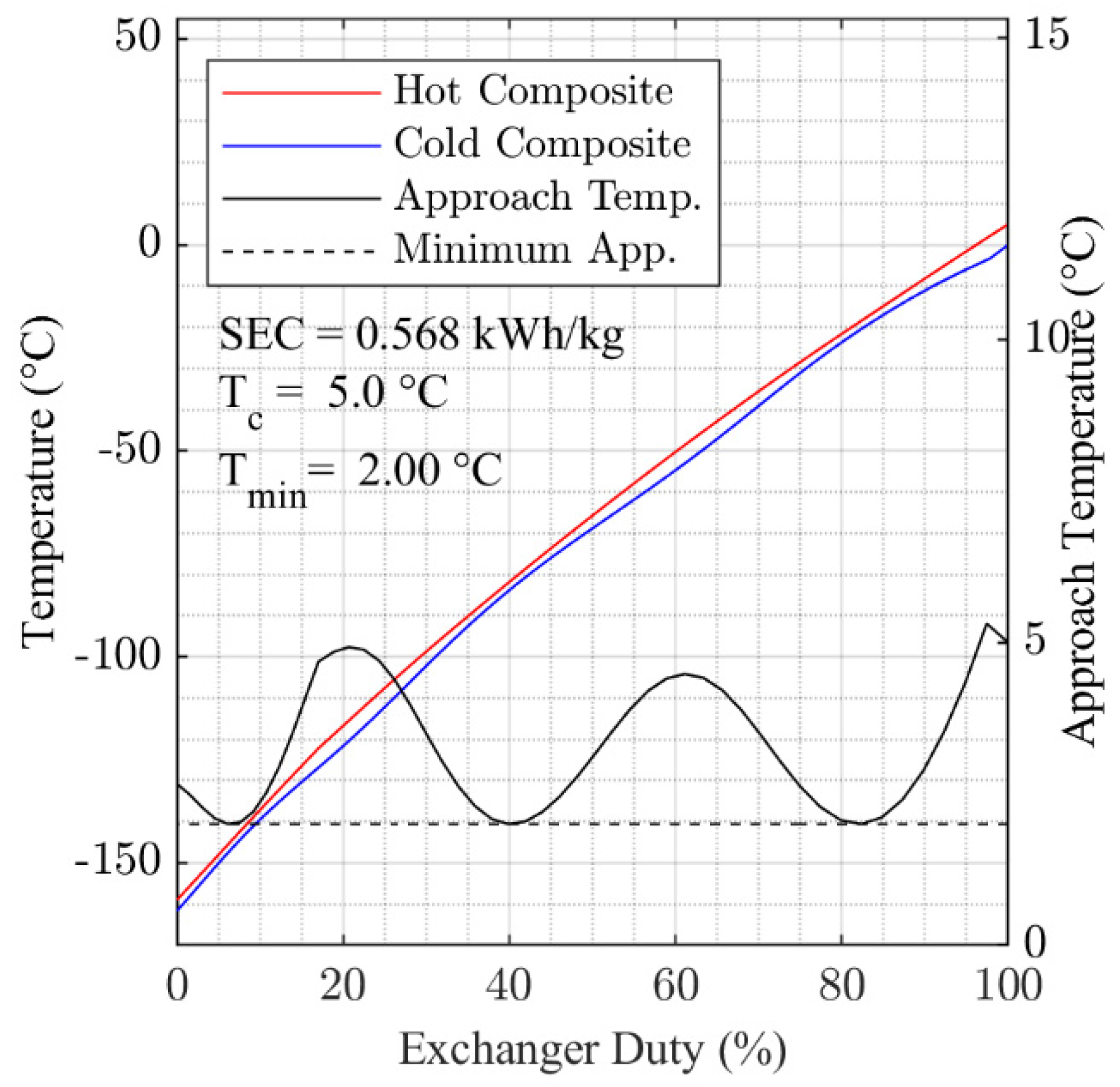
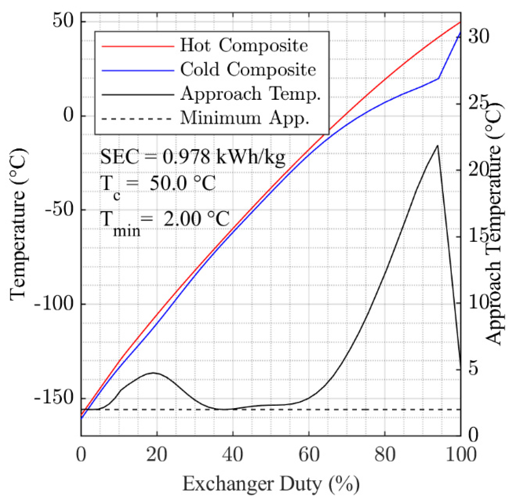
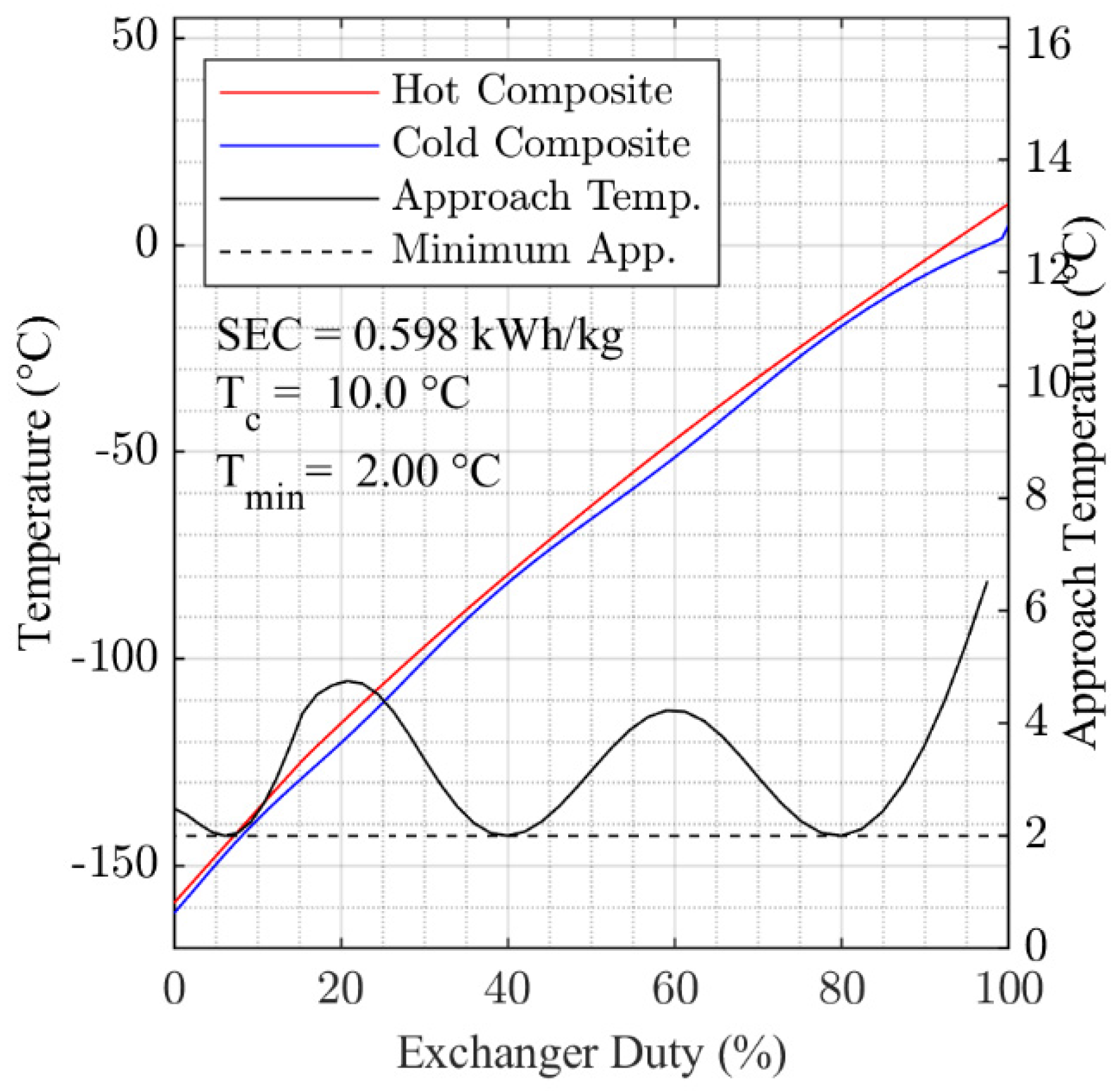
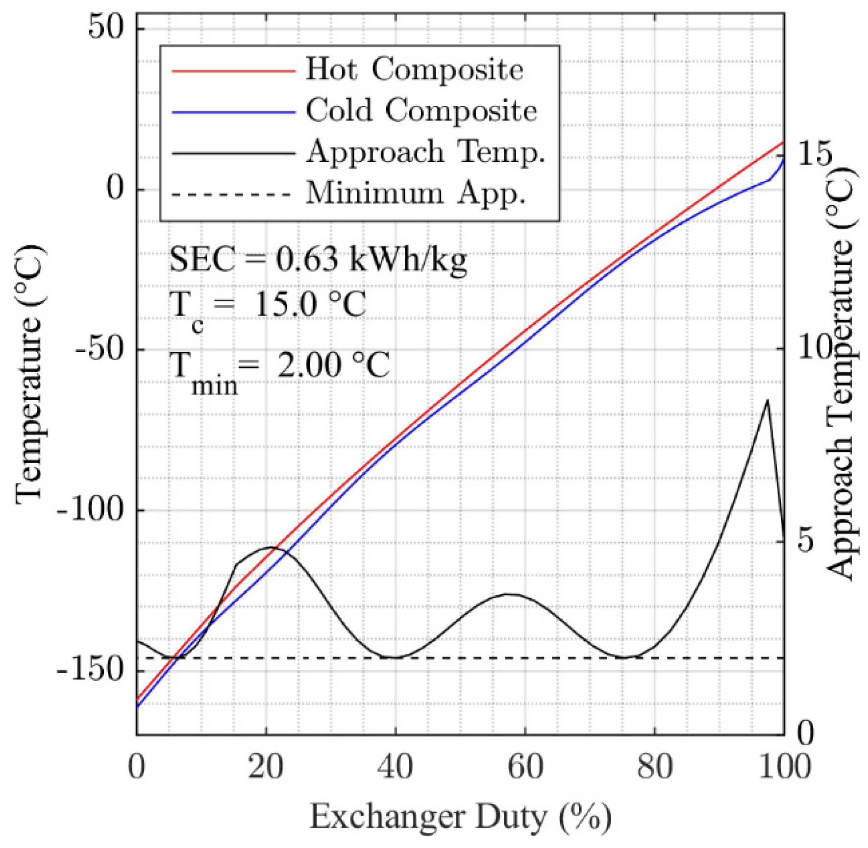
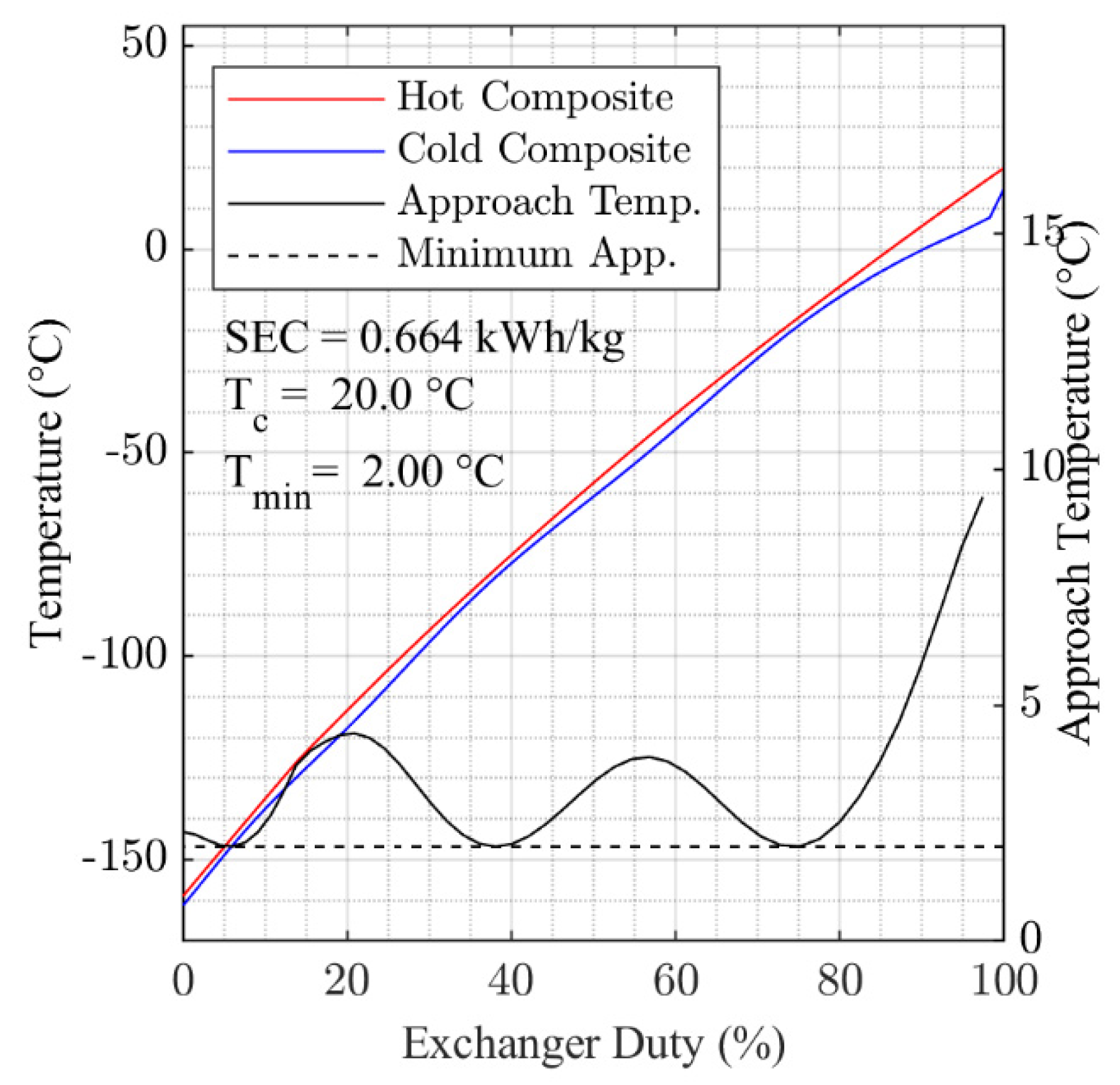
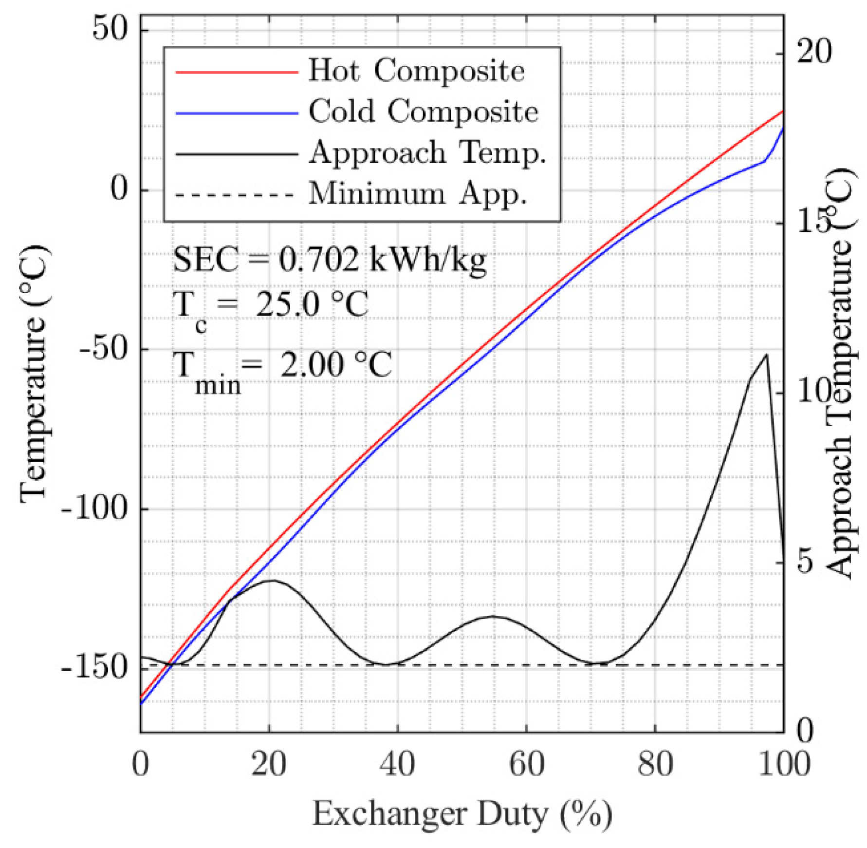
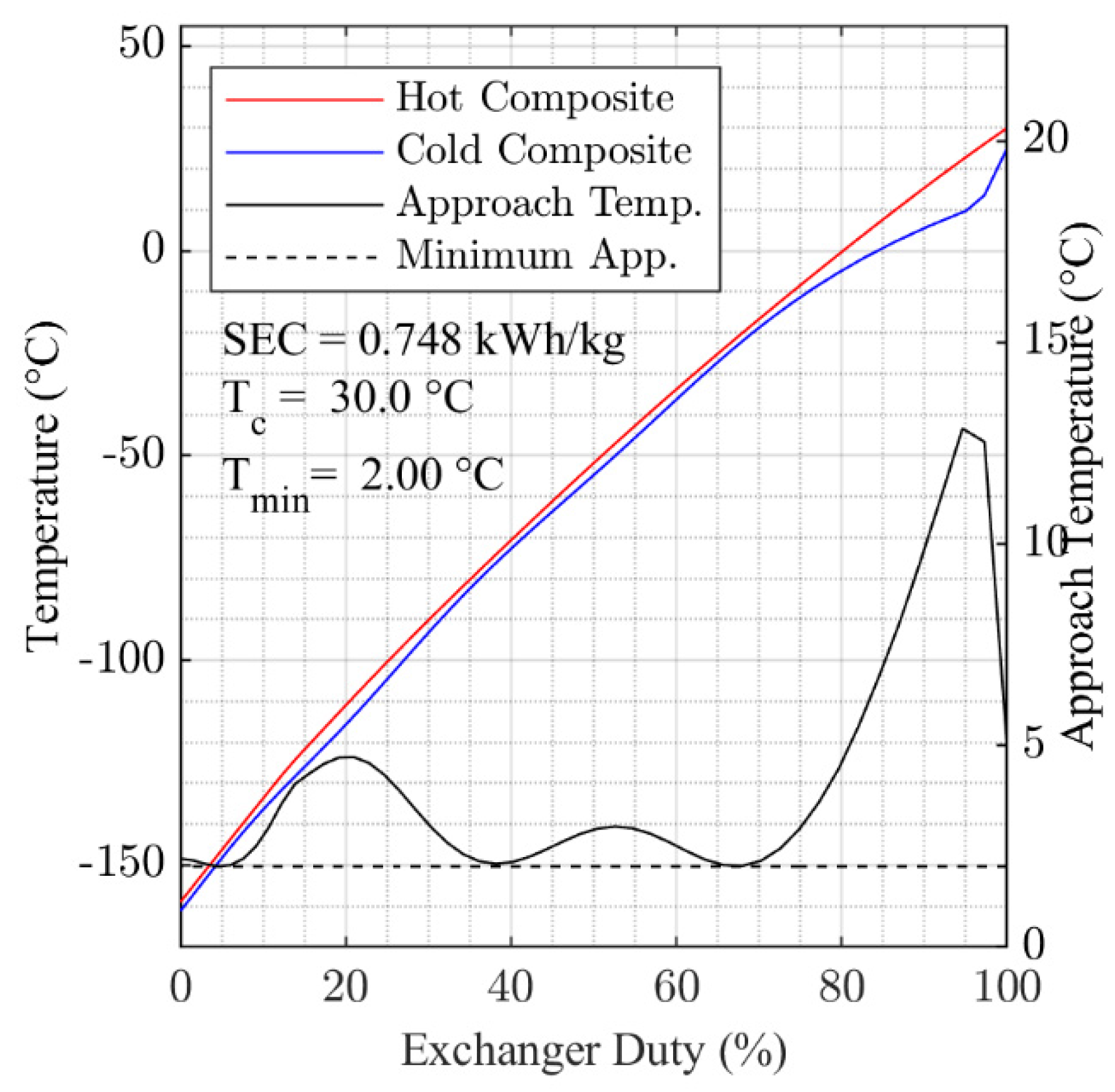
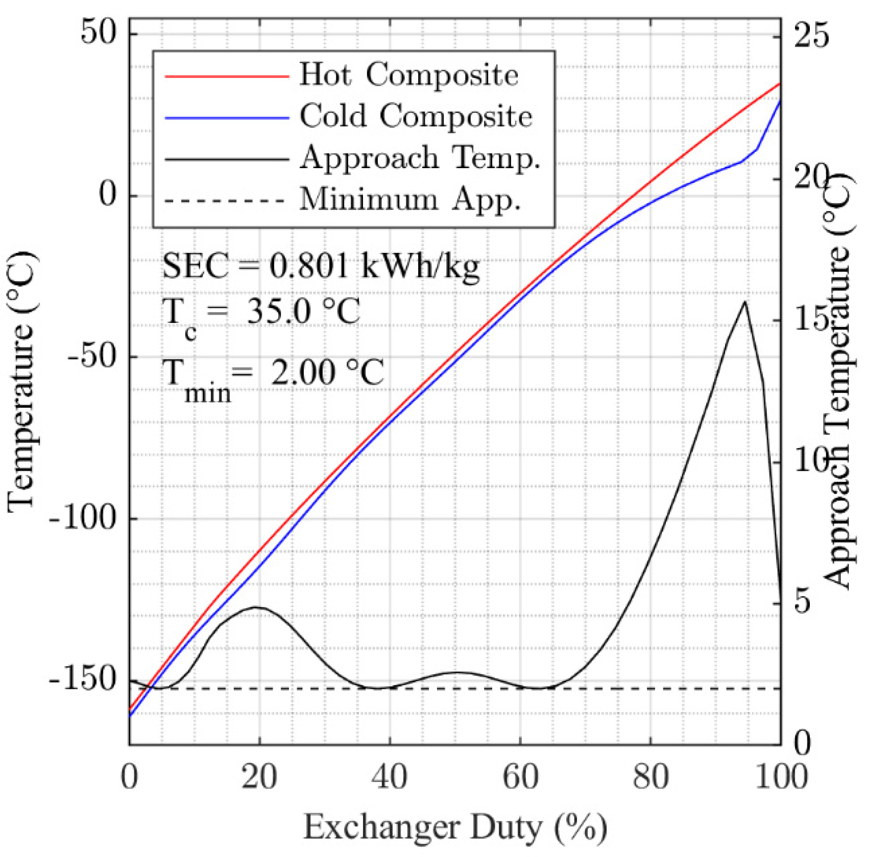
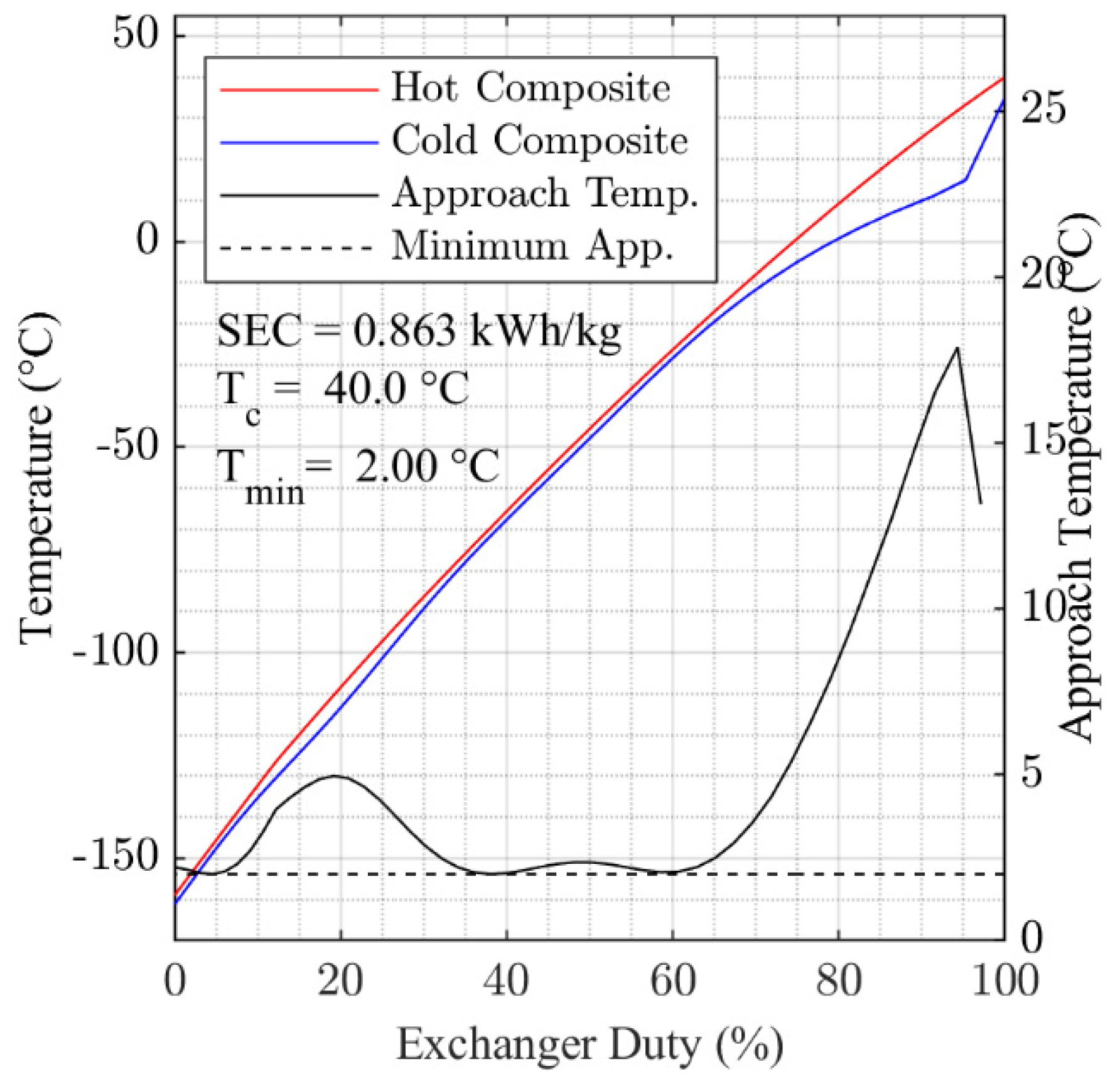
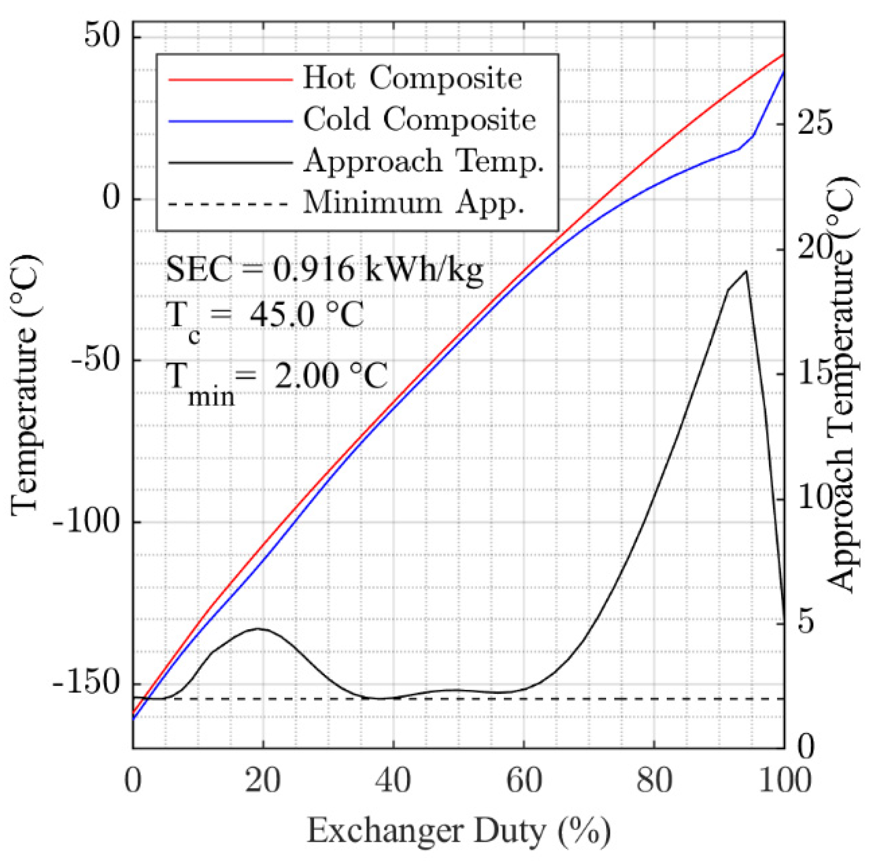
The temperature profiles for the combined hot streams and the cold stream in HX-1—the hot and cold composite curves—were estimated by splitting the heat exchanger into $n$ equally sized temperature intervals, each sized $\left(T_{\mathrm{in}}-T_{\mathrm{out}}\right)/n$ and stream enthalpies calculated for each temperature point ($n+1$, total). Then the heat exchanger duty was also split into $n$ equally sized intervals ($Q_{\mathrm{HX}-1}/n$), and the hot and cold composite temperatures, $T_{\mathrm{HC}}$ and $T_{\mathrm{CC}}$, interpolated at each point ($n+1$, total) using linear interpolation of the temperature-enthalpy data. Finally, the temperature approach was calculated for each point, $∆T=T_{\mathrm{HC}}$ − $T_{\mathrm{CC}}$. In both cases, $n$ was set to 50 to give a high degree of accuracy to the calculations.

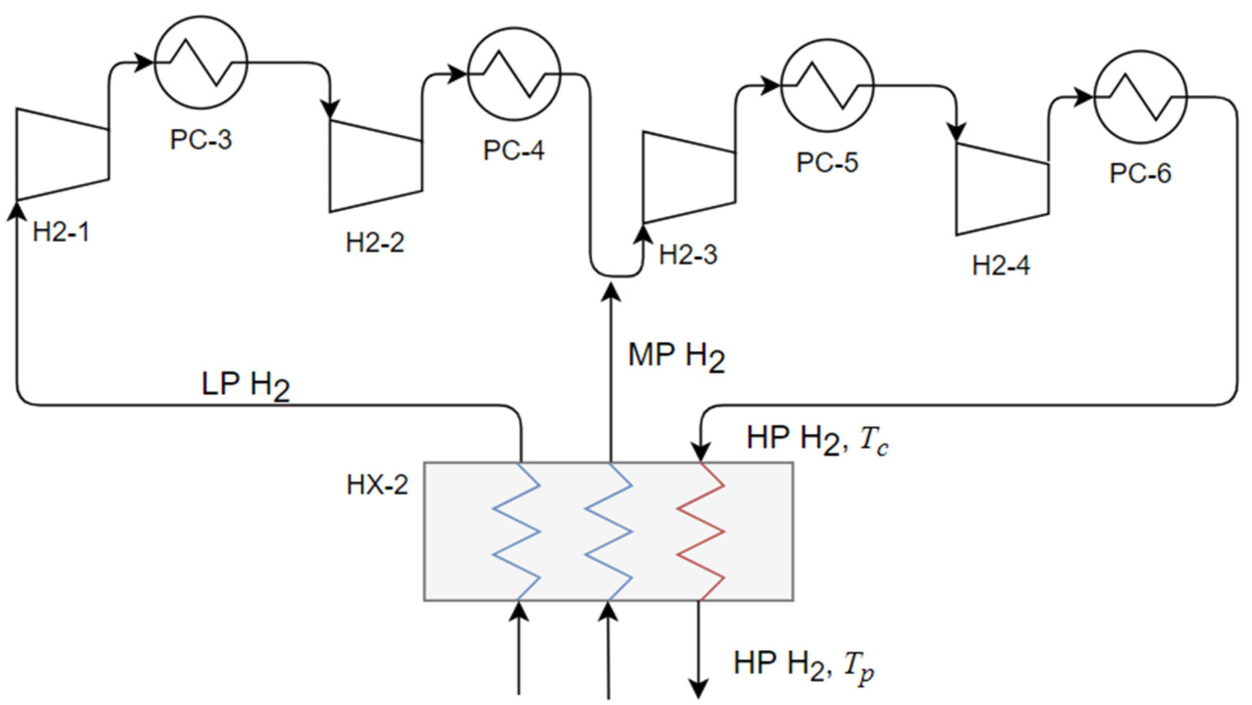
Figure 2 provides a sketch of the cycle compressor (comprising H2-1 to 4) for the cryogenic-cooling step which forms the basis of the present study. The stream LP H₂ represents the low-pressure hydrogen stream returning from the liquefaction process. This stream is compressed in two compressor stages (H2-1 and H2-2) before blending with medium-pressure hydrogen. The combined stream is then compressed in two further compressor stages (H2-3 and H2-4) before being passed-back to a multi-stream heat exchanger (HX-2), which cools the HP stream down to $T_{\mathrm{p}}$. The compressor inter-stage pressures are calculated assuming equal stage pressure ratios.

The model of the cryogen-cooling step compressor shown in Figure 2 was also developed in MATLAB using the same basis as the MR process model.

Table 2. Summary of fixed modelling parameters for the cryogenic-cooling cycle compressor.

Parameter	Value	Units
LP H2 Feed Pressure	1.1	bara
LP H2 flowrate	51.5	tpd
MP H2 feed pressure	8.0	bara
MP H2 flowrate	1121.5	tpd
HP H2 return pressure	29.8	bara
PC-3 to 6 pressure-loss	0.5	bar

Isentropic efficiency.

presents the fixed modelling parameters used in the study performance of this compressor, which are based on the reference model [17]. The outlet temperature of the four after-coolers (PC-3 to 6) were assumed equal to $T_{\mathrm{c}}$ and the inlet temperature of the LP and MP streams to the compressor was assumed to have a 2 °C approach to $T_{\mathrm{c}}$ in all cases.

In addition to the cycle compressor, the reference study describes several turbo-expanders within the cryogenic cooling step. These produce 2.8 MW of shaft power, which is assumed in the reference study to be recovered as electrical energy with as efficiency of 80% [17]. Assuming, as before, that the parameters in the cryogenic process remain constant with varying $T_{\mathrm{c}}$, this recovered energy equates to a specific energy production for the expanders, ${\mathrm{SEC}}_{\mathrm{Ex}}$, of approximately 0.43 kWh/kg, which is a constant value for all cases studied in this work.

Where operating parameters were not available in the reference study, they have been inferred from the data that is presented there. Because of this, it cannot be claimed that there is any direct equivalence between the results presented here and the reference model.

2.3. MR Pre-Cooling Model Validation

An important aspect of successful optimization is the minimization of temperature differences in HX-1, and since the targeted minimum approach temperature is only 1 K, the accuracy of the property predications used in the process model is very important. In the TREND software package, several properties methods are available; to select the basis that is most appropriate for the present work, three of these were compared against results from the reference study: Peng Robinson (PR), Soave-Redlich-Kwong (SRK) and the TREND Helmholtz free energy model.

Table 3. Validation case MR composition.

Component	Mole Fraction
Nitrogen	0.101
Methane	0.324
Ethane	0.274
Propane	0.031
n-Butane	0.270

and

Table 4. Validation case MR modelling parameters.

Parameter	Value	Units
Hydrogen Feed Flow	125	tpd
MR feed temperature	12	°C
MR return temperature	−1.0	°C
MR feed pressure	35	bara
MR return pressure	4.25	bara

present the parameters used in the validation work. The results of the validation work were used to select the properties method used in the later optimization work.

2.4. Optimization Problem Defenition

The objective of the optimization study was to minimize the energy consumption of the MR pre-cooling process whilst satisfying a minimum temperature approach constraint. The objective function was formulated as described in Equation (1):

$$\min \left\{{\mathrm{SEC}}_{\mathrm{MR}}\right\}, \mathrm{such} \mathrm{that} \{\begin{array}{c}{\mathrm{lb}}_i<\mathrm{O}{\mathrm{P}}_i<{\mathrm{lb}}_i\\ ∆T_{\min }-∆T_{\mathrm{acc}}>0\\ {\dot{m}}_{\mathrm{MR}}>0\end{array}.$$

(1)

In Equation (1), ${\mathrm{SEC}}_{\mathrm{MR}}$ is the specific energy consumption of the MR process,${\mathrm{OP}}_i$ are the set of $i$ optimization parameters (see

Table 5. Summary of Optimization Parameters with Initial (${\mathrm{OP}}_{i,0}$) and Constraint Values.

Parameter	Description	$l{b}_{\mathit{i}}<O{P}_{\mathit{i},0}<u{b}_{\mathit{i}}$
${\mathrm{OP}}_1$	MR mole fraction N2	0.05 < 0.11 < 0.25
${\mathrm{OP}}_2$	Mole fraction CH4	0.20 < 0.32 < 0.50
${\mathrm{OP}}_3$	MR mole fraction C2	0.15 < 0.27 < 0.50
${\mathrm{OP}}_4$	MR mole fraction C3	0.00 < 0.03 < 0.10
${\mathrm{OP}}_5$	RC-1, Pin (bara)	2.00 < 4.25 < 6.00

), ${\mathrm{lb}}_i$ and ${\mathrm{ub}}_i$ are a set of lower and upper bounds for each $\mathrm{parameter}$, $∆T_{\min }$ is the minimum approach temperature in HX-1 ($∆T_{\min }=\min \left\{∆T_n\right\}$), $∆T_{\mathrm{acc}}$ is the minimum acceptable approach temperature in HX-1 and ${\dot{m}}_{\mathrm{MR}}$ is the mass flowrate of the MR. ${\mathrm{SEC}}_{\mathrm{MR}}$ was calculated from the sum the compression stage energy consumptions, $W_{\mathrm{MR}}$, which are, in turn, a function of ${\mathrm{OP}}_i$, ${\mathrm{MP}}_i$ (see Table 1) and $T_{\mathrm{c}}$ is described by Equation (2):

$${\mathrm{SEC}}_{\mathrm{MR}}={\displaystyle \sum }{W}_{\mathrm{MR}}\left({\mathrm{OP}}_i,{\mathrm{MP}}_i,T_{\mathrm{c}}\right)/{\dot{m}}_{\mathrm{H}2}.$$

(2)

In Equation (2), ${\dot{m}}_{\mathrm{H}2}$ is the mass flowrate of hydrogen in the pre-cooling process.

The set of optimization parameters, ${\mathrm{OP}}_i$, used in the study are summarized in Table 5 along with the initial values used (${\mathrm{OP}}_{i,0}$) and initial values of the boundary constraints (${\mathrm{lb}}_i$ and ${\mathrm{ub}}_i$).

Although the ultimate purpose of the boundary constraints shown in Table 5 was to limit the optimization process to physically meaningful solutions—e.g., component mole fractions greater than zero—the initial boundary constraints were also used to limit the search area around the likely optimum values. This was done to reduce optimization time. The initial values of lb and ub shown in Table 5 were set based on results from the reference case, but where the optimization solution was found close to the initial limits, the bounds were extended to ensure that the overall optimum solution was not missed.

In addition to the optimization parameters listed in Table 5, the MR compressor inter-stage pressure, MR compressor discharge pressure and HX-1 warm-end approach temperature could be considered as optimization parameters. However, in this work these have been excluded to limit complexity. The MR compressor discharge pressure is, therefore, fixed at the value used in the reference study, the MR inter-stage pressure set in each case to maintain equal stage pressure ratios, and the HX-1 warm-end approach set to 5 °C. The MR mole fraction for butane is also not identified as an optimization parameter because it is calculated from the sum of the other components.

2.5. Optimization Algorithm

In a phase of initial testing the Fmincon (FMC) algorithm with the SQP option was found to provide fast and generally accurate optimization results, although in some cases local minima were found. In all subsequent cases, FMC was used with the solution tolerance set to 0.001 kWh/kg and all other options left as default.

To help identify the global minimum solutions for each $T_{\mathrm{c}}$, the boundary constraints shown in Table 5 were evaluated in a manual, stepwise, process: after the initial results had been gathered, new initial guesses were specified when the original initial guess was found to be a long way from the solution. When a stable set of bounds enclosing the global solution had been found, the MultiStart, MS, and GlobalSearch, GS, algorithms were used to help test the quality of the results. In both cases the MS and GS runs were again based on the FMC algorithm with the parameters as before.

The quality each optimization result was assessed qualitatively using the results from other $T_{\mathrm{c}}$ cases. The basis of this assessment was the assumption that a simple, monotonic, relationship was likely between each of the optimization parameters and $T_{\mathrm{c}}$. In addition to this assessment, the temperature profiles in HX-1 for each case were reviewed qualitatively to determine if $∆T_{\mathrm{acc}}$ was consistently approached throughout the heat exchanger.

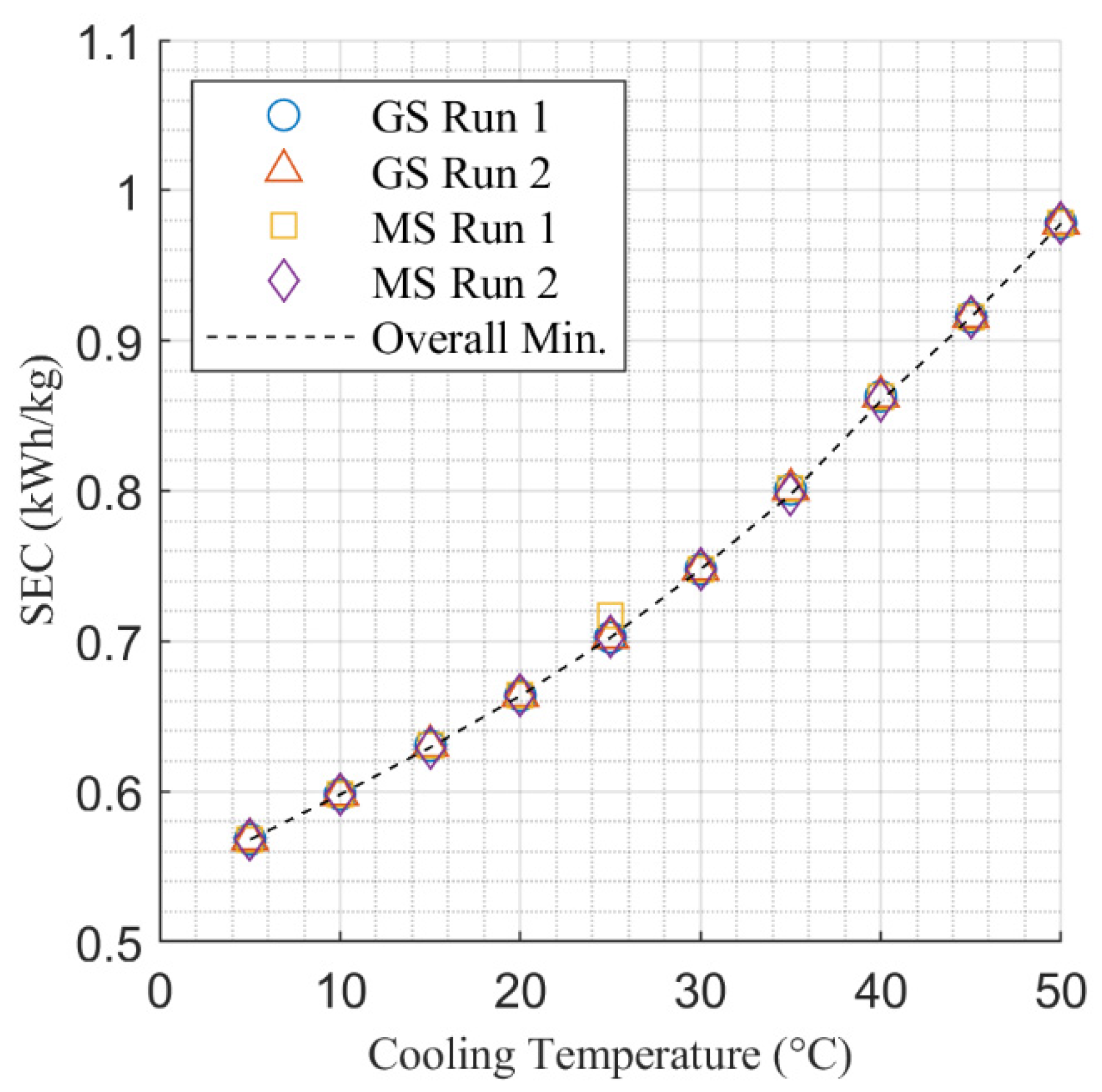
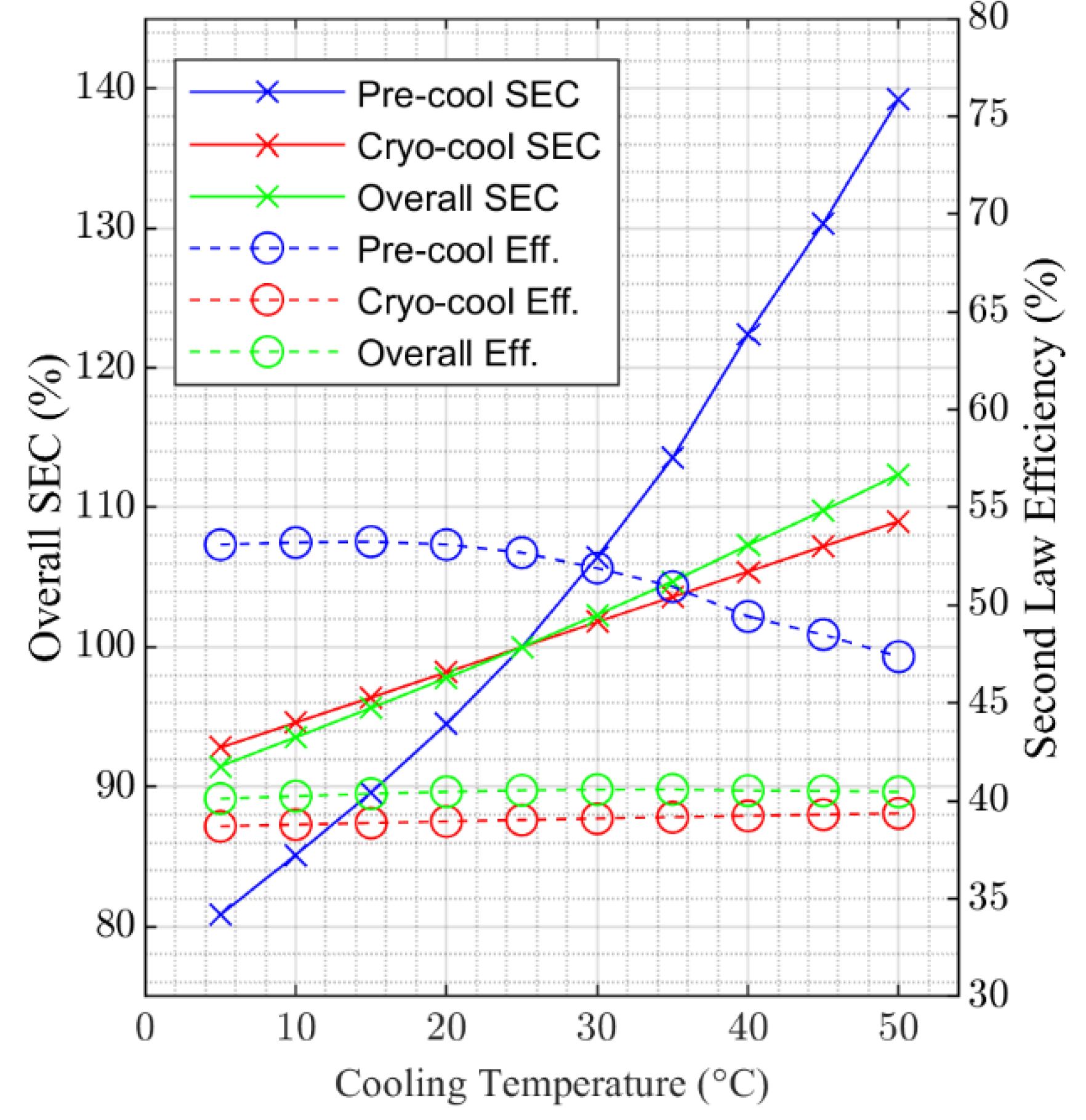
2.6. Performance Variation with Cooling Temperature

Performance variation with cooling temperature was studied for the MR pre-cooling process by finding the optimum operating parameters, ${\mathrm{OP}}_i$, for each cooling temperature, $T_{\mathrm{c}}$ case. The fixed modelling parameters shown in Table 2 were used as the basis in all cases. The cooling temperature range studied was 5 to 50 °C.

In the model developed for the cryogenic-cooling step, process parameters were not optimized: flowrates and pressure levels in the cryogenic cycle were held constant at the values shown in Table 3. The variation of the energy consumption of the cryogenic cycle compressor with $T_c$ was modelled using the more simplistic assumption that, since the composite cooling curves in HX-2 are straight and parallel, a constant warm-end approach temperature exists across the range of cooling temperatures studied. The energy consumption of the cryogenic cycle compressor was calculated using the same basis as that of the MR pre-cooling process. A 2 °C warm-end approach temperature was assumed across the cooling temperature range 5 to 50 °C.

The overall SEC for the hydrogen liquefaction process was calculated as the sum of the energy consumption for the MR pre-cooling step, ${\mathrm{SEC}}_{\mathrm{MR}}$, and the cryogenic-cooling step, ${\mathrm{SEC}}_{\mathrm{CY}},$ which was—in turn—calculated as the sum of the cycle compressor stage energy consumptions minus the energy recovered in the cryogenic-cooling step expanders as described in Equations (3) and (4):

$$\mathrm{SEC}={\mathrm{SEC}}_{\mathrm{MR}}+{\mathrm{SEC}}_{\mathrm{CY}}$$

(3)

$${\mathrm{SEC}}_{\mathrm{CY}}={\displaystyle \sum }{W}_{\mathrm{H}2}\left({\mathrm{MP}}_{\mathrm{H}2},T_c\right)/{\dot{m}}_{\mathrm{H}2}-{\mathrm{SEC}}_{\mathrm{Ex}}$$

(4)

In Equation (3), $W_{\mathrm{H}2}$ is the energy consumption of the cycle compressors shown in Figure 2, and in Equation (4), ${\mathrm{MP}}_{\mathrm{H}2}$ is the set of fixed modelling parameters for the cryogenic-cooling cycle compressor (see Table 2).

To provide an independent means of reviewing the trends shown in the results, the SEC for an ideal process that cooled the hydrogen from $T_{\mathrm{c}}$ to a final temperature of −259 °C was also calculated. This ideal energy consumption, ${\mathrm{SEC}}_{\mathrm{ID}}$, was then used to calculate a second law efficiency, ${\eta }_{\mathrm{id}}=\mathrm{SEC}/ {\mathrm{SEC}}_{\mathrm{ID}}$, for the overall process. The method used to calculate ${\mathrm{SEC}}_{\mathrm{ID}}$ was to summate the ideal Carnot cycle energy consumption for a set of very small temperature steps along temperature–enthalpy data for hydrogen as explained previously by Jackson et al. [29].

3. Results and Discussion

3.1. Process Modelling and Validation

Table 6. Summary of modelling parameters for the model validation work.

	Reference	Case A	Case B	Case C
Properties method	-	PR	SRK	Hel.
MP supply pressure	35.0	35.0	35.0	35.0	bara
MR return pressure	4.25	3.0 **	4.25	4.25	bara
MR return temp.	112	112.8	112.3	109.6	°C
MR mass flowrate	1600 *	1395	1703	1709	tpd
HX-1 min. approach	1.00	1.05	0.49	0.51	°C
HX-1 duty	12.6	11.2	13.2	12.9	kW

* Given only as an approximate value in the reference case. ** Adjusted to give a positive value for min. approach.

shows the results from the model validation work. In addition to the results from the reference study, three sets of results are presented in Table 6: Case A uses the TREND implementation of the Peng Robinson (PR) equation of state; Case B the TREND/SRK equation of state; and Case C the TREND/ Helmholtz free energy properties method.

Of the three cases compared in Table 6, Case C—using the TREND/ Helmholtz free energy properties method—is considered to represent the closest match to the reference case, but since Case B also offers good agreement and significantly reduced calculation time, SRK is selected as the basis for further work.

Figure 3 presents the composite temperature profile data for Case B and C in Table 6. The results show that, although the shape of the curves differs between the two cases, the results from both cases show a very good fit between the warm and cold curves throughout the heat exchanger. These results, therefore, add confidence to the validation work and the selection of Case B as the modelling basis.

While Table 6 and Figure 3 show that the selection of a good modelling basis is important to the determination of the optimum operating parameters for this process, no claim is made here that the modelling basis selected is the one that is most accurate for the modelling of this process, just that it provided a good match with the reference case in the validation work presented.

A limitation of the present study is that the heat generated during ortho-para hydrogen conversion is omitted form the model. This is a simplification that limits the extent to which this modelling work reflects the performance of a hydrogen liquefaction process operating in the real world. The main claim made here regarding the modelling basis is that it provides provide a consistent basis to study performance across the operating cases considered. The implication of this for further work is that the study of the variation in energy consumption with cooling temperature made here is valid and can provide some insight into how the performance real hydrogen liquefaction processes can be expected to vary when designed for utility cooling at different temperatures.

3.2. Performance Variation with Cooling Temperature

Figure 4 and Figure 5 show how the five optimization parameters vary with $T_{\mathrm{c}}$, and Figure 6 and Figure 7 provide two examples of the optimized cooling curves resulting from these runs. In Figure 4 and Figure 5 all of the data collected over the final set of optimization runs (two using GS and two using MS) are presented as points and the overall optimum datasets are connected by dotted lines.

The results presented in Figure 4 for MR composition show quite clear trends with the component mole fraction of each component a monotonic function of cooling temperature in the majority of cases. The impact on butane is largest, which is due to the steadily increasing heat duty at the warm end of HX-1 as the cooling temperature increases. The impact on the optimum nitrogen content in the MR is affected least by cooling temperature, reflecting the relatively static conditions at the cold end of HX-1.

The data presented in Figure 4 that represents optimum MR pressure solutions is less consistent with a slight upward trend visible across the range of cooling temperatures considered. This indicates that the optimum combination of MR composition and MR operating pressure is more difficult to determine and that the overall minimum may not have been found in all cases. However, Figure 5 shows a very consistent trend in how the SEC for the MR pre-cooling process varies with $T_{\mathrm{c}}$, which provides confidence that a solution close to the overall minimum was found in all cases.

Figure 6 and Figure 7 present the hot and cold composite cooling curves for the overall minimum SEC solutions found for $T_{\mathrm{c}}$ = 5 °C and $T_{\mathrm{c}}$ = 50 °C. Generally, the results in Figure 6 and Figure 7 show that the optimization algorithm has found a good fit for the cooling curves, with the 2 °C pinch temperature approached in multiple locations within HX-1 in both cases. The cooling curves for each of the temperature points studied between $T_{\mathrm{c}}$ = 5 °C and $T_{\mathrm{c}}$ = 50 °C are presented in Figure A2, Figure A3, Figure A4, Figure A5, Figure A6, Figure A7, Figure A8 and Figure A9, which are contained in the Appendix A.

Comparing the variation in minimum approach temperature data presented in Figure 6 for $T_{\mathrm{c}}$ = 5 °C with that presented in Figure 7 for $T_{\mathrm{c}}$ = 50 °C, it can also be observed that the optimization process has found a set of parameters that better minimize the temperature approach in HX-1 for the $T_{\mathrm{c}}$ = 5 °C case. Looking at the $T_{\mathrm{c}}$ = 50 °C case, we see that it becomes more difficult to maintain a close approach at the warm end of the heat exchanger suggesting that SEC could be reduced further through the addition of heavier components to the MR.

Figure 8 presents the SEC for the pre-cooling step, the cryogenic-cooling step, and the overall process. Figure 9 presents the same data in terms of the % change relative to the 25 °C case. Moreover, presented in Figure 9 are the corresponding second law efficiencies expressed as a percentage.

Figure 8 shows that the contribution of the pre-cooling process to overall SEC across the range of cooling temperatures investigated is approximately 10%. In addition, Figure 8 shows non-linear variation in SEC with cooling temperature for the pre-cooling part of the overall process that contrasts with the linear relationship between SEC and cooling temperature for the cryogenic process. This non-linear relationship for the pre-cooling process reflects the fact that lower cooling temperatures both reduced cooling duty and increase efficiency, whereas the close to linear impact on the cryogenic process is a result of only reduced increased efficiency. Further insight into this is provided by the results presented in Figure 9.

The results presented in Figure 9 show that energy consumption for the overall liquefaction process increases by around 20% across the cooling temperature range 5 to 50 °C and 5% over the range 20 to 30 °C. For the pre-cooling process the increase is close to 80% over the full temperature range. Figure 9 also shows that while the second law efficiency of the cryogenic-cooling process increases slightly across the range of temperatures considered, the efficiency of the pre-cooling process drops above 25 °C. The cause of this drop in efficiency as the cooling temperature increases can be seen in Figure 6 and Figure 7, which show that the mean temperature approach for the higher temperature cases is higher than that of the lower temperature cases. It is this reduced level of optimization as cooling temperature increases above 25 °C that accentuates the non-linear behavior notable in Figure 8.

The implication of the results presented in Figure 9 is the same as discussed earlier: that design changes in the MR process could help to improve performance for the cases where the cooling temperature is higher than 25 °C. Both the addition of heavier components to the MR mixture could provide a more optimized design or the division of the MR loop into additional pressure levels. Both of these design alternatives could form the basis of further study work.

4. Conclusions

A model for a hydrogen liquefaction process has been developed and validated against results from an independent study. Although the validation process highlighted the significant impact that different properties models can have on model predictions, the validation results also indicate that the present model is suitable for the study of the impact of ambient temperature on process performance.

A set of optimization parameters were selected, and an optimization method developed that was shown to be suitable for the study of process performance across a range of process cooling temperatures through the consistency of the results obtained. The MR studied is limited to a mixture of five components. It is indicated in the results presented that the addition of heavier components could be used to improve efficiency for cooling temperatures above 25 °C, although the available gains would be small.

The results of the optimization work show that the specific energy consumption, SEC, of the MR pre-cooling process increases by around 80%, from approximately 0.57 to 1.0 kWh/kg, across the cooling temperature range 5 to 50 °C. These results, combined with the calculated process performance for the cryogenic-cooling step (not optimized here), show that total energy consumption for the hydrogen liquefaction process increases by around 20%, from 5.8 to 7.1 kWh/kg, across the same temperature range. Considering just the range 20 to 30 °C, there is a 5% increase, which illustrates the significant impact ambient temperature can have on energy consumption.

The variation in energy consumption with cooling temperature implies a significant benefit for liquefaction processes operating in low ambient temperature locations, especially given that the hydrogen liquefaction process represents a very energy intensive step in the supply of liquid hydrogen. The aim of further work is to combine these results into a larger system model that considers the impact of ambient temperature on the supply of low-carbon energy from natural gas.

References

1. Acar, C.; Dincer, I. Review and evaluation of hydrogen production options for better environment. J. Clean. Prod. 2019, 218, 835–849. [Google Scholar] [CrossRef]
2. Cell, F.; Undertaking, H.J. Hydrogen Roadmap Europe—A Sustainable Pathway for the European Energy Transition. Fuel Cells Hydrogen Jt. Undert. 2019. [Google Scholar] [CrossRef]
3. Moya, J.I.; Dalius, W. Hydrogen Use in EU Decarbonisation Scenarios. Available online: https://ec.europa.eu/jrc/sites/default/files/final_insights_into_hydrogen_use_public_version.pdf (accessed on 1 September 2021).
4. The European Comission. A Hydrogen Strategy for a Climate-Neutral Europe; The European Comission: Brussels, Belgium, 2020. [Google Scholar]
5. Kang, J.-N.; Wei, Y.-M.; Liu, L.-C.; Han, R.; Yu, B.-Y.; Wang, J.-W. Energy systems for climate change mitigation: A systematic review. Appl. Energy 2020, 263, 114602. [Google Scholar] [CrossRef]
6. Yuksel, Y.E.; Ozturk, M.; Dincer, I. Energetic and exergetic assessments of a novel solar power tower based multigeneration system with hydrogen production and liquefaction. Int. J. Hydrogen Energy 2019, 44, 13071–13084. [Google Scholar] [CrossRef]
7. Sher, F.; Al-Shara, N.K.; Iqbal, S.Z.; Jahan, Z.; Chen, G.Z. Enhancing hydrogen production from steam electrolysis in molten hydroxides via selection of non-precious metal electrodes. Int. J. Hydrogen Energy 2020, 45, 28260–28271. [Google Scholar] [CrossRef]
8. Karakaya, E.; Nuur, C.; Assbring, L. Potential transitions in the iron and steel industry in Sweden: Towards a hydrogen-based future? J. Clean. Prod. 2018, 195, 651–663. [Google Scholar] [CrossRef]
9. Pethaiah, S.S.; Sadasivuni, K.K.; Jayakumar, A.; Ponnamma, D.; Tiwary, C.S.; Sasikumar, G. Methanol Electrolysis for Hydrogen Production Using Polymer Electrolyte Membrane: A Mini-Review. Energies 2020, 13, 5879. [Google Scholar] [CrossRef]
10. Yang, C.; Ogden, J. Determining the lowest-cost hydrogen delivery mode. Int. J. Hydrogen Energy 2007, 32, 268–286. [Google Scholar] [CrossRef] [Green Version]
11. Ishimoto, Y.; Voldsund, M.; Nekså, P.; Roussanaly, S.; Berstad, D.; Gardarsdottir, S.O. Large-scale production and transport of hydrogen from Norway to Europe and Japan: Value chain analysis and comparison of liquid hydrogen and ammonia as energy carriers. Int. J. Hydrogen Energy 2020, 45, 32865–32883. [Google Scholar] [CrossRef]
12. Hoshi, M. World’s First Liquid Hydrogen Carrier Ship Launches in Japan. Available online: https://asia.nikkei.com/Business/Energy/World-s-first-liquid-hydrogen-carrier-ship-launches-in-Japan (accessed on 15 April 2021).
13. Aasadnia, M.; Mehrpooya, M. Large-scale liquid hydrogen production methods and approaches: A review. Appl. Energy 2018, 212, 57–83. [Google Scholar] [CrossRef]
14. Ghorbani, B.; Mehrpooya, M.; Aasadnia, M.; Niasar, M.S. Hydrogen liquefaction process using solar energy and organic Rankine cycle power system. J. Clean. Prod. 2019, 235, 1465–1482. [Google Scholar] [CrossRef]
15. Yilmaz, C. Optimum energy evaluation and life cycle cost assessment of a hydrogen liquefaction system assisted by geothermal energy. Int. J. Hydrogen Energy 2019, 45, 3558–3568. [Google Scholar] [CrossRef]
16. Ansarinasab, H.; Mehrpooya, M.; Mohammadi, A. Advanced exergy and exergoeconomic analyses of a hydrogen liquefaction plant equipped with mixed refrigerant system. J. Clean. Prod. 2017, 144, 248–259. [Google Scholar] [CrossRef]
17. Skaugen, G.; Berstad, D.; Wilhelmsen, Ø. Comparing exergy losses and evaluating the potential of catalyst-filled plate-fin and spiral-wound heat exchangers in a large-scale Claude hydrogen liquefaction process. Int. J. Hydrogen Energy 2020, 45, 6663–6679. [Google Scholar] [CrossRef]
18. Cardella, U.; Decker, L.; Sundberg, J.; Klein, H. Process optimization for large-scale hydrogen liquefaction. Int. J. Hydrogen Energy 2017, 42, 12339–12354. [Google Scholar] [CrossRef]
19. Yuksel, Y.E.; Ozturk, M.; Dincer, I. Analysis and assessment of a novel hydrogen liquefaction process. Int. J. Hydrogen Energy 2017, 42, 11429–11438. [Google Scholar] [CrossRef]
20. Chang, H.M.; Ryu, K.N.; Baik, J.H. Thermodynamic design of hydrogen liquefaction systems with helium or neon Brayton refrigerator. Cryogenics 2018, 91, 68–76. [Google Scholar] [CrossRef]
21. Donaubauer, P.J.; Cardella, U.; Decker, L.; Klein, H. Kinetics and Heat Exchanger Design for Catalytic Ortho-Para Hydrogen Conversion during Liquefaction. Chem. Eng. Technol. 2019, 42, 669–679. [Google Scholar] [CrossRef]
22. Wilhelmsen, O.; Berstad, D.; Aasen, A.; Neksa, P.; Skaugen, G. Reducing the exergy destruction in the cryogenic heat exchangers of hydrogen liquefaction processes. Int. J. Hydrogen Energy 2018, 43, 5033–5047. [Google Scholar] [CrossRef] [Green Version]
23. Skaugen, G.; Wilhelmsen, O. Comparing the Performance of Plate-Fin and Spiral Wound Heat Exchangers in the Cryogenic Part of the Hydrogen Liquefaction Process. In Proceedings of the 15th Cryogenics 2019 Iir International Conference; Prague, Czech Republic, 8–11 April 2019, Chrz, V., Haberstroh, C., Herzog, R., Kaiser, Z., Klier, J., Kralik, T., Lansky, M., Mericka, P., Schustr, P., Srnka, A., et al., Eds.; Refrigeration Science and Technology; International Institute of Refrigeration: Paris, France, 2019; pp. 318–324. [Google Scholar]
24. Bauer, H.C. Mixed fluid cascade, experience and outlook. In Proceedings of the AIChE Spring Meeting and Global Congress on Process Safety, Houston, TX, USA, 1–4 April 2012. [Google Scholar]
25. Rian, A.B.; Ertesvåg, I.S. Exergy Evaluation of the Arctic Snøhvit Liquefied Natural Gas Processing Plant in Northern Norway—Significance of Ambient Temperature. Energy Fuels 2012, 26, 1259–1267. [Google Scholar] [CrossRef]
26. Xu, X.; Liu, J.; Jiang, C.; Cao, L. The correlation between mixed refrigerant composition and ambient conditions in the PRICO LNG process. Appl. Energy 2013, 102, 1127–1136. [Google Scholar] [CrossRef]
27. Castillo, L.; Dahouk Majzoub, M.; Di Scipio, S.; Dorao, C.A. Conceptual analysis of the precooling stage for LNG processes. Energy Convers. Manag. 2013, 66, 41–47. [Google Scholar] [CrossRef]
28. Park, K.; Won, W.; Shin, D. Effects of varying the ambient temperature on the performance of a single mixed refrigerant liquefaction process. J. Nat. Gas Sci. Eng. 2016, 34, 958–968. [Google Scholar] [CrossRef]
29. Jackson, S.; Eiksund, O.; Brodal, E. Impact of Ambient Temperature on LNG Liquefaction Process Performance: Energy Efficiency and CO 2 Emissions in Cold Climates. Ind. Eng. Chem. Res. 2017, 56, 3388–3398. [Google Scholar] [CrossRef]
30. Cardella, U.; Decker, L.; Klein, H. Roadmap to economically viable hydrogen liquefaction. Int. J. Hydrogen Energy 2017, 42, 13329–13338. [Google Scholar] [CrossRef]
31. The MathWorks, Inc. MATLAB; The MathWorks, Inc.: Natick, MA, USA, 2018. [Google Scholar]
32. Span, R.; Eckermann, T.; Herrig, S.; Hielscher, S.; Jäger, A.; Thol, M. TREND. Thermodynamic Reference and Engineering Data 5.0; Lehrstuhl für Thermodynamik, Ruhr-Universität Bochum: Bochum, Germany, 2020. [Google Scholar]
Figure 1. Flow diagram for the MR H2 pre-cooling process.
Energies 14 06090 g001
Figure 2. Flow diagram of the cryogenic-cooling step H2 cycle compressor.
Energies 14 06090 g002
Figure 3. Composite Curves and Key Performance Parameters for HX-1, MR Pre-cooling Process: (a) Case B; (b) Case C.
Energies 14 06090 g003
Figure 4. Variation in OP for the MR pre-cooling step with cooling temperature.
Energies 14 06090 g004
Figure 5. Variation in SEC for the MR pre-cooling step with cooling temperature.
Energies 14 06090 g005
Figure 6. Composite curves in HX-1 and key performance parameters, 5 °C cooling temperature case.
Energies 14 06090 g006
Figure 7. Composite curves in HX-1 and key performance parameters, 50 °C cooling temperature case.
Energies 14 06090 g007
Figure 8. Variation in SEC with cooling temperature for the pre-cooling, cryogenic-cooling and overall cooling processes.
Energies 14 06090 g008
Figure 9. Percentage variation in overall SEC and second law efficiency for the pre-cooling, cryogenic-cooling and overall cooling processes.
Energies 14 06090 g009