Model-Based Range Prediction for Electric Cars and Trucks under Real-World Conditions

Abstract

The further development of electric mobility requires major scientific efforts to obtain reliable data for vehicle and drive development. Practical experience has repeatedly shown that vehicle data sheets do not contain realistic consumption and range figures. Since the fear of low range is a significant obstacle to the acceptance of electric mobility, a reliable database can provide developers with additional insights and create confidence among vehicle users. This study presents a detailed, yet easy-to-implement and modular physical model for both passenger and commercial battery electric vehicles. The model takes consumption-relevant parameters, such as seasonal influences, terrain character, and driving behavior, into account. Without any a posteriori parameter adjustments, an excellent agreement with known field data and other experimental observations is achieved. This validation conveys much credibility to model predictions regarding the real-world impact on energy consumption and cruising range in standardized driving cycles. Some of the conclusions, almost impossible to obtain experimentally, are that winter conditions and a hilly terrain each reduce the range by 7–9%, and aggressive driving reduces the range by up to 20%. The quantitative results also reveal the important contributions of recuperation and rolling resistance towards the overall energy budget.

1. Introduction

Type approvals of technical devices are usually based on standardized test procedures to ensure that the results are repeatable and that the performance of different devices can be compared on the basis of the test results. A conformity test evaluates if a device meets stipulated requirements under test conditions. This does not necessarily allow conclusions about the device behavior in the real world.

A case in point is the type approval of vehicles. Standard test cycles serve to determine the energy consumption and emission levels of vehicles. For example, the New European Driving Cycle (NEDC) was devised to characterize internal combustion engine vehicles (ICEVs)—but only passenger cars, no light trucks or commercial vehicles—and was later also used to characterize the energy consumption and driving range of battery electric vehicles (BEVs) [1]. The test is performed with an idealized driving speed pattern on a roller test bench. Aerodynamic drag and inertial forces, which would slow down the vehicle on the road, are emulated by an electrical machine, and a fan provides the airflow the vehicle air intakes would see at a given speed [1].

Numerous factors that increase the energy consumption are ignored on the test bench. The vehicle is tested with minimum payload; ancillary loads, such as lights, air-conditioning, or window heating, are turned off; weather conditions, such as wind, rain, and high or low temperatures, are ignored; tires are inflated to pressures above recommended values; the test can be conducted at 2 km/h below the required speed; the final test results can be arbitrarily reduced by 4%; road inclination and curves are not emulated; etc. For this reason, and also because the gentle test speed pattern does not reflect actual driving habits, the energy consumption and—for ICEVs—the emissions of a vehicle on the road exceed NEDC-based manufacturer specifications [2].

The difference can be significant. Hao et al. find that the actual electricity consumption of BEVs exceeds NEDC test values by 7–10% [3]. For ICEVs, Ma et al. report a real-world energy consumption up to 37.5% higher than NEDC test values [4]. The difference has increased with time and, in some cases, now exceeds 50%. This explains why the overall gas and diesel consumption of a country such as Germany is significantly above the quantities one would expect with car manufacturer specifications [5].

In Europe, the NEDC was replaced in 2018 by the more severe and realistic Worldwide Harmonized Light Vehicles Test Procedure (WLTP) cycle [6]. More realistic operational conditions are also offered by the Artemis cycle [7]. Laurikko et al. measured a grid energy uptake (in kWh/km) of a BEV running through the Artemis Motorway cycle at an ambient temperature of −20 °C, which was 133% above the value of the vehicle running through the NEDC at +23 °C [8].

In order to be able to fully control the test conditions and to allow a later comparison with model calculations, we performed our own road tests with three up-to-date BEV models. The trips took place in the hilly region of Northern Bavaria in Germany in late autumn or early winter. The driver was always the same, and he drove as he was used to with an ICEV. The courses included approximately equal proportions of urban traffic, rural roads, and motorways. The results are documented in detail in Appendix A 

Table A1. Details of roundtrips with three BEVs.

Item	Road Test No.
	1	2	3
BEV type	Renault Zoe	Volkswagen ID3	Tesla Model 3
Battery capacity/kWh	50	58	75
Trip details
Start and end point	Bayreuth, Germany	Hof, Germany	Nürnberg, Germany
Date	24 November 2020	29 October 2020	3 November 2020
Starting time	9:15 a.m.	8:45 a.m.	10:15 a.m.
Duration/min	60	56	82
Temperature at start/°C	1	8	11
Length of trip/km	55.9	49.1	80.5
Average speed/km/h	55.9	52.6	58.9
Altitude above normal zero/m	340	510	309
Travel section
in urban area/km	13.8 (24.6%)	9.6 (19.6%)	16.4 (20.4%)
in rural area/km	24.4 (43.7%)	29.8 (60.7%)	45.3 (56.3%)
on motorway/km	17.7 (31.7%)	9.7 (19.8%)	18.8 (23.4%)
Results–specific consumption
Test result/(kWh/km)	0.215	0.263	0.242
Data sheet value/(kWh/km)	0.172	0.138	0.129
Vehicle range
Test result/km *	233	220	310
Data sheet value/km	291	400	580

* The range is calculated from the nominal capacity (kWh) of the car battery divided by the determined specific consumption (kWh/km).

. They fully confirm the expectations and the results of the cited literature (see

Table 1. Results of own BEV consumption tests under real-world conditions with predicted range (for details, see Table A1).

Vehicle	Range/km		Deviation/%
	Test Result	Data Sheet
Renault ZOE	233	291	−19.9
VW ID 3	220	400	−45.0
Tesla Model 3	310	580	−46.6

) [3,4,5,8]. These data do not represent statistical deviations. Cruising ranges in the field are always significantly lower than the manufacturers’ data-sheet values.

As useful as standard test procedures may be in terms of repeatability and comparability, they obviously are no reliable basis for predicting the energy consumption on the road or the vehicle range.

It was the aim of this study to find a method to predict the real-world electricity consumption of BEVs, both cars and trucks, that meets the following requirements:

• Capability to judge how close standardized test procedures are to reality.
• Suitability for sensitivity analyses with respect to the following:

  (a)

  Technology details (battery weight, battery efficiency, tire rolling resistance, etc.);

  (b)

  Temperature (weather, self-heating);

  (c)

  Terrain characteristics (road inclination);

  (d)

  Driving attitudes (passive, standard, or aggressive).

• Only a priori simulations with physically or technically determined parameters, no a posteriori parameter adjustments to make results better, agree with independent data.

The underlying motivation for this work is the desire to evaluate current and future mobility and sector coupling concepts. Any such concept is based on technical and economic assumptions and has ecological consequences, and we would like to shed more light on the dependencies involved.

The desired consumption prediction is best achieved with a model-based strategy. This is justified in Section 2. In Section 3, we describe our model and its salient features. Section 4 presents sample results meant to validate the model and application results, together with conclusions.

2. Methodology of Real-World Energy Consumption Predictions

The dynamic estimation of the remaining range of a given BEV on the road must take into account the current state of the vehicle (speed, acceleration, tire pressure, state of charge (SoC), and state of health (SoH) of the battery, energy consumption of ancillary loads, etc.) and its environment (road type, road inclination, traffic conditions, headwind or tailwind, temperature, etc.). A driver on the road is interested in this individual range estimation and cannot do anything with the average range of the average car under average conditions.

The average range, however, is of substantial interest for society as a whole. Headwind and tailwind will occur equally often in reality, so the wind influence need not be considered when one is interested in the electricity consumption of large vehicle fleets. On the other hand, ancillary loads will not all be turned off in reality, so their influence on electricity consumption must be taken into account when one is interested in the electricity consumption of large vehicle fleets. The same holds true for the influence of engine efficiency, battery weight, road type, temperature, etc.

In our work, we are concerned with average or typical vehicles and driving conditions in Germany and similar regions. An outside temperature of 25 °C and straight flat roads are not typical then. An electrical machine peak efficiency of 90% may be typical today (exceeded by some motors, not reached by others) and rare (exceeded by most motors) in 30 years.

The comparison of mobility and sector coupling concepts obviously allows complexity-reduction strategies. Everything that has an impact on the current or future average energy consumption must be considered. All specifics buried in the statistical noise of large vehicle fleets can be disregarded.

The desired method for predicting the real-world energy consumption of vehicles can be developed by experimental or by model-based strategies.

2.1. Experimental Approaches

The energy consumption of a vehicle is observable experimentally on a test bench or on the road. In both cases, one can construct statistical models. Test cycles, of course, yield unrealistic results when the test conditions are unrealistic [2]. A model-free, purely statistical evaluation of real-world measurements can be useful for range calculations when road type and average energy consumption can be linked to one another [9]. The calculation is improved by taking into account at least some external parameters, e.g., the road inclination, and some details of the vehicle dynamics [10]. The better the vehicle state and the driving situation are taken into account, the better the prediction quality [11]. Such experimental approaches have been used successfully to quantify the difference between type approval characteristics and road characteristics of vehicles [3,4,5]. They have also been used together with statistical models to draw conclusions on failure probabilities as a function of driving range [12].

However, such statistical models suffer from two drawbacks. First, they only describe the tested vehicles under test conditions. The transferability of the results to other vehicle types or conditions is unclear. Secondly, there is no invertible link between a statistical detail and the underlying physics. Statistics cannot answer questions such as the following: “What would be the consequences if the electrical machine efficiency increased from 85 to 92%?”

2.2. Model-Based Approaches

Nowadays, powerful tools for the simulation of vehicle drivelines are available. May it suffice to mention Matlab with Simscape Driveline or Powertrain Blockset by Mathworks, which offers pre-built, but customizable vehicle models [13]; Cruise by AVL List, a vehicle driveline simulation solution that enables the analysis of electrified powertrain concepts [14,15]; and GT-Suite by Gamma Technologies, a CAE platform for multi-physics system simulations [16]. These tools are indispensable if a specific vehicle is to be designed. They contain numerous physical details which are important for the vehicle dynamics [17]. On a continuous scale from physics-free statistics at the left end to full consideration of all physical details at the right end, purely statistical–experimental methods are too far left for our purposes, and the tools just discussed are too close to the right. The center of the scale is just about right, allowing conclusions about the impact of energy-relevant design parameters and not requiring too many design details. This can only be achieved by model-based concepts similar to functional diagrams known from control theory. The functional blocks in the diagram describe the functional relationship between input and output variables without having to unnecessarily include many details. In the following, we describe such a model. Although simple enough, all of its parameters can be traced back to physical origins.

3. Model Description

When evaluating the impact of transportation solutions on the level of whole societies, one must take all relevant vehicle classes into account. Data on trucks are rare in the literature, although this vehicle class contributes considerably to greenhouse gas emissions. Our objective therefore was to develop a modular simulation model that can be applied to different vehicle classes. To avoid manufacturer and type dependencies, four generic vehicle classes were defined (

Table 2. Definition of vehicle classes. For further parameters, see Appendix B.

Vehicle Class	Rated Motor Power/kW	Total Weight/t	Battery Capacity/kWh
Small car	80	1.6	60
Big car	120	2.0	90
Small truck	160	14.7	120
Big truck	500	24.0	500

).

The suitability of electric drives for small passenger vehicles in urban traffic is undisputed. However, emerging drive technologies must also be able to provide answers for other areas of road transport. While battery-powered electric drive technology is already on its way to drive small trucks used in regional logistics, it is by no means clear whether the battery will be suitable as an energy storage device for transporting large loads over long distances. On the other hand, there is much to suggest that the electric motor in combination with the H₂ fuel-cell and an appropriate tank could become more relevant for heavy trucks [18,19]. We therefore considered three generic drive technologies in our model platform (

Table 3. Major drive and energy storage technologies used in the simulation model.

Drive	Energy Storage
Electric motor	Battery
Electric motor	H2 fuel-cell with tank and battery
ICEV running on compressed natural gas (CNG)	CNG tank

). The CNG engine is commonly regarded as a bridging technology with no long-term perspective because of its comparatively low combustion efficiency and its high CO₂ emissions [19,20]. We included it as a quickly available benchmark for big trucks.

In the following, we limit ourselves to small cars and small trucks, as sufficient empirical data are already available for these vehicle classes [21,22,23] which allow us to independently validate the model predictions. This validation of consumption and range predictions is all the more important because they provide confidence in the reliability of other predictions that cannot be tested experimentally. Such a lack of experimental testability occurs in particular when statements are to be made about larger vehicle fleets or about future developments.

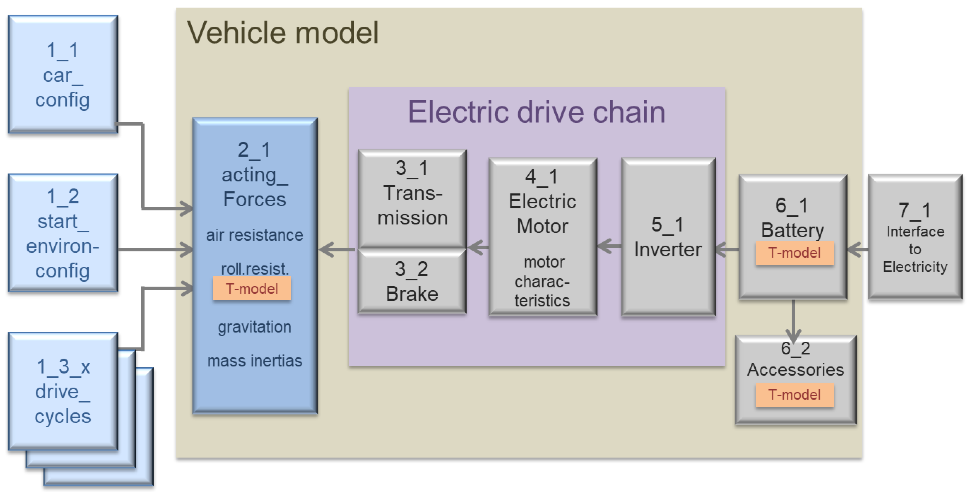
A schematic block diagram of the modular vehicle model is shown in Figure 1. The basic building blocks describe the physics, the drive technology, and the chemistry of the battery either by exact analytical equations or by functional approximations. In order to represent the main temperature influences, suitable temperature models were provided for the rolling resistance of the tires, the battery, and the accessories. The following subsections describe the equations behind the functional elements of the block diagram. The entire model was implemented in Microsoft Excel to exploit the easy availability and intuitive user interface of this software.

3.1. Acting Forces

3.1.1. Air Resistance

The air resistance opposing the motion of the vehicle is described by the drag equation:

$$F_w=\frac{1}{2}{c}_{w}A\rho v^2$$

(1)

where $c_w$ is the dimensionless drag coefficient, $A$ the effective cross-section of the vehicle, $\rho$ the mass density of air, and $v$ the velocity of the vehicle. Moreover, $\rho$ depends on humidity, temperature, and altitude. The latter parameter is important for the terrain influence on energy consumption. We model it by the international altitude formula for air pressure, which gives a better approximation to real-world experimental data near the surface of the earth than the barometric altitude formula [24], where h is the altitude over normal zero and h₀ is the normal zero (in our case the referential altitude in Germany):

$$\rho \left(h\right)=\rho \left(h_0\right)·{\left(1-2.256\times {10}^{-5}{\mathrm{m}}^{-1}·\left(h-h_0\right)\right)}^{5.255}.$$

(2)

We considered both flat and hilly terrains in our simulations and could see that differences in altitude and their effect on $\rho$ played a non-negligible role. In contrast, the temperature influence on $\rho$ was not taken into account, as it only has a small indirect effect on the results.

For the numerical values of the various parameters, see

Table A2. Vehicle parameters used for state-of-the-art BEVs.

Parameter	Vehicle Class
	Small Car	Small Truck
Weight/kg
Empty vehicle	1183	2247
Battery	300	600
Driver + Co	112.5	75
Payload	25	1750
Total	1610	4672
Air resistance
Drag coefficient $c_w$	0.2	0.325
Effective cross-section $A$/m2	2.2	4.5
Rolling resistance
Number of wheels	4	4
Rolling resistance coefficient $C_{\mathrm{r}}$/10−2
on asphalt	1.2	1.0
on concrete	1.3	1.1
on cobblestone	1.7	1.5
on unpaved road	4.0	4.0
Transmission
Transmission ratio
Differential gearbox	2	2
Main gearbox	2.5	3
Total reduction	5	6
Transmission efficiency/%
Wheel bearings	98
Differential gearbox	92
Main gearbox	95
Total efficiency	85.7
Electric motor
Rated power/kW	80	160
Peak power/kW	108	160
Nominal speed/min−1	4000	4000
Speed at corner point/min−1	4000	4000
Maximum speed/min−1	9000	9000
Rated torque/Nm	191	382
Peak torque/Nm	258	516
Maximum efficiency/%	93.5	93.5
Maximum-efficiency point
Speed/min−1	5300	5000
Torque/Nm	144.1	305.6
Base efficiency/%	58	58
Inverter
Rated power/kW	85	165
Peak power/kW	106	206
Efficiency/%
Motor mode	96	96
Generator mode	96	96
Battery
Rated capacity/kWh	60	120
Minimum SoC/%	5	95
Maximum SoC/%	5	95
Usable capacity/kWh	54	108

in Appendix B. It is emphasized that all parameter values have been chosen based on physical reasoning and before simulation runs. No attempt has been made to improve the agreement between model predictions and other data by adjusting parameter values after a simulation.

3.1.2. Rolling Resistance

Rolling resistance is caused by the rolling of the tires on the road surface and is described by the following:

$$F_{\mathrm{r}}=C_{\mathrm{r}}·m·g·\cos \alpha$$

(3)

where $C_{\mathrm{r}}$ is the dimensionless rolling resistance coefficient, $m$ the vehicle mass, $g$ the gravitational acceleration (9.81 m/s²), and $\alpha$ the terrain inclination angle with respect to the horizontal. In the following, we always assumed asphalt with known friction values as the road surface (see Table A2 in Appendix B for numbers). The coefficient $C_{\mathrm{r}}$ is not a constant, but increases with speed and decreases with tire load, inflation pressure, and temperature [25]. The steering angle may also influence the rolling resistance, e.g., when cornering. The dependencies are quite involved and can only be described by functional approximations of empirical observations. As we are concerned with large vehicle fleets and typical vehicle characteristics rather than individual sample characteristics, there is no need to model $C_{\mathrm{r}}$ in too much detail. We only considered the influence of the temperature, as it cannot be controlled by the individual driver. This influence is described by the following:

$$C_{\mathrm{r}}\left(T\right)=\left(C_{\mathrm{r}}^{\mathrm{cold}}-C_{\mathrm{r}}^{\mathrm{warm}}\right)·{\mathrm{e}}^{-\left(T-T_{\mathrm{r}}\right)/T_{\mathrm{r}}}+C_{\mathrm{r}}^{\mathrm{warm}}$$

(4)

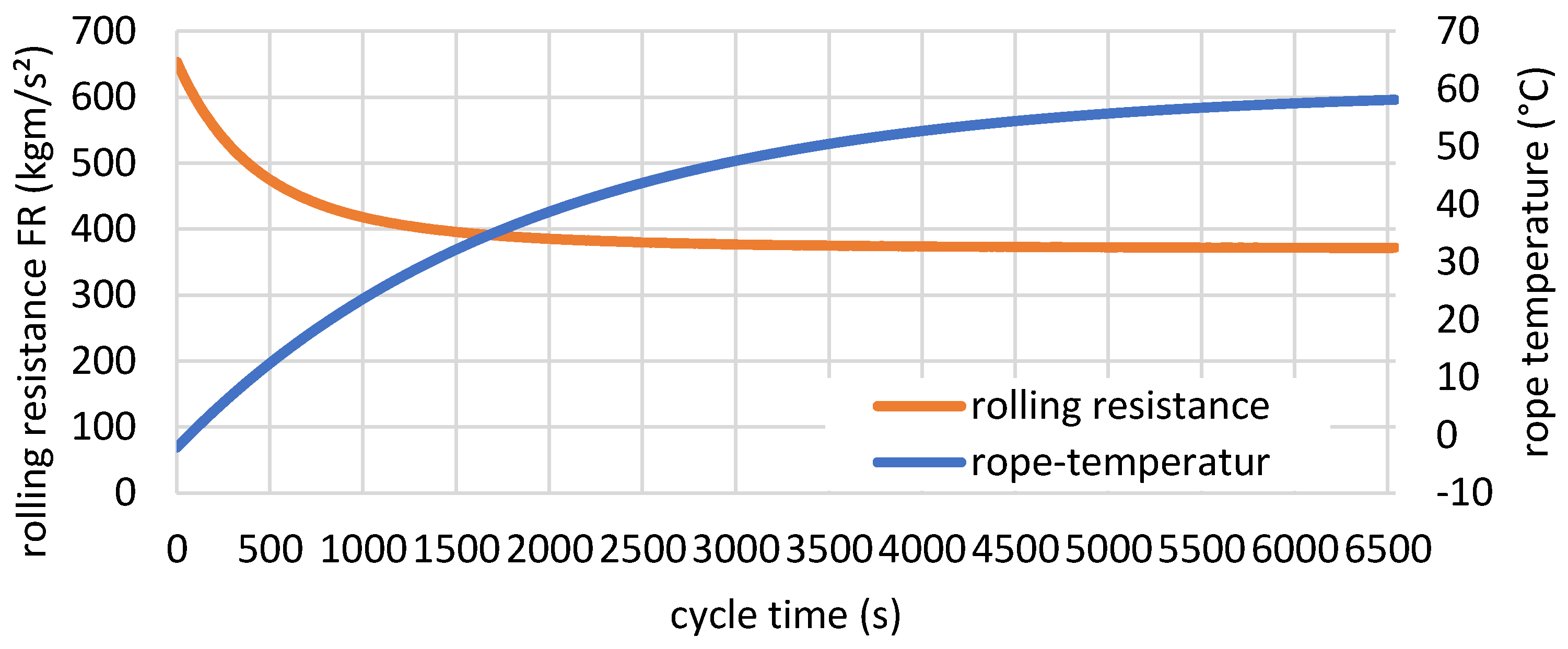
where $C_{\mathrm{r}}^{\mathrm{cold}}$ and $C_{\mathrm{r}}^{\mathrm{warm}}$ respectively denote the rolling resistance coefficient for the cold and the fully warmed-up tire, $T$ is the instantaneous temperature, and $T_{\mathrm{r}}$ is the reference temperature for $C_{\mathrm{r}}^{\mathrm{warm}}$. The consequences observed during a trip are described in more detail in Appendix C.1. The temperature of the cold tire is determined individually for each drive simulation depending on the season and the start time of the journey. Driving tests with relevant vehicles revealed that a value of 60 °C for $T_{\mathrm{r}}$ describes the conditions well [26].

Figure 2 shows a typical example of the resulting change of the rolling resistance force $F_{\mathrm{r}}$ during a trip. This change clearly cannot be neglected.

3.1.3. Gravity

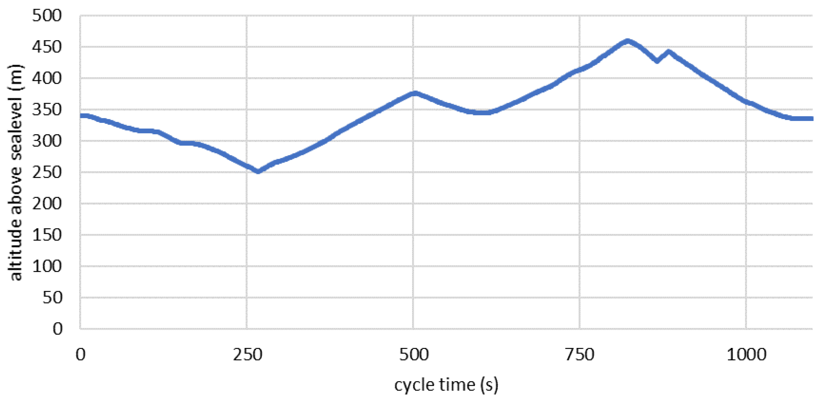
The gravity influence on the energy consumption during a trip results from elevation changes according to the known gravitational formula.

$$F_R=m·g·\sin \alpha$$

(5)

To generate generic data, we do not specify landscape shapes, but random elevation profiles with an average gradient of 3% for a hilly terrain (see Figure 3 for a typical example).

3.1.4. Mass Inertia

The force caused by mass inertia depends on the vehicle mass and on the acceleration:

$$F_a=m·a=m\frac{\mathrm{d}v}{\mathrm{d}t}$$

(6)

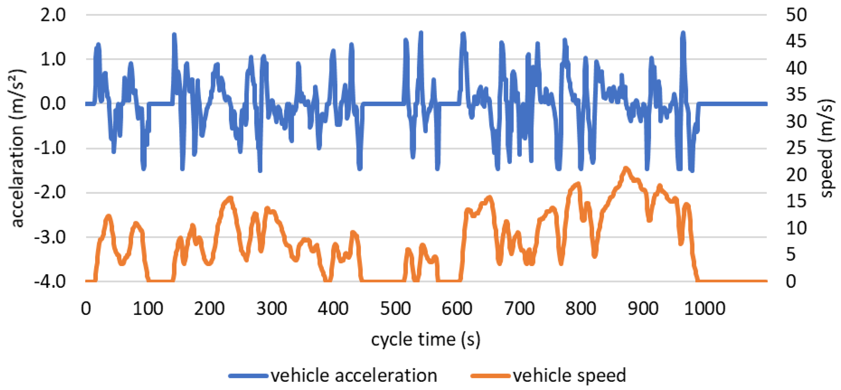
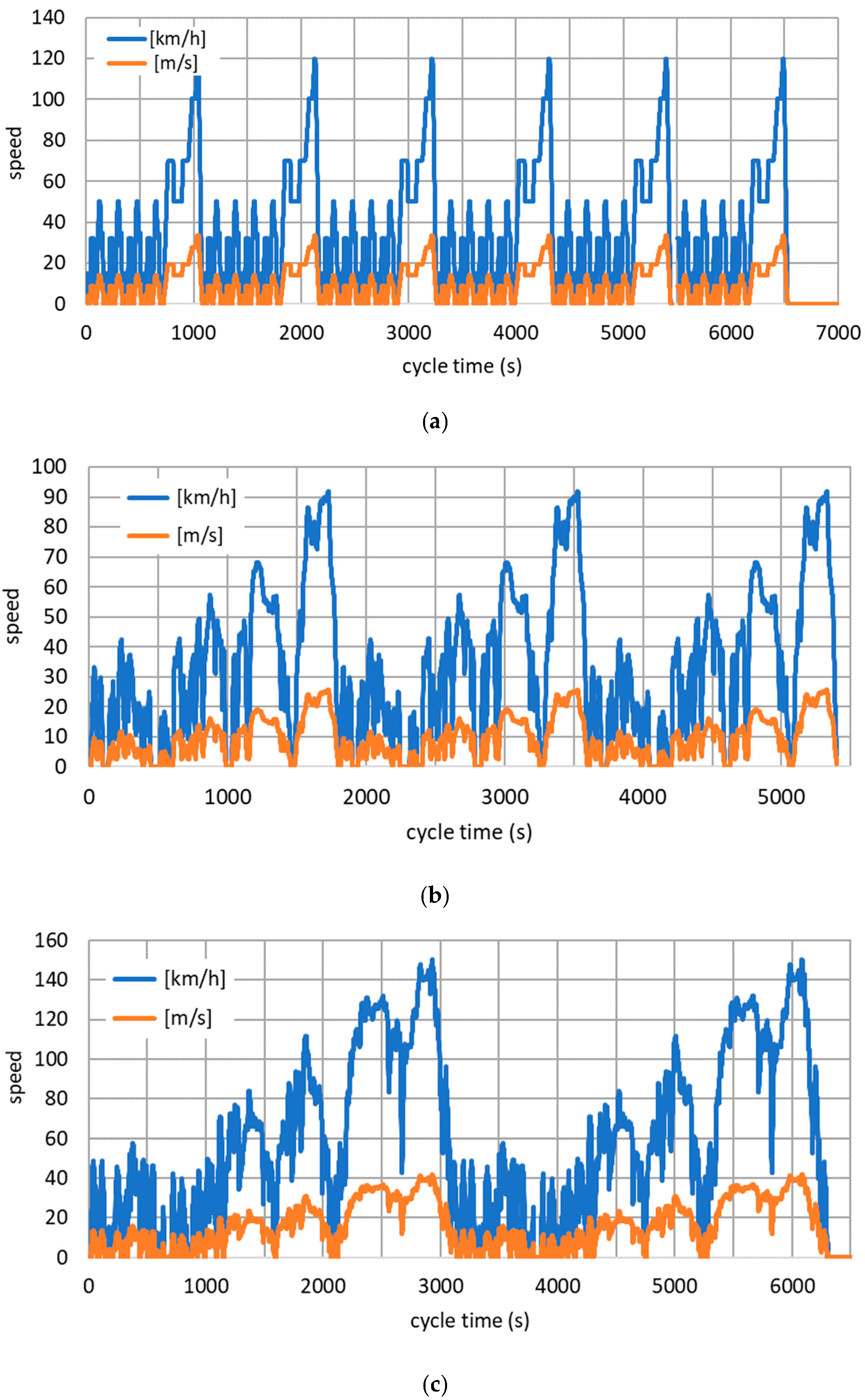
As described in Appendix E, the simulations were carried out by use of generic drive cycles (

Table A5. Composition of generic driving cycles.

Driving Pattern	Description	Duration/s	Length/km	Maximum Speed/(km/h)	Maximum Acceleration/(m/s2)
Passive	6 × NEDC	6540	64.9	119.8	0.92
Subcycle 1	NEDC	1090	10.8	119.8	0.92
Subcycle 2	— “ —	— “ —	— “ —	— “ —	— “ —
Subcycle 3	— “ —	— “ —	— “ —	— “ —	— “ —
Subcycle 4	— “ —	— “ —	— “ —	— “ —	— “ —
Subcycle 5	— “ —	— “ —	— “ —	— “ —	— “ —
Subcycle 6	— “ —	— “ —	— “ —	— “ —	— “ —
Standard	3 × WLTP	5400	50	91.9	1.23
Subcycle 1	Low–medium	1022	5.9	57.5	1.21
Subcycle 2	High–extra-high	778	10.8	91.9	1.23
Subcycle 3	Low–medium	1022	5.9	57.5	1.21
Subcycle 4	High–extra-high	778	10.8	91.9	1.23
Subcycle 5	Low–medium	1022	5.9	57.5	1.21
Subcycle 6	High–extra-high	778	10.8	91.9	1.23
Aggressive	2 × Artemis mix	6310	103.4	150.4	2.86
Subcycle 1	Urban	990	4.9	57.7	2.86
Subcycle 2	Rural	1090	17.3	111.5	2.36
Subcycle 3	Motorway 150	1075	29.6	150.4	1.92
Subcycle 4	Urban	990	4.9	57.7	2.86
Subcycle 5	Rural	1090	17.3	111.5	2.36
Subcycle 6	Motorway 150	1075	29.6	150.4	1.92

). These drive cycles stipulate the vehicle velocity as a function of time. This also determines the vehicle acceleration—see Figure 4, for an example—and, consequently, the inertial force.

3.2. Power Train and Transmission

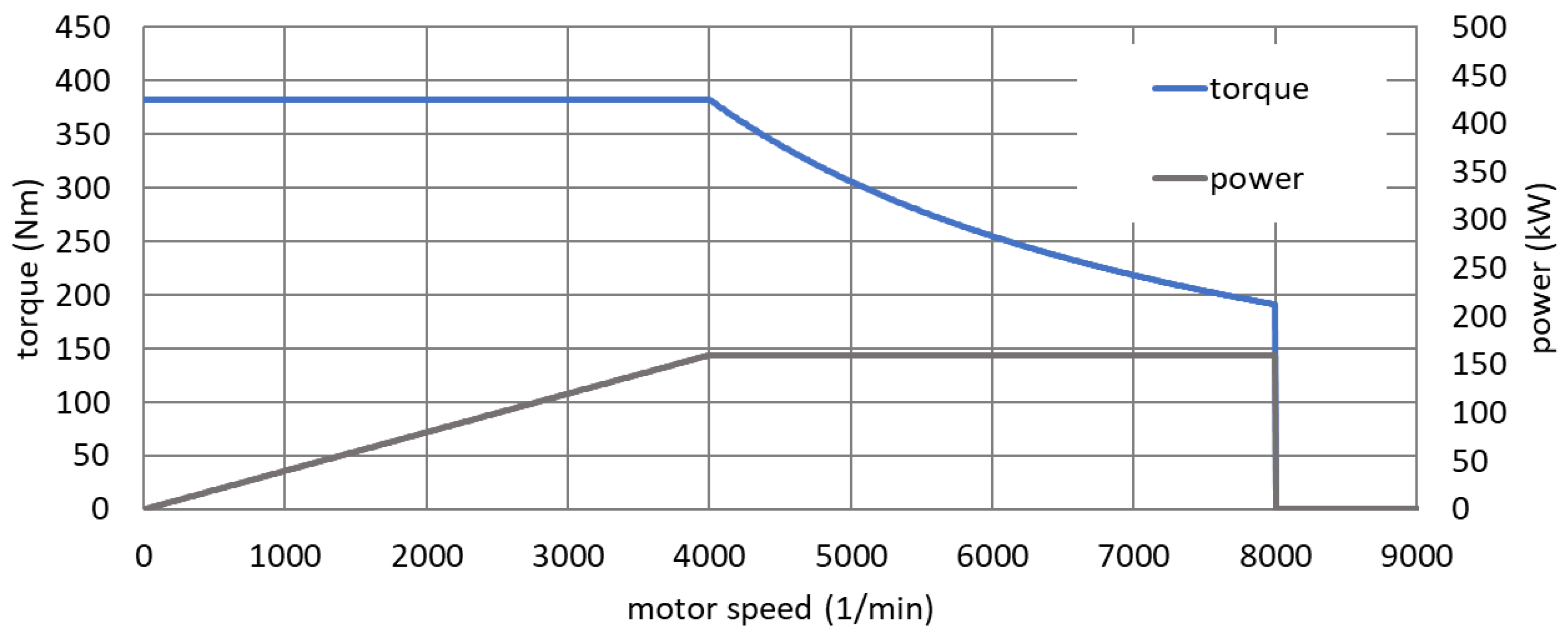
The powertrain of a BEV has a simpler structure than that of an ICEV. Not only the motor, but also the gearboxes usually contain fewer components and are less complex in design. This is because the electric motor develops constant and full torque, starting from zero speed. The full torque is available up to the so-called corner speed. Above this threshold, in the field-weakening range, the motor torque decreases with $1/n$ ($n$ = motor speed; see Figure 5) [27]. 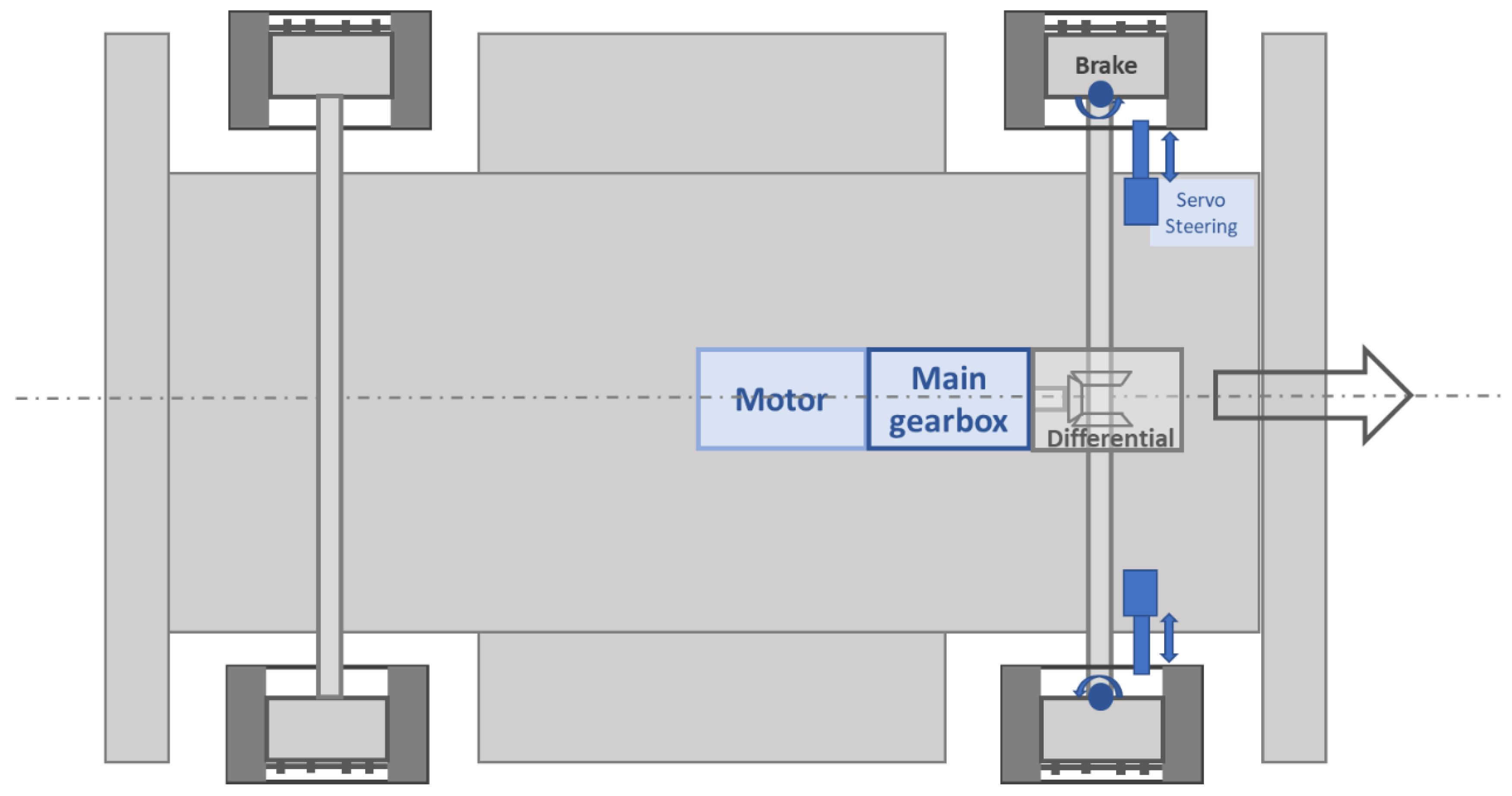In the field-weakening range, the turning rotor with its permanent magnets—a permanent-magnet (PM) motor is assumed for reasons explained in Section 3.3—induces a voltage that counteracts the primary field of the stator and can no longer be fully compensated by the voltage supply of the frequency inverter. The torque acting on the rotor decreases with the speed. The almost ideal control condition up to the corner speed and the wide speed range of the field weakening enable a conceivably simple transmission design. Similar to what is realized in practice in most BEVs, we have chosen a two-component system with one reduction stage each for the simulation (Figure 6).

The differential gearbox consists of a double bevel gear stage, which, on the one hand, compensates for the slightly different speeds of the left and right drive wheels. On the other hand, it diverts the power flow by 90° from the engine/main gearbox axle, which is in the direction of travel, to the transverse drive wheel axle with high efficiency. The power flow is divided in the differential gearbox according to the respective traction requirements of the two driven wheels.

The main gearbox, located between the electric motor and the differential gear, is usually directly adapted to the motor output shaft and consists of a highly efficient helical gear or planetary gear stage. For the purposes of our simulation, the main gearbox was assumed to have a helical gear stage with a reduction ratio of $i_{\mathrm{MG}}=2.5$ (small car) or $i_{\mathrm{MG}}=3.0$(small truck). In the main gearbox, the speed is reduced by the factor $i_{\mathrm{MG}}$, and the torque is increased by the same factor. An efficiency of 95% was assumed for the main gearbox. In the differential gear, we used a reduction of $i_{\mathrm{DG}}=2.0$ for both vehicle types with an efficiency of 92%. Adding the wheel bearings, to which we attributed an efficiency of 98%, results in a transmission efficiency of 85.7% for the entire driveline, calculated from the engine output shaft to the wheels.

3.3. Electric Motor

The key element of the power train is the electric motor. The torque/speed characteristics were already described in Section 3.2. A PM motor with rare-earth magnets is assumed because it is characterized by high magnetization, very low temperature dependence, excellent controllability, and, most important, high efficiencies of up to 90% for small machines and up to 95% for larger ones. The motor efficiency is significant in view of the valuable and limited battery storage capacity. Although an induction machine would be less expensive to manufacture, its lower efficiency of 75–85% would result in higher operating and lifecycle costs compared to the PM motor [28].

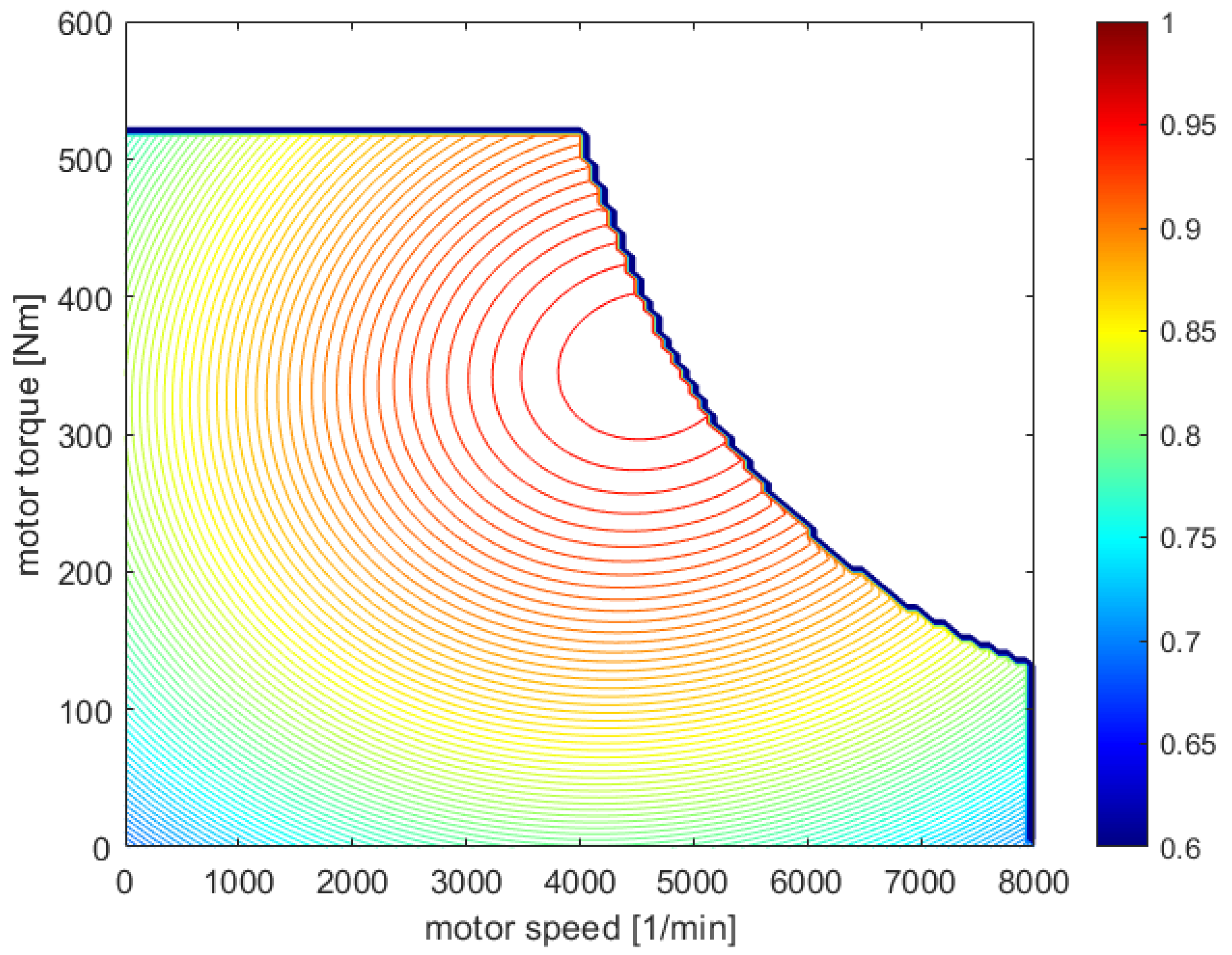
The basic efficiency behavior of the PM machine is well-known [29,30,31]. It depends on a multitude of design features of the motor: number of pole pairs, air gap size, slot filling factors, laminated stack design, arrangement of magnets, and many more. As already mentioned, we do not aim at statements about individual vehicles, but about vehicle classes, large fleets, technological influences, and societal impacts. Then it is not necessary to model the detailed characteristics of a particular motor. It rather suffices to describe the typical state-of-the-art at a given time. We used a mathematical model for the efficiency field of a generic PM machine which takes these requirements into account and can be applied to motors of different power classes (Figure 7). The model engine allows high speeds at limited torque (as in passenger vehicles) and lower speeds at high torque (as in trucks). Each combination of speed and torque is assigned a unique efficiency value.

The temperature dependence of the PM machine was neglected, because, in contrast to the induction machine, it has only a minor effect. A full thermodynamic model of the PM machine would have to include stator slot cross-sections, wire diameters, winding head dimensions, slot filling factors, and many more, thus leading to a design-dependent and complex description with little additional benefit. The parameters of the motor model are listed in Table A2 of Appendix B.

3.4. Inverter

The voltage supply and the speed control of the motor are provided by the inverter. Switching and non-harmonic losses, which account for the majority of the total inverter losses, have become quite small in recent years. By use of silicon carbide technology efficiencies of up to 99% are announced for future generations of inverter [32,33]. For the purpose of the present simulations, a constant inverter efficiency of 96% was assumed as described in the related literature [34].

3.5. Battery

The further development of battery technology is crucial for the speed of the spread of electrical mobility. To achieve acceptable ranges with BEVs, an energy storage capacity of about 100 kWh is required in passenger vehicles and up to 1500 kWh in commercial vehicles. If at all, only the most powerful lithium-ion batteries are capable of this. We assume the state-of-the-art given by a LiFePO₄ battery in our model (

Table 4. Technical data of a LiFePO₄ battery [36].

Item	Value
Number of cycles (90% DoD)	5000
Life cycle range/km	1.5 × 106
Energy density by mass/(Wh/kg)	200
Energy density by volume/(Wh/L)	500
Efficiency of discharge/%	95
Efficiency of charge/%	95
Lower SoC limit/%	5
Upper SoC limit/%	95

). It uses graphite as the cathode material and LiFePO₄ as the anode material and offers several important advantages. The anode no longer contains the metals cobalt, nickel, or manganese, the mining of which is ecologically and socially problematic. In addition, the short-circuit resistance of this battery is higher than that of the lithium-ion batteries used to date. This reduces the risk of fires that are difficult to extinguish. Finally, LiFePO₄ batteries have high cycle stabilities and long lifetimes, and this favors recycling and secondary use. Tesla, the leading BEV manufacturer, has recently announced that it will also use LiFePO₄ batteries in its next generation of vehicles [35].

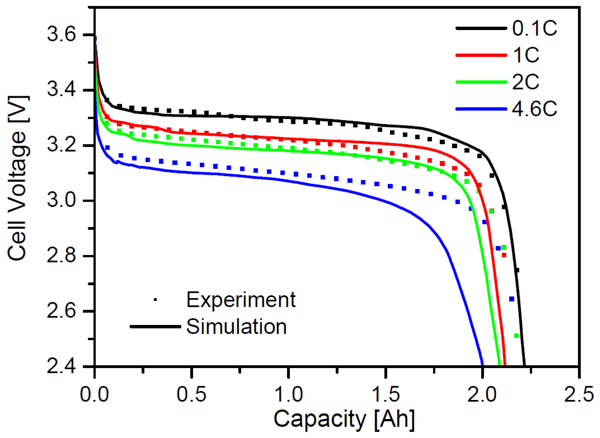
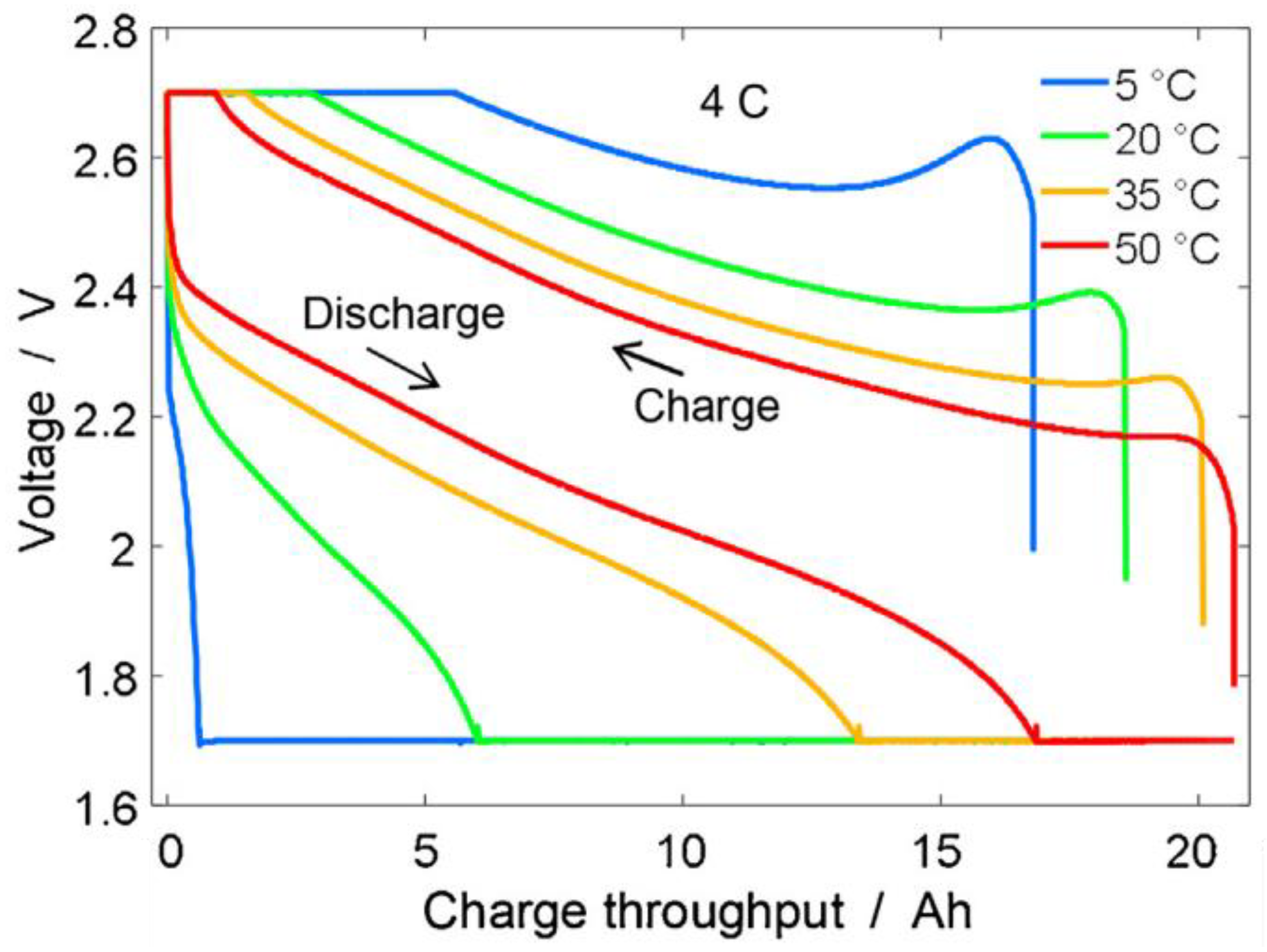
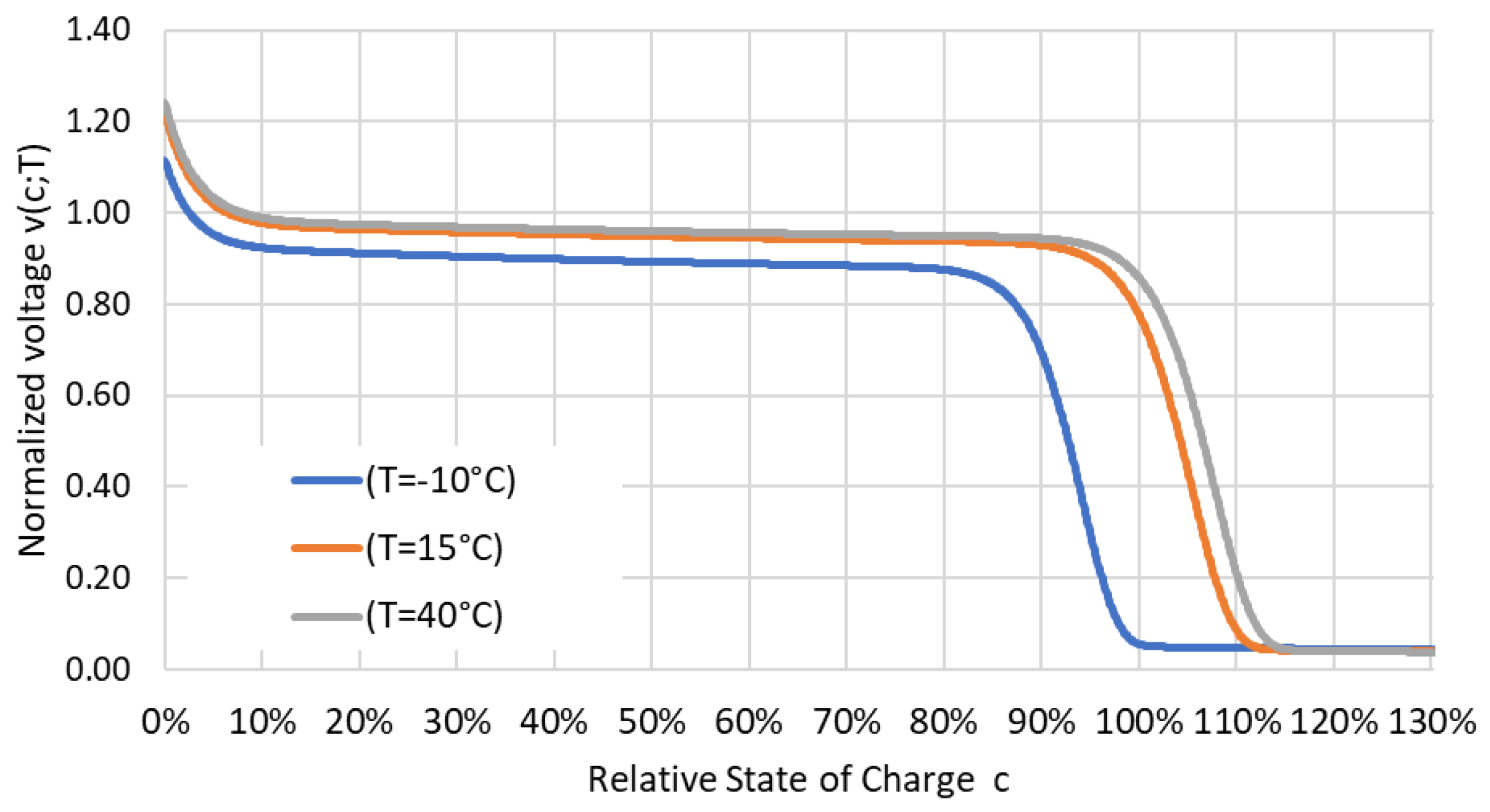
The battery performance depends on the temperature and the terminal current. The output power (e.g., in kW) is usually referred to the rated battery capacity (e.g., in kWh). This normalized power, or “C factor”, when expressed in 1/h, describes which part of the capacity can be charged or discharged in one hour. The discharge rate has a significant effect on the voltage and capacity of the battery for C > 1.5 (Figure 8). When dimensioning the vehicle components in our study, we ensured that C always stayed below 1.5.

It is known from practical experience that cold starts and cyclical braking/acceleration (e.g., in winter, with urban cycle) affect the efficiency, capacity, and lifetime of the battery in a negative way [38,39]. The temperature behavior of the battery, as shown in Figure 9, is well modeled by a functional approximation which is described in Appendix C.2, Figure A1.

The battery model used was confirmed by the good agreement of the determined battery efficiency values with the cited literature values. The simulations presented in Section 4 resulted in efficiency values between 93% and 96% and 94.2% on average. This value was calculated as the ratio of the electrical energy supplied to the inverter to the battery charge consumed at nominal voltage.

3.6. Recuperation

In contrast to the ICEV powertrain, an electric powertrain allows the recuperation of excess kinetic energy because the electric engine can be operated both as motor and as generator. The control program, which regulates the driving speed based on the driving profiles, always tries to prioritize recuperation before braking. In our simulations, recuperation factors between 65% and 69% were achieved.

The regenerative braking effect of the electric engine was large enough in all simulations, as presented in Section 4; below that, no kinetic energy had to be dissipated by the brakes. This surprising result is due to the use of well-defined driving profiles that do not include unplanned situations with full braking.

3.7. Vehicle Accessories

The simulation model considers the following vehicle accessories: air conditioner, instruments, seat-heating, lighting, and servo-steering. The nominal consumption values of these components were taken from the technical literature [40,41]. Depending on time of day, season, and geographic location, the ambient temperature and the lighting conditions are determined, and the consumption data of the vehicle accessories are derived from them.

Table A4. Model parameters for a trip with a small truck in Northern Bavaria, Germany, in January. A generic driving cycle with passive driver behavior was assumed (repeated NEDC with a duration of 6540 s or 1.82 h; see Table A5).

Item	Value
Trip details
Average temperature during drive cycle/°C	−1.29
Daylight time	8:00 a.m. to 16:30 p.m.
Start time	7:00 a.m.
Duration of trip/h	1.82
Travel time by day/h	0.82
Travel time by night/h	1.00
Air conditioning
Rated power/kW	0.9 [41]
Scaling factor at 20 °C … 35 °C/%	25 … 100
Scaling factor valid for trip/%	25
Total energy consumption on trip/kWh	0.409
Seat heating
Rated power/kW	0.25
Scaling factor at 0 °C … 25 °C/%	100 … 0
Scaling factor valid for trip/%	100
Total energy consumption on trip/kWh	0.454
Instruments
Rated power/kW	0.15
Scaling factor by day and by night/%	50/100
Scaling factor valid for trip/%	77.52
Total energy consumption on trip/kWh	0.211
Lighting
Rated power/kW	0.30
Scaling factor by day and by night/%	50/100
Scaling factor valid for trip/%	77.52
Total energy consumption on trip/kWh	0.423
Servo steering
Rated power/kW	0.75 [40]
Total energy consumption on trip/kWh	1.363
All accessories together
Total energy consumption on trip/kWh	2.859

in Appendix D provides a calculation example.

4. Results

4.1. Scenario Description

In Section 1, the literature and own tests were shown to provide evidence of significant differences between the actual maximum range of a BEV and the manufacturer specifications. The results obtained with our simulation platform and about to be presented in this section serve to shed light on the details of BEV energy consumption in the real world (rather than on test benches).

Table 5. Scenario parameters for BEV range and consumption simulations.

Item	Values Used in Current Simulations
Vehicle class	Small car | small truck
Drive system	Electric motor (PM)
Energy storage	LiFePO4 battery
Technology status	2020
Driver attitude	Passive (NEDC) | standard (WLTP) | aggressive (Artemis)
Season	Summer | spring/autumn| winter
Terrain	Flat | hilly

lists the scenario parameters used for the simulations of this work. The drive type chosen was always the electric motor described in Section 3.3 within the drive train described in Section 3.2. Likewise, the battery described in Section 3.5 was used as the energy storage device in all simulation runs. The performance characteristics of the selected drive elements correspond to the current state-of-the-art (2020). The rapid development advances in battery technology, semiconductor, and magnet technology will likely lead to better performance in the future. The potential effects of assumed advances can then be studied by varying the performance characteristics in the simulation.

In this work, we present the results of investigations involving all combinations of two vehicle classes, three driver attitudes, three seasons, and two terrain characteristics (36 combinations in total; see Table 5).

The reason for including not only passenger vehicles but also commercial vehicles is that the latter are responsible for a large proportion of pollutant emissions [42]. If one wants to make statements about the entire transport sector, they cannot be ignored. The characteristics of the two vehicle classes are listed in Table A2 of Appendix B. Furthermore, it is known from the literature that the individual behavior of the driver has a considerable influence on the consumption and range of a BEV [22,43]. We therefore looked for ways to include different, yet standardized and reproducible driving behaviors. In the end, we defined three types of drivers: passive, standard, and aggressive. Each driver type is assigned a generic driving cycle, as described in Appendix E. The cycles model 1.5-to-2-h trips with representative mixes of urban, rural, and motorway driving.

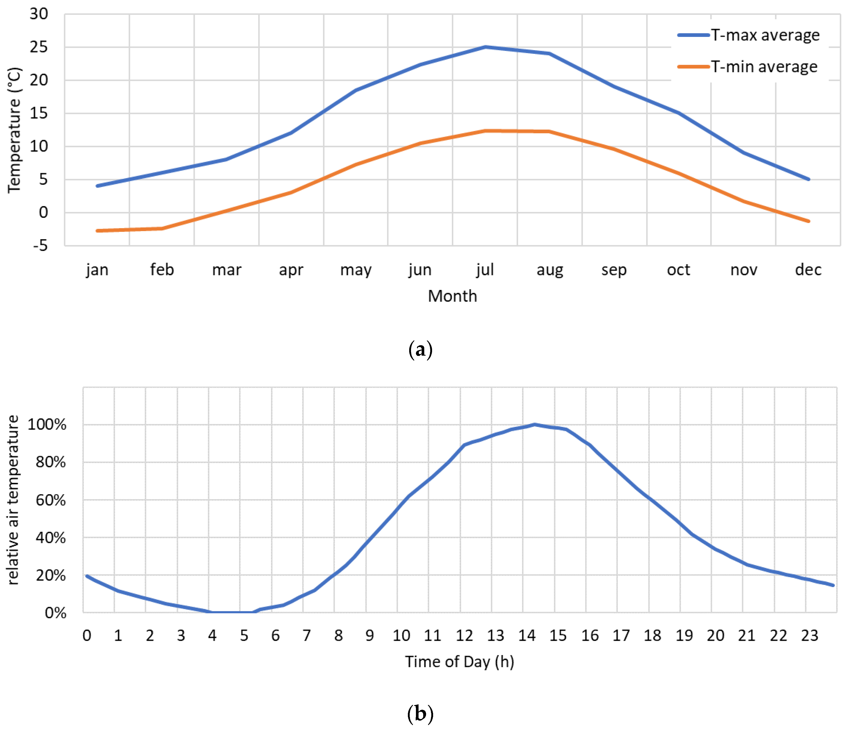
In order to account for the temperature influence, the BEV subsystems that show an appreciable temperature dependence are represented by suitable temperature models, as described in Section 3.1.2 and Section 3.5 and Appendix C. Furthermore, the seasonal and intraday temperature variations typical of Germany were taken into account (see Appendix C.3, Figure A2). This and the duration of daylight distinguish the different seasons.

As already mentioned, the influence of the terrain character on consumption and range is appreciable [44,45]. This is especially true for vehicles with large battery capacity and correspondingly heavy mass. For the purpose of our studies, we did not use real landscape profiles, but randomly generated artificial elevation profiles with a preset mean inclination of 3%. All profiles would be selected such that the starting and ending points had the same elevation. Thus, the net overall height difference was zero for each simulation and all selected profiles.

4.2. Range of Small Passenger BEVs and Small BEV Trucks

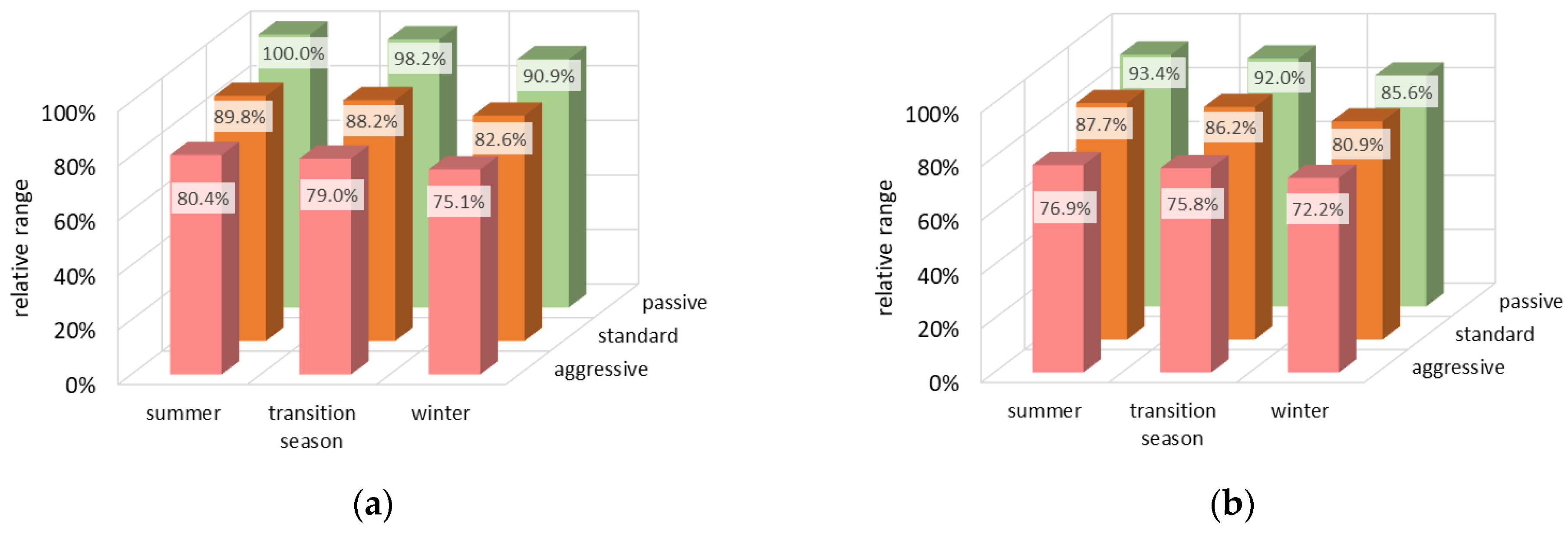
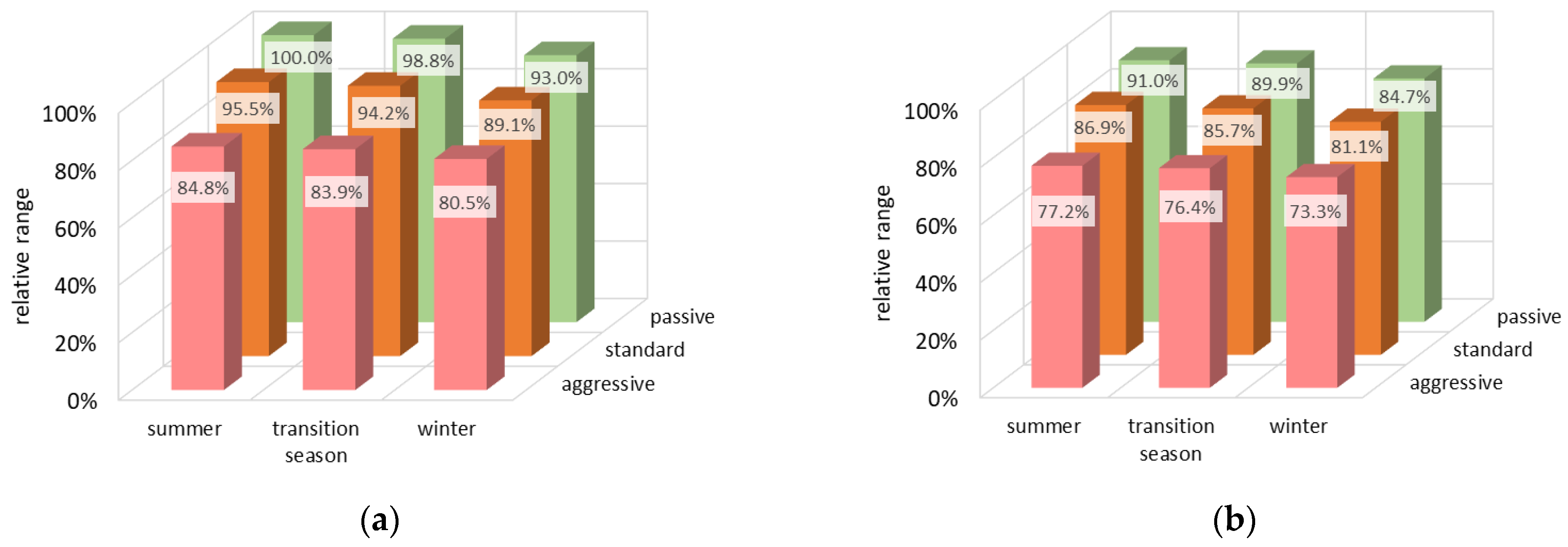
The scenario leading to the greatest range is a summer trip on flat terrain with a passive driving attitude, both for passenger and commercial vehicles (see

Table 6. BEV consumption and range values (passive driving behavior, summer season, flat terrain).

Vehicle Class	Specific Consumption/kWh/(100 km)	Effective Battery Capacity/kWh	Range/km
Small car	16.6	54	326
Small truck	$42.3$	108	255

for numbers). All other scenarios were referred to the respective best case for each of the two vehicle classes considered. This representation offers the advantage that it is independent of the battery capacity of the vehicle. Figure 10 (for passenger BEVs) and Figure 11 (for BEV trucks) show the relative numbers in dependence of the season, the driving behavior, and the terrain type. The numerical cruising-range difference between best-case and worst-case scenarios of roughly 30% reminds one of the numbers discussed in Section 1.

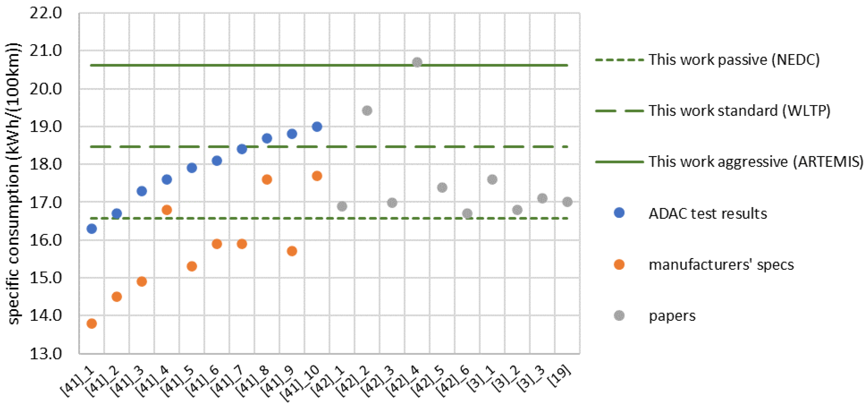
We repeat that these results were obtained with preset parameter values and that no parameter was varied to improve the agreement between model prediction and independent observations. It is all the more impressive how well the simulations agree with independent data from the literature [3,21] and real consumption measurements [46]. This agreement, visualized in Figure 12, serves as validation of the model. As of now, a large number of independent data are available for state-of-the-art passenger BEVs, but it must be noted that no sufficient database for trucks exists. We believe that our results can contribute to close this data gap.

One strength of our approach is that it allows us to quantify the various real-world influences on energy consumption. Figure 10 and Figure 11 lead to the following statements:

• Winter conditions reduce the BEV range by 8% (small car) and 9% (small truck), respectively.
• A hilly terrain reduces the BEV range by 7% and 9%, respectively.
• The strongest influence on consumption and range comes from the individual driving behavior. An aggressive driving style reduces the BEV range by 20% (small car) and 17% (small truck), respectively.

Addition to Figure 12: ADAC is the General German Automobile Club, Europe’s largest motoring association.

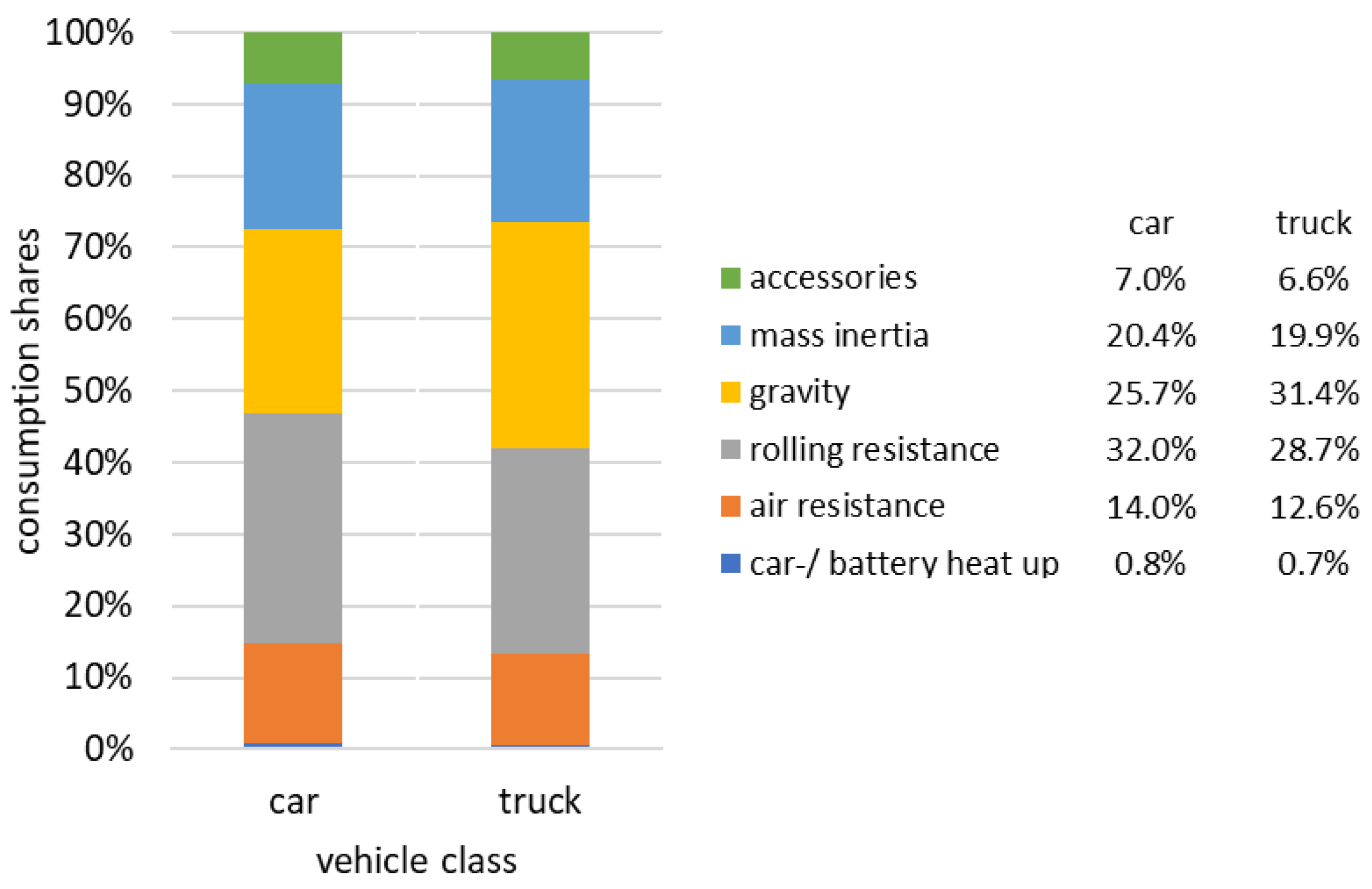
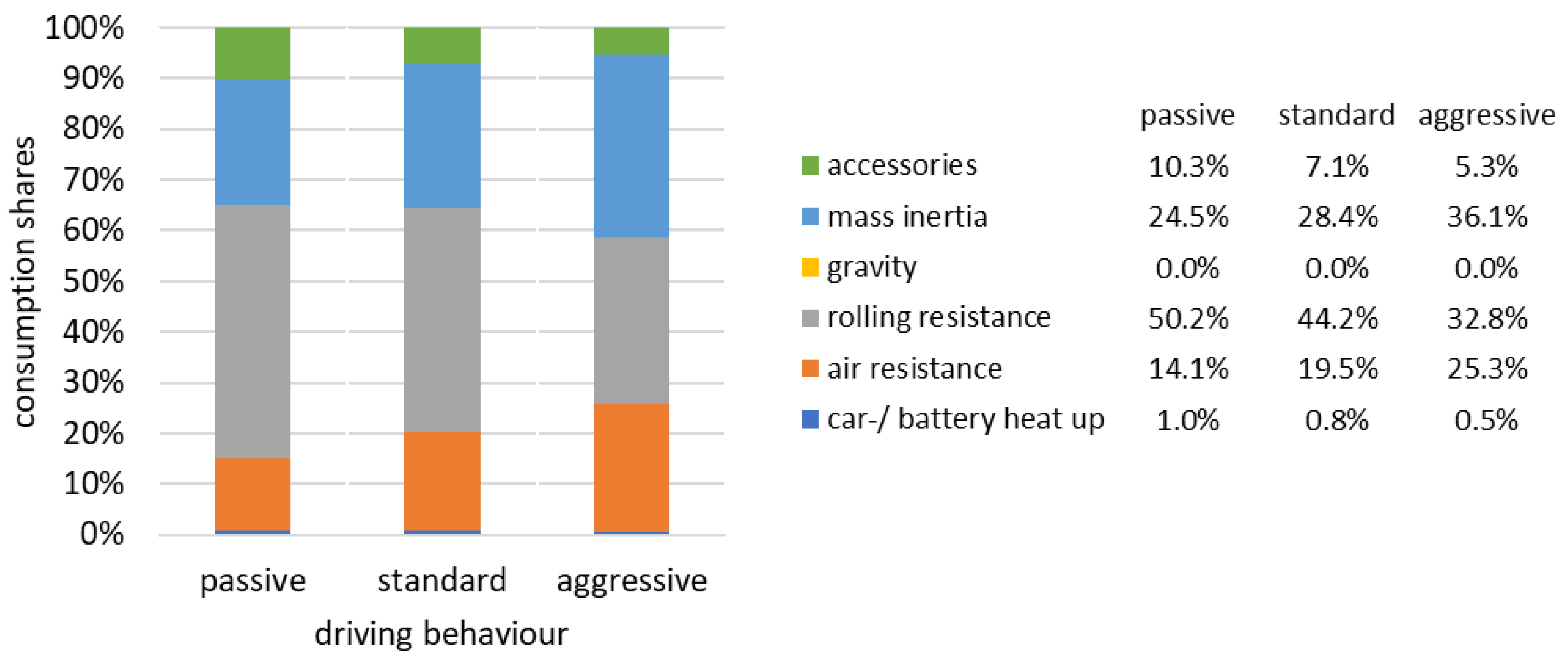
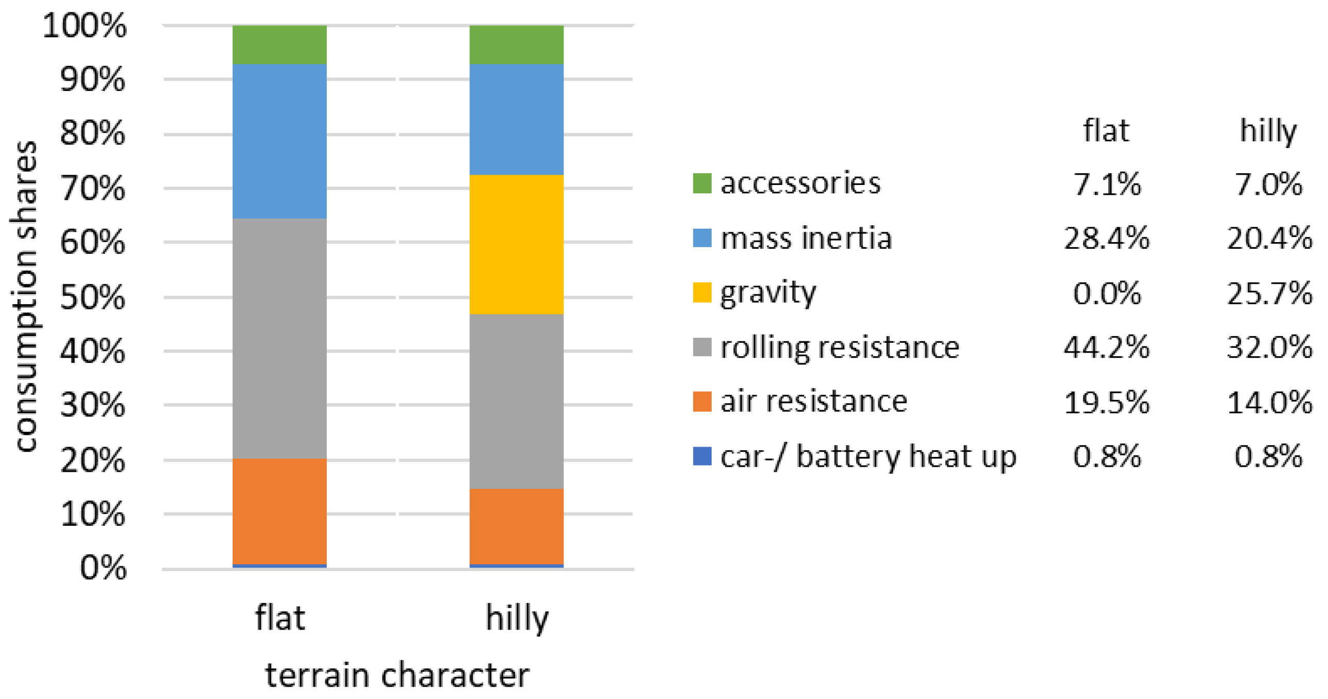
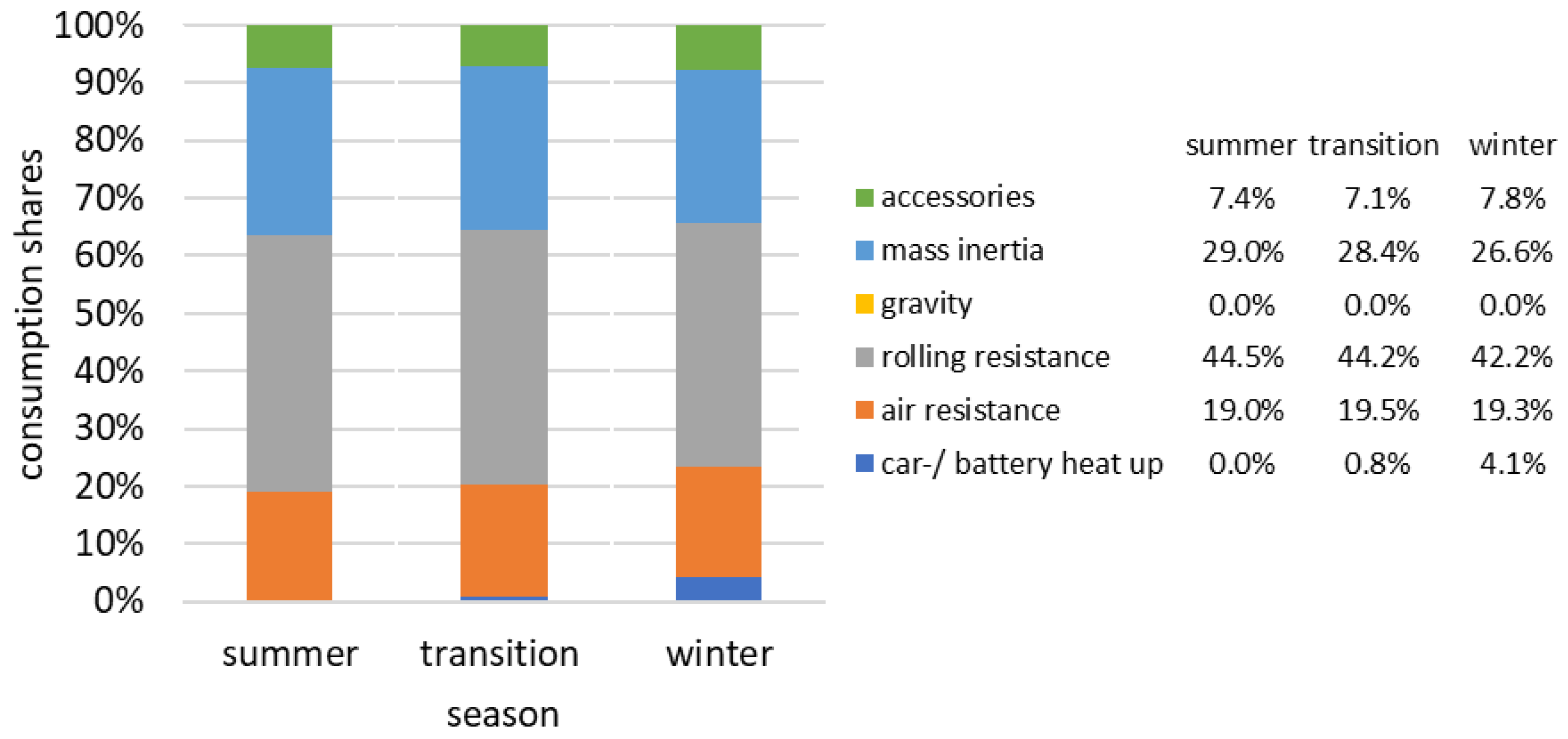
4.3. Consumption Shares in Small Passenger BEVs and Small BEV Trucks

A further use of our simulation platform, which cannot be substituted by practical tests, is to make detailed statements about the consumption shares in BEVs. Only in this way will it be possible to further develop the entire BEV powertrain in a targeted manner. The results provide information about the main consumption shares caused by various physical forces and about peripheral consumers, such as accessories and preheating. Preheating of the battery is a BEV-specific concept intended to bring the battery into the optimum operating temperature range during the cold season, with the aim of minimizing overall power consumption and optimizing battery life. Further research will be required on this detailed topic in order to be able to make accurate statements about the effectiveness of preheating in terms of consumption and service life.

Figure 13, Figure 14, Figure 15 and Figure 16 summarize our findings about the consumption shares. Each figure presents the influence of the mentioned variable parameter by keeping the other parameters constant.

Unlike an ICEV, the BEV can convert kinetic energy back into battery charge via the regenerative effect of the electric motor. This recuperation leads to a significant reduction in energy consumption, as shown in

Table 7. Reduction of BEV consumption by recuperation (small passenger BEV, standard driving behavior, transition season, and hilly terrain).

Item	Value
Recuperation factor/%	64.9
Recuperated energy/kWh	−2.37
Total energy consumption/kWh	13.99
Theoretical energy consumption without recuperation/kWh	16.36

by way of an example. In this example, the saving due to recuperation is approximately 15% in relation to the theoretically extrapolated consumption without recuperation. Recuperation only results from kinetic energy or from potential energy in the gravitational field of the earth. In acceleration-free driving without altitude differences, there can be no recuperation. When looking at the consumption shares, it is therefore physically correct to credit the recuperated energy to the inertial mass and gravitational components in proportion to their accumulated force components. We followed this line of reasoning for Figure 13, Figure 14, Figure 15 and Figure 16 and for

Table 8. BEV consumption shares with and without recuperation.

Quantity	Consumption Share/%
	With Recuperation	Without Recuperation
Car/battery heat-up	0.8	0.7
Air resistance	14.0	8.5
Rolling resistance	32.0	19.6
Gravitation	25.7	29.8
Mass inertia	20.4	35.5
Accessories	7.0	6.0

.

Table 8 clearly shows that recuperation reduces the relative consumption shares of inertial mass and gravity. As a result, the other consumption shares from air resistance and rolling friction are much more significant than for combustion vehicles. This finding must direct the focus of BEV development besides vehicle weight also on reducing rolling and air resistance. On the other hand, it can be seen that aggressive driving or driving in a hilly environment has a less serious effect on consumption.

Altogether, based on Figure 10 and Figure 11, we make the following statements on consumption shares:

• For BEV trucks, the single most important contributor to energy consumption is gravity with a share of about 30%. This is a consequence of the weight of the payload and means that accurate range predictions for commercial vehicles are only possible with knowledge of the specific altitude profile.
• Increasing safety requirements and growing comfort desires cause non-negligible consumption in the accessories of BEVs (power steering, air-conditioning, communication, display, etc.). This reduces the cruising range by 7%, which is completely in line with field data [41].
• Preheating the battery accounts for 4% of consumption in winter. Further studies must show to what extent this consumption share can be reduced with new battery technologies and improved control strategies.
• Recuperation converts about 65% of the available kinetic energy into battery charge. This reduces BEV consumption by about 15%. Recuperation reduces the additional consumption caused by aggressive driving or driving in hilly terrain.

5. Conclusions and Outlook

Our studies have shown that, despite the complexity of BEV consumption data determination, a remarkable agreement with empirical data is possible with a model that only works with parameter values known a priori and that can be implemented with common desktop computer software. We were able to provide further evidence as to why manufacturer specifications systematically and significantly deviate from real-world consumption values (see Section 4). One reason for the model success may be that the action of an electric powertrain can be described more easily by physical models than is the case with internal combustion engines. The range of our results is in agreement with more than 90% of the relevant literature values or practical test results (see Figure 12).

Only a rather incomplete database exists for electrically driven commercial vehicles. It has been shown that the BEV passenger vehicle models, confirmed by a sound database, can be transferred very well to commercial vehicles. Despite the strong dependence on the payload and the altitude profile during a trip, a convincing agreement with the available literature values has been achieved ([47], Table 1; [48], Table 6). This opens the door for future studies on commercial vehicles to create a reliable database for assessments of consumption and greenhouse gas emissions.

In contrast to practical tests, the physical simulation model allows statements to be made about consumption shares that can be assigned to various physical origins. This, in turn, allows important findings to be derived for the further development of BEVs. Simple parameter variations can be used to make predictions about future vehicle variants.

The recuperation of kinetic energy in the electric powertrain significantly changes the consumption structure well-known from the ICEV. This allows us to increase the range of BEVs by about 15%. The simulation results show that additional influencing variables must be considered for the development of future BEVs. For example, rolling resistance must be given greater consideration again.

Finally, with the help of the available individual simulation results, the consumption and emission data of entire vehicle fleets can be predicted sufficiently well. Important findings can be derived for essential areas of energy research on the basis of the results presented. The sector of renewable energy generation and distribution is significantly influenced by the transformation of the mobility sector. If only the manufacturers’ data on vehicle consumption were used for energy provision, a serious supply gap of almost 30% would result—with very bad consequences for the entire economy.

Other sectors within future mobility, such as charging technology, charging infrastructure, energy storage with decentralized battery networks, and power2gas-generation-issues, can benefit significantly from the specification of the actual consumption values of BEVs. Important statements can thus also be made for the mobility/electricity sector coupling and the supply of raw materials in the production of the necessary vehicle components.

The present study represents an important milestone for us on the further path of this development. In future projects, we want to broaden the perspective from the previously considered vehicle types passenger cars and light commercial vehicles to include also heavy commercial vehicles, as their contribution to GHG emissions is significant. In order to do this, it will be necessary to expand the technology horizon because of the large range requirements of heavy trucks. Not only the combination of electric motor and battery should be considered. The use of hydrogen-based fuel cell drives and combustion drives that work with renewable methane will also be analyzed and compared with the BEV. While so far only consumption and range have been determined in this study, in the future the GHG emissions of the different drive types will also be considered. As a matter of fact, the GHG emissions are the essential parameter in the Kyoto and Paris Protocols, which the target reductions until 2050 are derived from. This is intended to make a further contribution to better assessing the extent to which the goals set there will be realistic.