Evaluating the Combined Effect of Climate Change and Urban Microclimate on Buildings’ Heating and Cooling Energy Demand in a Mediterranean City

Abstract

Climate change has a major impact on the urban built environment, both with respect to the heating and cooling energy requirements, but also regarding the higher probability of confronting extreme events such as heatwaves. In parallel, the ongoing urbanization, the urban microclimate and the formation of the urban heat island effect, compounding the ongoing climate change, is also a considerable determinant of the building’s energy behavior and the outdoor thermal environment. To evaluate the magnitude of the complex phenomenon, the current research investigates the effect of climate change and urban heat island on heating and cooling energy needs of an urban building unit in Thessaloniki, Greece. The study comparatively evaluates different tools for the generation of future weather datasets, considering both statistical and dynamical downscaling methods, with the latter involving the use of a regional climate model. Based on the output of the regional climate model, another future weather dataset is created, considering not only the general climatic conditions, but also the microclimatic parameters of the examined case study area, under the future climate projections. The generated future weather datasets are then used as an input parameter in the dynamic energy performance simulations with EnergyPlus. For all examined weather datasets, the simulation results show a decrease of the heating energy use, an effect that is strongly counterbalanced by the rise of the cooling energy demand. The obtained simulation results also reveal the contribution of the urban warming of the ongoing climate change, demonstrating the need to perform a holistic analysis for the buildings’ energy needs under future climate conditions.

1. Introduction

Climate change refers to continuous changes in the distribution of weather patterns that range from decades to millions of years [1]. The Mediterranean region is highly susceptible to changes in climate and will be severely affected, as it will become warmer and drier with an increased frequency of extreme weather events, such as heat waves and extreme precipitations [2,3]. It has been also characterized as a “hot spot” by the scientific community, as the future warming and the decrease in precipitation are expected to be more pronounced in this area in contrast to the global mean change [4,5].

According to the IPCC Fifth Assessment Report [6], the climate system is affected by human activities and anthropogenic GHG emissions, the atmospheric concentration of which have increased significantly during the last years due to the economic growth, the use of natural sources of energy (non-renewable) and population growth. The effects of these concentrations in the climate system, combined with those of other anthropogenic factors (e.g., land-use change), may be the main cause for the observed rise in temperature since the mid-20th century. The observed climate changes have severely affected the human and natural environment. The temperature of the atmosphere and the oceans has increased, the amount of snow and ice has decreased, and the sea level has risen. The global mean surface warming, until the end of the 21st century, has been determined mainly by the cumulative CO₂ emissions. The continuous emission of GHGs will lead to further warming and long-term changes, causing more severe effects to humans and ecosystems.

In order to analyze the possible climate change and its impacts and to propose possible mitigation techniques, IPCC developed a series of different scenarios (Special Report on Emissions Scenarios—SRES) that represent the main driving forces of future emissions (economic, technological and population growth). There are four “families” of scenarios, A1, A2, B1 and B2, and within the A1 “family” there are three different groups (A1FI, A1T and A1B) according to the development of energy technologies [7]. In the Fifth Assessment Report, IPCC introduced the Representative Concentration Pathways (RCPs), an up-to-date package of emission scenarios, which are used in climate models for the future projections of climate. These pathways include concentration and emission scenarios of GHGs, as well as information for factors, such as stabilization and mitigation scenarios, land use and socioeconomic conditions. Four different RCPs have been developed and considered as representative of the literature [8]. They include a declining pathway that leads to very low radiative forcing (RCP2.6), two intermediate stabilization pathways (RCP4.5/RCP6) and a high radiative forcing pathway (RCP8.5). Future emission scenarios are the main input data for General Circulation Models (GCMs), the models that are used for the evaluation of the future climate change and provide climate data at spatial resolution of 150–300 km. Hence, to achieve a regional increase in resolution, the use of nested Regional Climate Models (RegCMs) is employed to account for sub-GCM grid-scale forcing. A detailed overview of downscaling techniques is provided in the following sections.

Diffenbaugh et al. (2007) [9] have used regional climate models to assess the heat stress intensification in the Mediterranean region under two SRES emission scenarios. The authors found that the occurrence of hot extremes, and as a result the intensification of heat stress risk, in the Mediterranean region increases dramatically (200–500%) due to the pronounced greenhouse gas concentrations. In the study of Zanis et al., 2015, [10] the use of forecasting regional climate models under the A1B SRES emission scenario for the Greek region led to an annual increase of temperature which was more intense at the end of the century. Tolika et al. (2012) [2] assessed the potential future changes in temperature for Greece with the use of various regional climate models under three SRES emission scenarios. The results of this study showed a rise in temperature over the area of study which is more intense during summer. Regarding future climate change in Greece [11], future projections with an up-to-date regional climate model under RCP4.5 emission scenario showed an increase of temperature by 2.0–3.0 °C until the mid of the 21st century, with a peak increase by 3.6 °C at the end of the 21st century. It is also worth mentioning that the peak intensity of temperature rise is expected to occur during summer months, while the highest rise of temperature is detected in the southern part of Greece (Figure 1).

Based on the existing scientific evidence, it becomes obvious that the climate change contributes to longer, more severe and more frequent heat waves. Particularly the urban areas, which already experience the negative consequences of the heat island effect, are expected to face extreme heat events. In fact, the increase of the air temperature in urban areas is further intensified by the thermal and optical (absorbent, non-reflective) properties of conventional building materials [12,13], the reduced evapotranspiration due to plant deficiency [14], the anthropogenic production of heat, as well as the atmospheric pollution [15].

Undoubtedly, the increased urbanization along with the ongoing climate change and the accompanying rising temperatures and extreme heat waves are considerable determinants of human thermal comfort and well-being on one hand, and of the building’s energy behavior on the other. More precisely, considering that the buildings’ heating and cooling energy needs are strongly related to their immediate microclimatic conditions [16,17], it becomes clear that a further increase of air temperature due to the climate change on the already degraded urban environment will significantly affect the energy demand especially in summer periods, which will in turn burden the urban environment with additional heat and pollutants’ emissions [18].

It becomes obvious that the selection of suitable weather data, accounting for the warming both from climate change and urban warming, is critical towards the acquisition of high accuracy energy performance simulation results on the one hand, and the suggestion of suitable mitigation and adaption strategies on the other. To date, current Building Energy Performance Simulation (BEPS) tools generally use typical weather files that are based on the statistical analysis of historical records at meteorological stations located in the peripheral zones of cities [19]. However, this practice does not allow for the consideration of the magnitude of climate change.

On the other hand, as previously mentioned, the evaluation of climate change and the climate forecasting is conducted using the General Circulation Models or Global Climate Models (GCMs) [20]; however, these models provide climate information on the global scale and with a large spatial and temporal resolution. Consequently, the direct use of their output on dynamic building energy performance simulation tools would not be possible, as the latter requires climatic parameters at an hourly resolution. In order to acquire compatible, future climate data, the GCMs should be downscaled, and to this aim, there are two main approaches involving dynamical and statistical downscaling methods (see Section 2).

At this point it must be emphasized that, in the existing literature, numerous studies have employed either statistical or dynamical downscaling approaches to assess the impact of climate change on the buildings’ energy performance [21,22,23,24,25,26]. Yet, in all these cases, the buildings’ energy performance is assessed only for the general governing climatic conditions without considering the microclimatic conditions characterizing each study area. As a result, the complex processes that occur between building blocks, solar radiation and wind speed, determining the urban climate are neglected. Nonetheless, given that the buildings’ energy demand is strongly correlated to the climatic conditions of the study area [16], it becomes obvious that the acquisition of high accuracy building energy simulation results necessitates a deep knowledge of the microclimatic conditions of each study area, as well as the consideration of future climate change.

In this context, the present paper aims to examine different methods for generating future weather datasets for dynamic building energy performance simulations and to evaluate the potential differences occurring in the simulation output. More precisely, the study aims to:

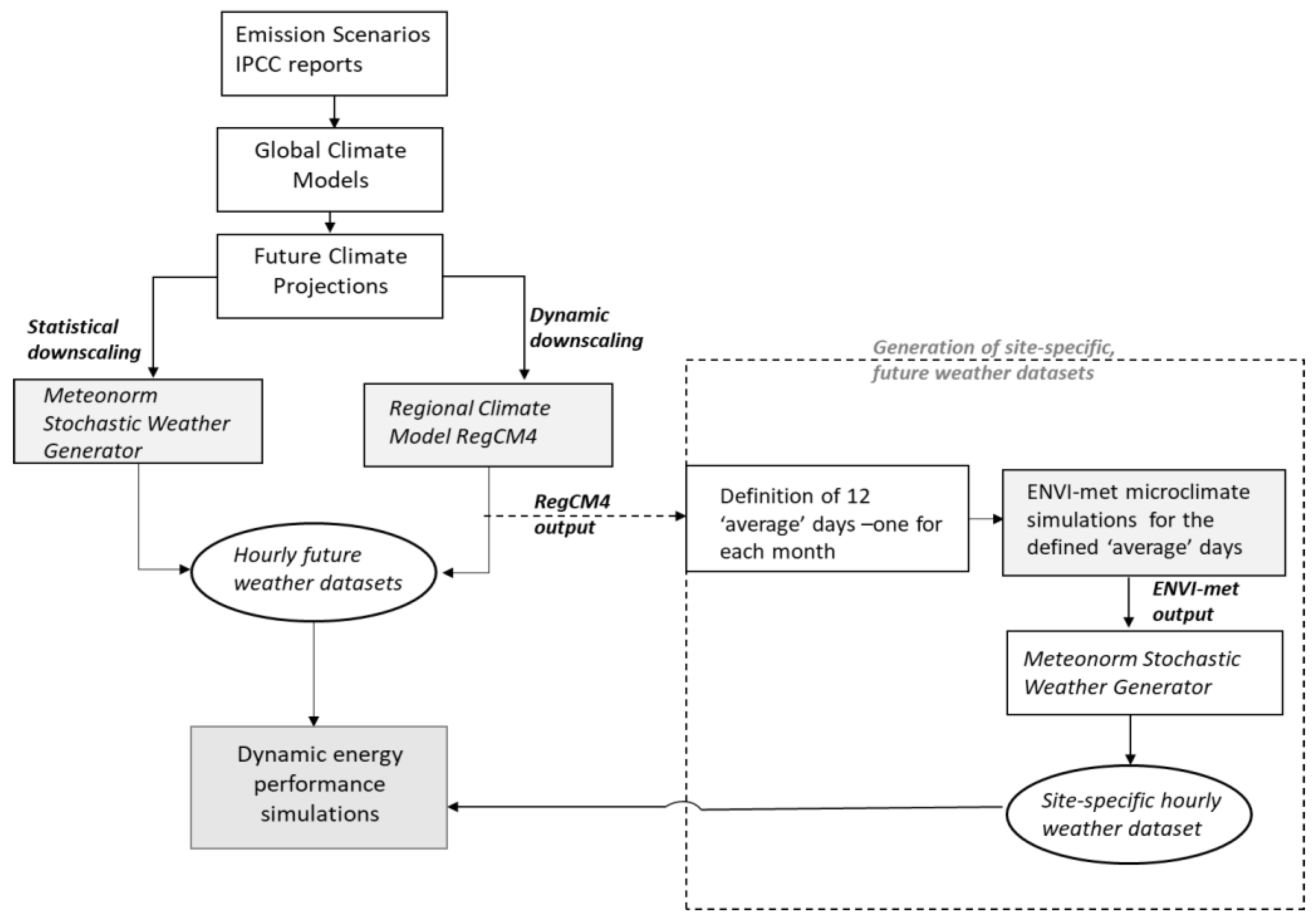
• Generate future weather datasets that account for the warming due to climate change but do not consider the site-specific microclimatic conditions and the aggravating impact of the urban warming. To this aim, the study employs both statistical and dynamical downscaling approaches for future weather file generation. Regarding the statistical downscaling, the Meteonorm Weather generator is used, while for the dynamical downscaling, the regional climate model RegCM4 is implemented.
• Create a future weather dataset that also accounts for the urban warming, intensifying the warming from climate change. Its generation will be based on the output of the regional climate model RegCM4, and the detailed methodology is presented in Section 3.1.3.
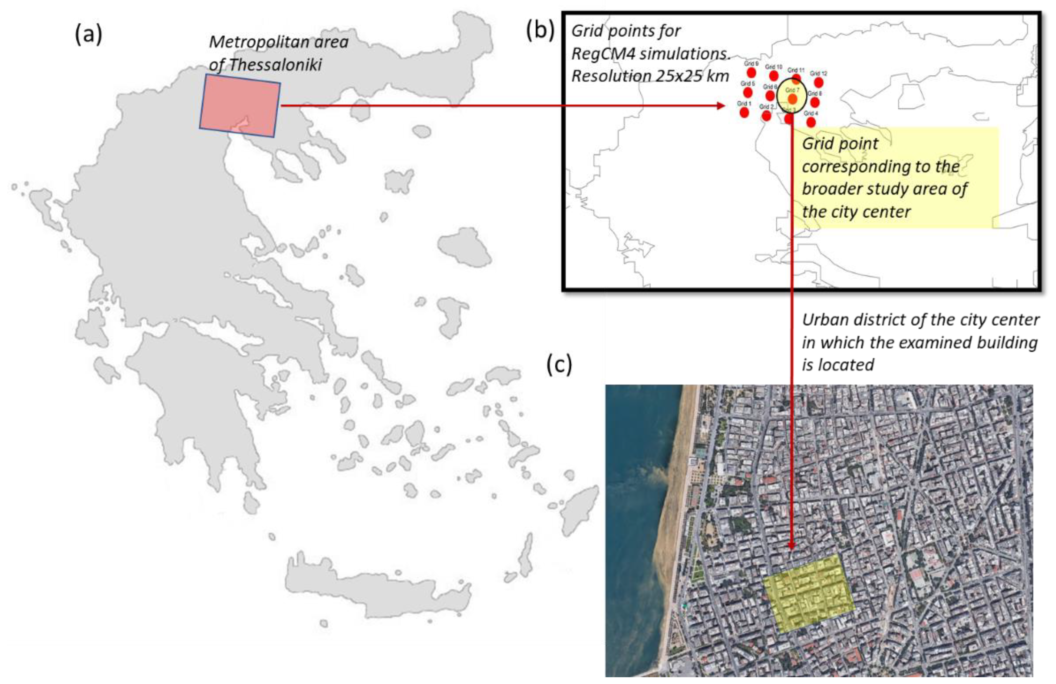
• Evaluate the impact of urban warming, caused by both climate change and the urban heat island effect, on the heating and cooling energy demand of a residential building unit located in the Mediterranean city of Thessaloniki, Greece, with the use of dynamic energy performance simulation tools.

The study is organized in the following way. As a first step, in Section 2, an overview of the most common downscaling methods of GCMs, to create future weather files for BEPS, is provided. Section 3 describes the methodology applied in this study, details on generation of weather files and the investigated building model. The results of the study are presented and discussed in Section 4, while the conclusions and the perspectives of the study are provided in Section 5.

2. Downscaling Methods of General Circulation Models (GCMs)

As previously mentioned, future emission scenarios are the main input data for the General Circulation Models (GCMs) applied for the forecasting of climate change. The various geomorphological characteristics of an area have an important role in defining the local climate. Yet, considering that the GCMs provide climate information at a rather coarse spatial resolution of 150–300 km [27] and therefore cannot represent the heterogeneity of climate variability, they must be temporally and spatially downscaled to be compatible with building energy performance simulation tools, requiring input information at finer spatial scale and at a temporal resolution of 1 h. To date, there are two main approaches to downscale GCMs: statistical and dynamical downscaling. These methods can provide high-resolution climatic information, as they model the interactions between large-scale atmospheric processes and local-scale characteristics.

2.1. Statistical Downscaling

The statistical downscaling method develops statistical relationships between observed climatic variables (often issued by historical records at a meteorological station) and larger (GCM) scale variables, employing analogue method regression analysis or stochastic methods [28]. One of the most widely applied statistical downscaling techniques is the morphing approach, a method proposed by Beclher et al. [29] to adjust present-day datasets according to future projections to be used for building energy performance simulations. The method involves the transformation or morphing of the hourly values of given weather variables of a present-day hourly weather dataset (i.e., 8760 values), based on the monthly trends and future projections, as issued by a GCM for a given location. There are three main operations for the morphing approach involving shifting, applied when an absolute change to a variable is required, the stretch or scaling factor when a relative or percentage change is predicted for a given variable, and a combination of shifting and scaling when both absolute and relative changes are predicted for a given variable. A detailed description of the morphing downscaling approach is given in [24,28,29].

Up to the present time, the morphing technique has been widely used by many researchers worldwide. Indicatively, Shen [30] employed the morphing methodology to downscale the output of GCMs and predict future hourly weather data for the period 2040–2069, to be used for dynamic energy performance simulations for residential buildings in the United States. The simulation results suggested that the expected climate change would lead to an overall reduction of the annual heating energy needs by 14.7–49% and an increase of the annual cooling energy use by 17.4–36.4%, depending on the examined climatic zone and the emission scenario. Chan [31] used the morphing method to create future hourly weather files to evaluate the effect of climate change on the energy demand of an office and a residential building in Hong Kong. The results showed that the energy consumption of the air-conditioning systems increased significantly by 2.6% to 14.3% for the office building and by 3.7% to 24% for the residential flat, depending on the emission scenario.

Wang and Chen [32] used a GCM to generate weather data for three future typical meteorological years (2020, 2050, and 2080) for 15 cities in the United States, under three emission scenarios. The obtained weather data were then downscaled using the morphing approach and they were used as an input boundary condition for the energy performance simulations of residential and commercial buildings, considered to be located at 15 different cities. The obtained results indicated that the climate change would increase the cooling energy loads for all the cities under the three CO₂ emission scenarios, whereas the heating energy demand would decrease in all cases. Still, given the climate variability from city to city, the magnitude of change considerably varied.

In the same context, Robert and Kummert [33] applied the morphing method to generate future hourly weather files to be used for the energy performance analysis of a Nearly Zero Energy Building; the results showed that, in order to obtain high-accuracy estimates of the annual energy performance of climate-sensitive buildings such as NZEBs, multi-year simulations with weather data that consider global warming and the ongoing climate change should always be performed. The simplicity and the easiness on its application has contributed to a wide use of the morphing method by the scientific community; yet, even if the generation of future weather datasets under this method leads to a similar sequence with the recorded, historical data, potential details and extremes of diurnal patterns in the future conditions cannot be captured [34].

Another method for the statistical downscaling of GCMs involves the use of stochastic weather generators that employ computer algorithms to generate long time-series of climatic parameters with statistical properties similar to existing historical climatic records. These models are very useful in cases that there are no complete datasets of all necessary weather variables as they can fill in missing data and permit the generation of long synthetic time series. A widely applied future weather generator is Meteonorm software, a weather generator that uses interpolation methods of major weather variables to provide weather data for any site in the world [35]. While Meteonorm allows access to a long database of historical time series of irradiation, temperature, humidity, precipitation and wind to create a present-day time series, it is also used for climate change studies, where the stochastic generation of the hourly time series is based on the results of IPCC’s Fourth Assessment Report (AR4) [36]. More precisely, Meteonorm combines the current databases for solar radiation and temperature and the interpolation algorithms to stochastically generate typical years for any site, for different emission scenarios and for periods up to 2100.

The Meteonorm stochastic weather generator for future weather file creation has been used in many previous studies, such as the work of Tootkaboni et al. [24] and Moazami et al. [37], who comparatively evaluated different future weather datasets and their effect on buildings’ energy performance simulations. Certainly, the use of such weather generators facilitates the generation of both present-day and future time series, especially for locations where there are not sufficient historical data. Yet, as underlined by Herrera et al., when it comes to future weather datasets, an important disadvantage is that they rely on the inherent hypothesis that future weather sequences will be similar to those observed historically [38].

2.2. Dynamical Downscaling

The dynamical downscaling refers to the use of a Regional Climate Model (RegCM), driven by the output of a GCM (used as initial and boundary conditions), to dynamically extrapolate the effects of large-scale climate processes to regional or local scales of interest [39]. RegCMs, or Limited-Area Models (LAMs), nested into GCMs can simulate “atmospheric and land surface processes, while accounting for high-resolution topographical data, land-sea contrasts, surface characteristics, and other components of the Earth-system” [40]. They can thus generate climate information at a much finer resolution than GCMs, down to 2.5–100 km, embracing in a more detailed way the topographical particularities and the climatic dynamical processes of the region of interest. On the other hand, an important disadvantage of the method relies on the considerable amount of computational power required, along with the large storage devices for the creation of the datasets [41].

Berardi et al. [23] have applied both statistical and dynamical downscaling methods to create future weather files for Canada, which have been then used for the energy performance evaluation of 16 building prototypes. Regarding the dynamic downscaling approach, the study applied the Hadley Regional Model 3 (HRM3) coupled with Hadley Climate Model 3 to create future weather files with finer spatial and temporal resolution. Based on the obtained results, the authors suggested that the higher spatial resolution of the dynamical downscaling compared to the statistical methods resulted in a better representation of the local climate conditions, leading to the higher accuracy of the dynamic buildings’ energy performance simulations. A similar conclusion was also drawn by Tootkaboni et al. [24], who comparatively assessed the effect of different future weather datasets, created both with statistical and dynamical downscaling approaches, on the dynamic energy performance analysis of typical buildings. As suggested by the authors, the statistical downscaling methods, including morphing and the stochastic approach, may provide adequate information to comparatively assess the long-term changes in energy building performance, but the dynamical downscaling method is found to be more reliable given its finer resolution.

3. Materials and Methods

3.1. Generation of Weather Datasets for Energy Performance Simulations

As previously mentioned, the scope of the study is to evaluate the role of climate change and urban microclimate on the energy performance of a generic building unit, located in Thessaloniki (40.6401° N, 22.9444° E), a city in the northern part of Greece. According to the Köppen classification, the climate of the city is Mediterranean, and it is generally characterized by hot, dry summers; mild, wet winters; and evenly distributed rainfall throughout the year [42].

To address its goal, the study employed both statistical and dynamical downscaling methods for the generation of future weather datasets. For the statistical downscaling, the stochastic weather generator Meteonorm was used, while for the dynamical downscaling, the regional climate model RegCM4 (version 4.4.5.1) was applied. Still, given that the buildings’ energy demand was strongly correlated to the microclimatic conditions of the study area, the study also aimed to generate a future weather dataset based on the outcome of the regional climate model RegCM4 that also considers the site-specific microclimatic parameters as a function of the site’s morphological parameters. More precisely, numerical simulations with RegCM4 were carried out with a horizontal grid spacing of 25 km (see Figure 2b). Yet, despite the finer spatial resolution achieved through the downscaling approaches, the microclimatic parameters of the specific case study area in which the investigated building was located (Figure 2c) cannot be considered.

To address this issue and account for the urban warming, compounding the warming due to climate change, the output of the regional climate model was used as an input boundary condition for the ENVI-met microclimate model; the microclimatic simulation results was further processed as described in the following sections and all the generated weather datasets were then used as input boundary parameters for the dynamic building energy performance simulations. The various steps to generate the future weather datasets are depicted in Figure 3 and they are described in the following sections.

3.1.1. Meteonorm Weather Generator

Meteonorm is a widely applied tool for climate data generation. It has an extensive climatic database but also offers the option of spatial interpolation for areas without any historical climatic records. Meteonorm can calculate typical years with hourly resolution for any site and its latest versions can also be used for climate change studies. More precisely, Meteonorm uses general circulation models under the fourth IPCC assessment report (AR4) and can create future weather files according to different IPCC emission scenarios (B1, A1B and A2) for intervals of 10 years between 2010 and 2100 [43]. In this study, the Meteonorm version 7.2 was used to generate:

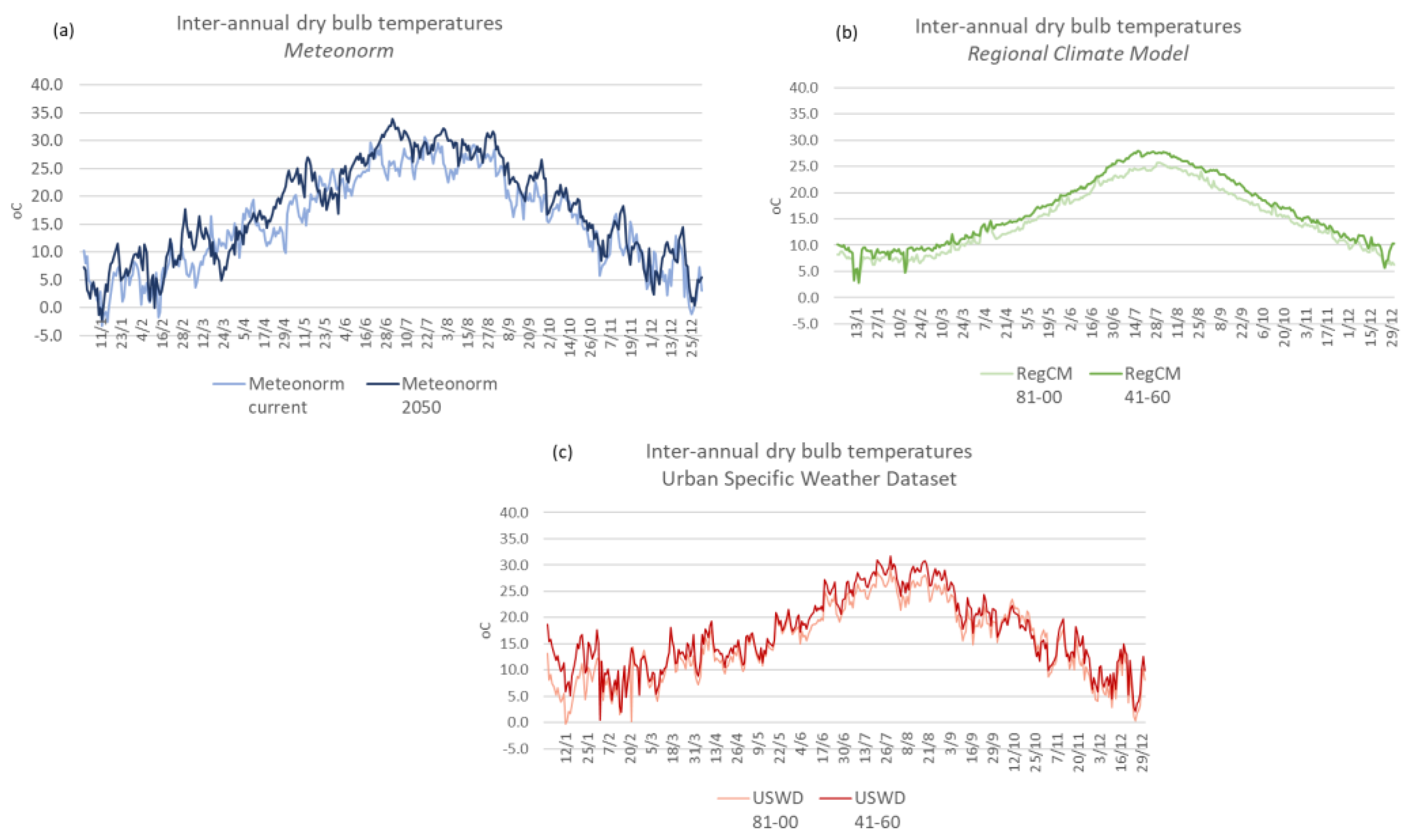
• An hourly typical weather dataset for the current period for the city of Thessaloniki (i.e., 2000), based on the irradiation database of the tool for the period 1991–2010 and the air temperature database for the period 2000–2009 (i.e., Meteonorm 2000).
• An hourly future weather file for the A1B emission scenario (intermediate scenario with rapid economic growth, more efficient technologies and a balanced use of energy sources) for the year 2050 (i.e., Meteonorm 2050).

3.1.2. Regional Climate Model RegCM4

To generate a future weather file using a regional climate model, the RegCM4 (version 4.4.5.1), a hydrostatic, compressible with sigma-p vertical coordinate model, was used [44,45,46]. The model was originally developed by the National Center for Atmospheric Research (NCAR) and its dynamical core is similar to that of the hydrostatic version of the NCAR-PSU Mesoscale Model version 5 (MM5) [47]. The spatial resolution of the model was 25 × 25 km. The simulation was driven by the HadGEM2 general circulation model (GCM), and for the future projections the model was using RCP4.5 scenario, which is an intermediate pathway with no exceedance of radiative forcing at a stabilization level of ~4.5 W/m². The main purpose of Representative Concentration Pathways is to provide time-dependent projections of atmospheric greenhouse gas concentrations [48]. In

Table 1. Configuration parameters of the RegCM4 model.

Configuration Parameter	Reference
Driving Field	HadGEM2
RCP (Future Scenario)	RCP4.5
Cumulus Scheme	Grell (over land) [49] MIT-Emanuel (over ocean) [50]
Convective Closure Scheme	Fritsch—Chappell [51]
Planetary Boundary Layer Scheme	UW Planetary Boundary Layer [52]
Ocean Flux Scheme	Zeng et al. [53]
Land Surface Model	Biosphere—Atmosphere Transfer Scheme [54]

, the main physics parameterizations of the model are presented, while further details are also provided in the work of Velikou et al. [3]. The simulation covers the period 1981–2000 (current period) and the future period 2041–2060.

Two weather files were created according to the RegCM4 output:

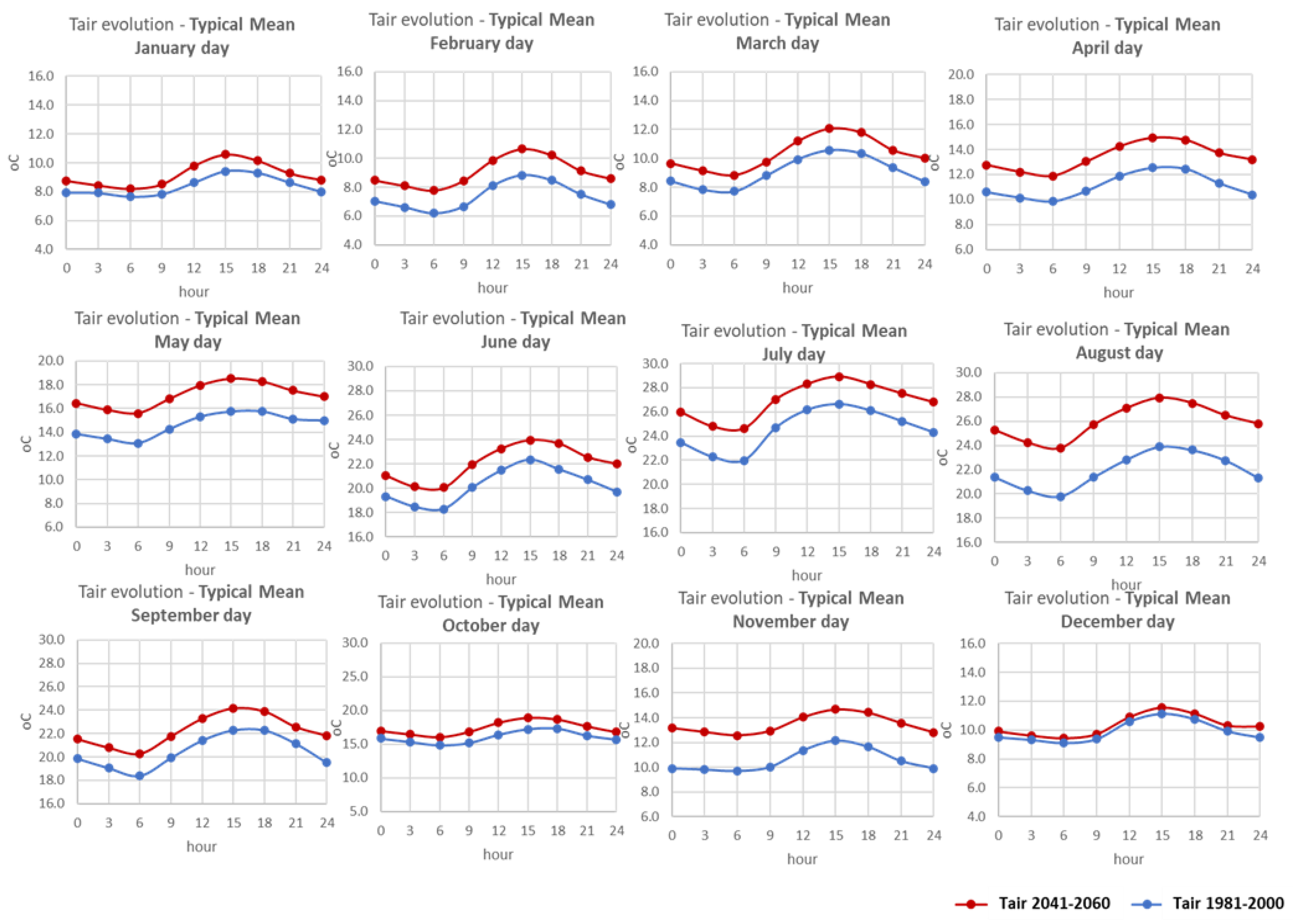
• An hourly weather file, corresponding to the present-day climatic conditions and issued by the simulation period 1981–2000 (i.e., RegCM 81-00).
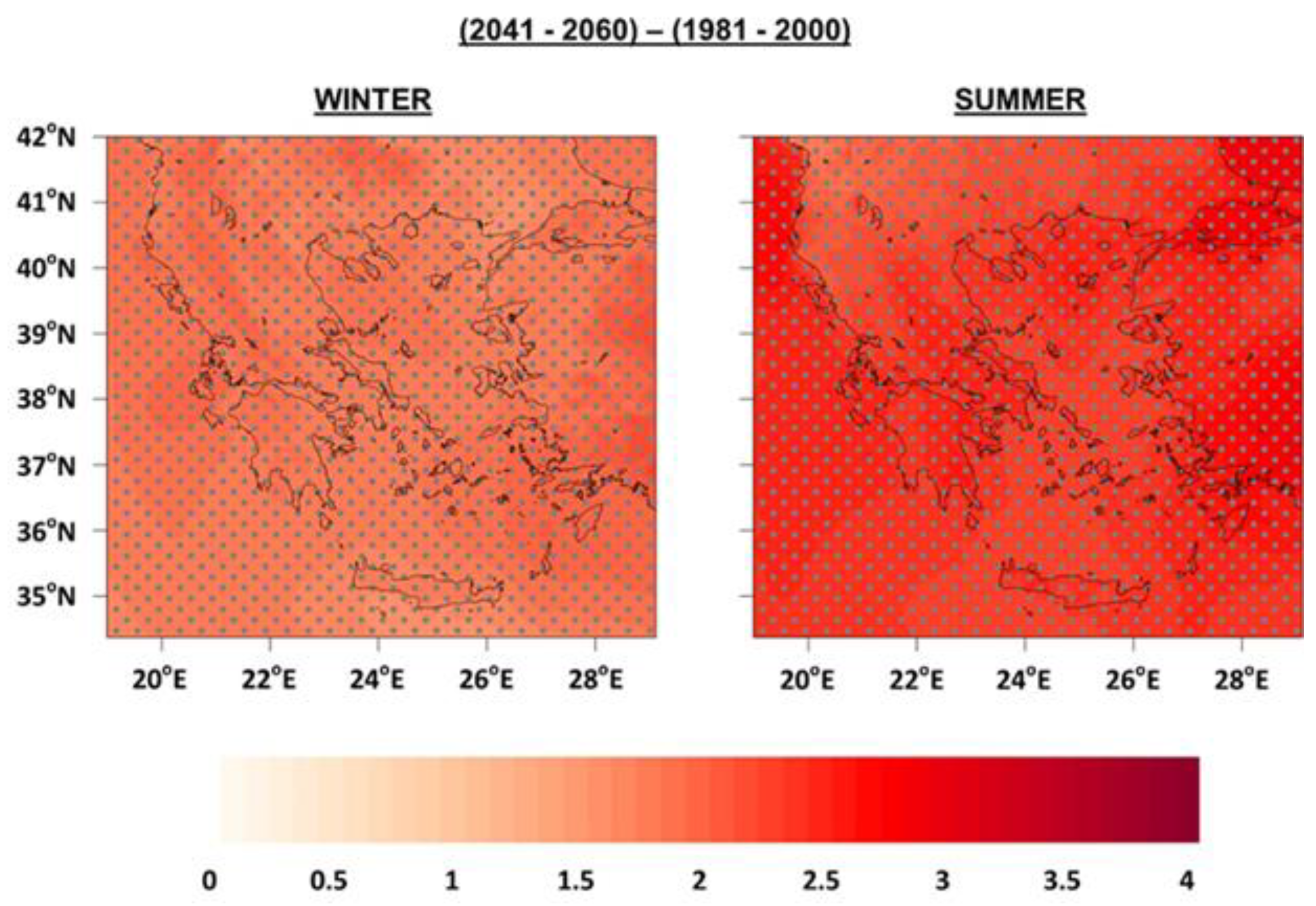
• An hourly weather file, reflecting the future climatic conditions for the period 2041–2060 (i.e., RegCM 41-60).

To this aim and for every simulation run of the RegCM4, five meteorological parameters were extracted from the corresponding grid point, which was closest to the center of Thessaloniki, where the examined building is located. These parameters included the air temperature, the relative humidity, the wind speed and the global solar radiation. At the next step, RegCM4-extracted data for periods of 1981–2000 and 2041–2060 were organized and averaged for the 20-year period to generate a single weather file of 8760 values for each period. In parallel, given that the RegCM4 simulation output included 3-hourly temporal resolution data, linear interpolation was used to estimate the hourly values for each meteorological parameter for both periods of 1981–2000 and 2041–2060. A similar approach has been also followed by Berardi et al. [23]. Finally, the obtained 8760 hourly values of each meteorological parameter and for both periods were introduced in Elements [55], an open-source platform for editing and creating custom EPW weather files, compatible with EnergyPlus dynamic building energy modeling.

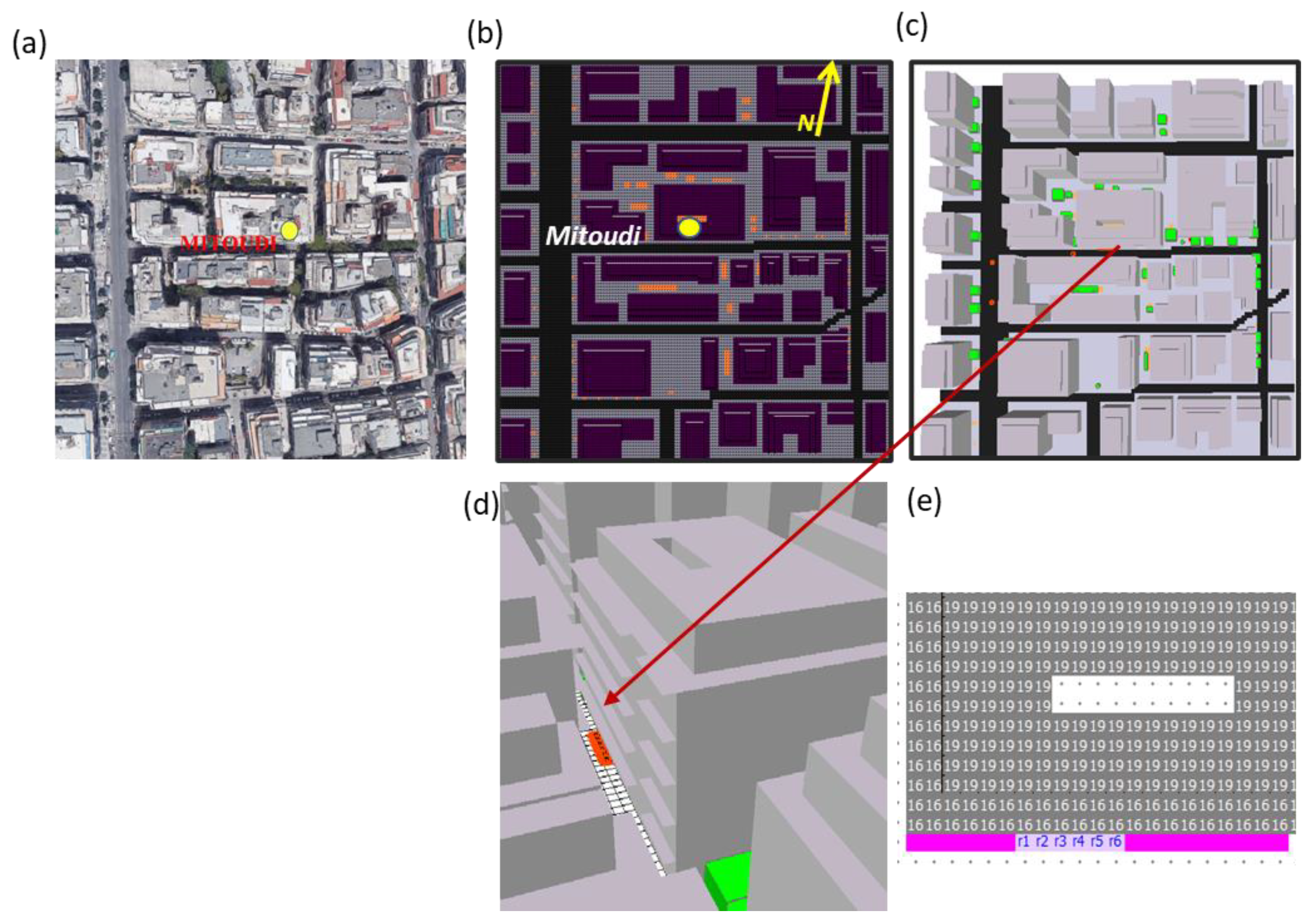
3.1.3. Microclimatic Hourly Weather File

As previously mentioned, a third type of future weather dataset was created, considering not only the general climatic conditions but also the microclimatic parameters of the examined case study area in which the investigated building unit is located. More precisely, the urban microclimate’s effect, compounding the warming due to climate change, was explored through the three-dimensional dynamic microclimatic ENVI-met v.4 model and the input boundary conditions were based on the output of the RegCM4, as obtained by the simulation described in Section 3.1.2. For the sake of comparison, simulations of the microclimatic conditions were performed for 12 typical mean days, both for the present-day conditions (i.e., 1981–2000) and the future period (2041–2060).

At this point, the following remark should be made: Based on the existing literature, for the creation of typical climatic datasets for building energy performance simulations, several years of meteorological values are needed; yet, considering the high computational cost of microclimate simulations, it would have been extremely inefficient to simulate all diurnal cycles of the periods 1981–2000 and 2041–2060 to obtain the corresponding long-term microclimatic results. To overcome this limitation, in this study each one of the 12 months was represented by a typical mean day, which was derived through the statistical analysis of the long-term data. The microclimate analysis was performed for the 12 typical mean days and based on the results the specific weather dataset was generated using Meteonorm, a synthetic year generation model that creates time series of hourly data through the utilization of stochastic methods.

More specifically, Meteonorm utilizes stochastic methodologies to generate the daily and hourly values of the most important weather variables (i.e., dry bulb temperature, relative humidity, global radiation and wind speed) on the basis of their monthly average values. The derived values have the same statistical properties as the monthly imported ones, i.e., average value, variance and characteristic sequence.

In this study, the input averages were provided by the ENVI-met microclimate simulation results for the selected typical days. The detailed approach for the creation of site-specific climatic datasets is described in [56].

All necessary meteorological boundary conditions for each simulation day were derived from the RegCM4 output. Finally, for both periods (i.e., present day and future projections), the simulated hourly microclimatic parameters were organized and processed to generate site-specific hourly weather datasets for the dynamic energy performance simulations of the next steps of the research. In this way, the generated EPW for the dynamic energy performance simulations did not involve the general climatic parameters, but the microclimatic conditions under the future climate projections; both climate change and morphological parameters of the study area were thus considered.

The methodology to create the Urban Specific Weather Datasets (USWDs), both for the current and the future climatic conditions, was based on the following steps.

• 1st step: Definition of the typical mean days for microclimate simulation

Based on the output of the RegCM4 and the simulations for both periods, as described in Section 3.1.2 (i.e., 1981–2000 and 2041–2060), the long-term average hourly values of the air temperature, relative humidity and wind speed for every month of each examined period were calculated. At the next step, these parameters will constitute the input boundary conditions for the ENVI-met microclimate simulations. Figure 4 and Figure 5 depict the hourly air temperature and relative humidity evolution for each typical mean day of all months for the periods 1981–2000 and 2041–2060. In terms of wind speed, the average daily values during the mean typical days, as derived by the analysis of the RegCM4 output for both periods, are given in

Table 2. Daily average wind speed for the mean typical days of each month and simulation period, used in ENVI-met microclimate simulations.

1981–2000
	January	February	March	April	May	June	July	August	September	October	November	December
Ws (m/s)	6.5	6.4	6.3	5.7	4.8	4.4	4.7	4.8	5.14	5.85	6.32	6.7
2041–2060
	January	February	March	April	May	June	July	August	September	October	November	December
Ws (m/s)	6.7	6.4	6.2	5.6	5.11	4.54	4.7	5.0	5.6	5.9	6.4	6.5

.

• 2nd step: ENVI-met microclimate simulations

Microclimate simulations for the case study area, in which the examined building unit is located, were conducted with the ENVI-met v.4 microclimate model, a prognostic, three-dimensional, grid-based microclimate model that can simulate the interactions of the urban surface, vegetation and the atmosphere [57]. The model contains (a) the one-dimensional (1D) boundary model, used for the initialization of the simulation and the definition of the boundary model conditions, (b) the 3D core model, consisting of 3D cells that represent different elements, such as buildings, vegetation or atmosphere. A detailed overview of the model’s characteristics, along with its limitations and advantages, is given in [58] and [59].

In this study, a total of 24 simulation runs were performed, one for each mean typical day for the two simulation periods. The study area was modeled using a domain size of 135 × 135 × 20 grids (i.e., x-grids × y-grids × z-grids), corresponding to a grid size of 1.5 m × 1.5 m × 3.0 m. Seven nesting grids were also set around the model domain area in order to assure numerical stability [60]. The ground properties of the nesting grids were those of concrete pavements to approximate in a realistic way the surfaces on the boundaries of the study area. Simulation start time was set to 00:00 and the total runtime was 24 h. The thermal properties of the various construction materials were based on the ISO standard 10,456 [61]. The Google Earth image of the study area, along with the indication of the location of the examined building unit, are shown in Figure 6. It must be also emphasized that the performance of the ENVI-met model to accurately reproduce the microclimatic characteristics of the specific case study area has been evaluated and verified in [62] and [63].

• 3rd step: Extraction of the microclimate simulation output and generation of the hourly weather datasets

The proposed computational method to consider the urban microclimate, compounding the climate change and its overall effect on the dynamic energy performance simulations, was applied for a third-floor generic building unit located inside the main street canyons of the case study area (i.e., Mitoudi canyon). The height of the base-floor was considered equal to 4.5 m, whereas the height of the remaining floors was equal to 3.0 m. Five “receptors” were considered at a distance of 0.75 m away from the façade (Figure 6d,e), which provided the values of all major microclimatic parameters at different heights, from the ground level until the top of the model domain. In our case, the results focused on air temperature (Tair), relative humidity (RH), wind speed (WS) and solar radiation (SR), on the basis of which the hourly climatic dataset was stochastically generated. For the examined third-floor building unit, the analysis concerned the heights of 10.5 m and 13.5 m. The obtained values of the studied parameters were then averaged and inserted as input data in the Meteonorm weather generator to create the two site-specific weather datasets:

• the first one reflects the microclimatic conditions occurring near the examined building unit under the present-day climatic conditions (i.e., USWD _81-00),
• the second one reflects the microclimatic conditions in the near vicinity of the examined building unit under the impact of the forecasted climate change (i.e., USWD_41-60).

3.2. Energy Performance Simulations

The following step involves the energy performance analysis using the generated hourly weather datasets for the current (i.e., Meteonorm 2000, RegCM_81-00 and USWD_81-00) and the future climatic conditions (i.e., Meteonorm 2050, RegCM_41-60 and USWD_41-60). In this study, the energy performance analysis was conducted with the EnergyPlus model [64], a tool that has been widely validated and applied in numerous scientific studies worldwide [65,66]. In EnergyPlus, the calculation of the thermal loads of buildings is based on the heat balance method, while accounting for the heat fluxes on outdoor and indoor surfaces, and the transient heat conduction through the building elements [64]. The plan of the investigated building unit has a total surface of 80 m². The 3D model of the zone in the EnergyPlus model along with its surrounding obstacles are shown in Figure 7a–c, respectively. It is assumed that the floor, the ceiling and all vertical surfaces of the building unit, except for the main façade, are regarded as adiabatic, due to the same operational schedules between the apartments. The exposed façades are facing South. All simulations were conducted for the existing building envelope, in which there is no thermal insulation. In fact, the building containing the investigated building unit was constructed prior of 1979, in a period when there were no specific requirements for the thermal protection of the building. Up to the present time, the highest part of the Hellenic building stock was built during this period and thus, the envelope components are poorly insulated or not insulated at all. Regarding the examined building, the opaque external building wall towards the external air consists of brick masonry with U = 1.64 W/m²K. The bearing vertical components, consisting of reinforced concrete, presented U values between 2.53 W/m²K and 3.17 W/m²K, depending on their width. Similarly, the brick wall and the reinforced concrete components, facing towards the non-conditioned staircase area, presented U values of 1.43 W/m²K and 2.06 W/m²K–2.46 W/m²K, respectively. Regarding the openings, the thermal transmittance of the PVC frame was Uf = 2.8 W/m²/K, the double-glazed glass conductance was equal to Ug = 2.8 W/m²/K.

In parallel, the operational profile of the generic building unit, which includes the schedules for occupancy, lighting, equipment, ventilation, infiltration, as well as the heating and cooling setpoints, was defined in accordance with the national regulatory framework for the building energy performance [67].

The heating season covers the period of the 15 October to the 30 April, whereas the cooling season starts 1 June and ends 31 August. Moreover, different heating and cooling setpoints were considered to examine the potential energy savings that can be achieved due to the thermostat adjustment. The base case setpoint range proposed by the national building energy performance regulation for residential buildings and building units is 20–26 °C. In this study, the heating setpoint was initially fixed at 20 °C, while the cooling setpoint was considered as 26 °C and 27 °C. In the next step, the heating setpoint was fixed at 19 °C, while the cooling setpoint was considered at 26 °C and 27 °C. The infiltration rate was 1.0 ACH. Finally, in the summer period, a night ventilation rate of 3ACH was considered, provided that the indoor air temperature is higher than the outdoor air temperature by 1.0 °C.

4. Results and Discussion

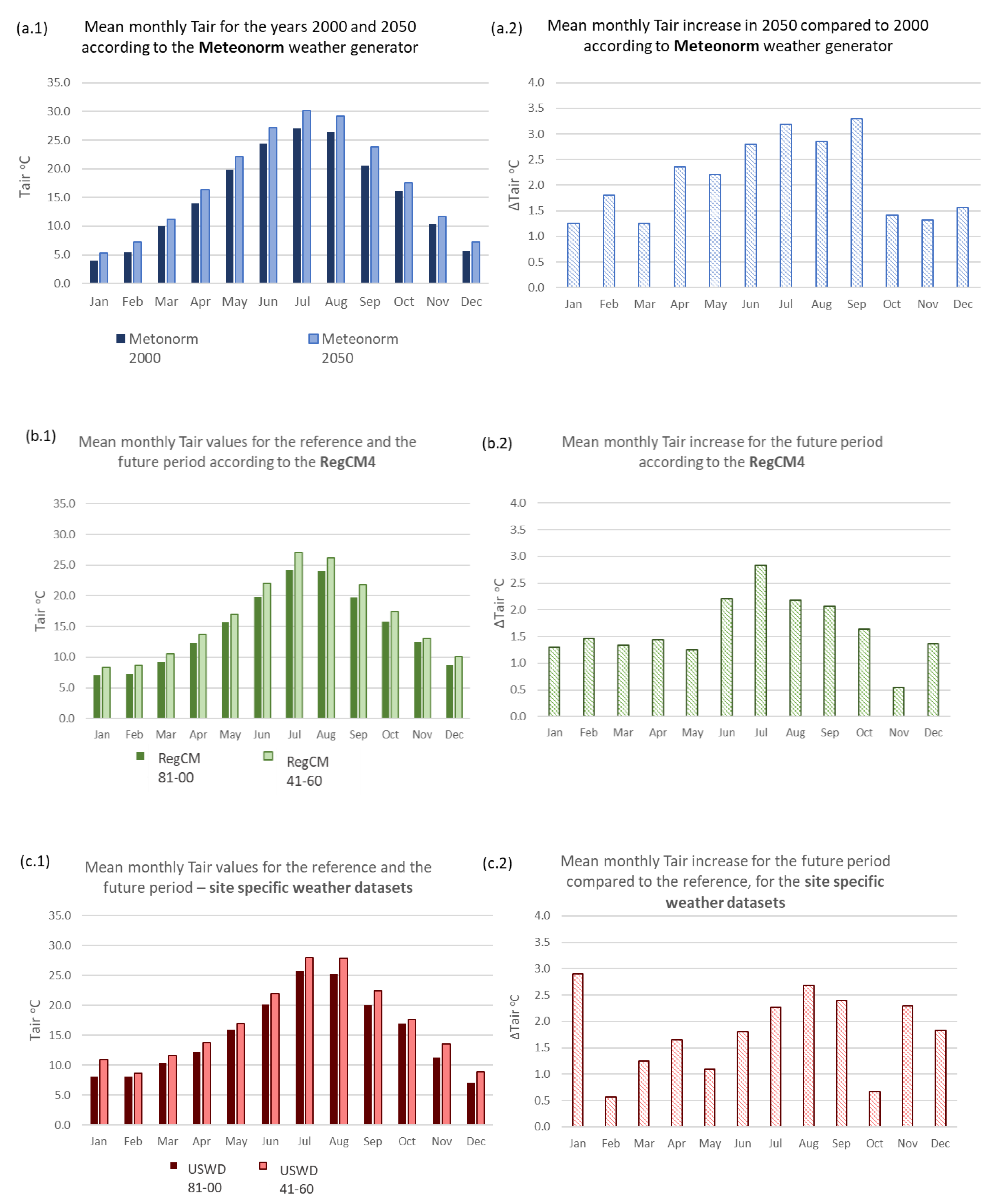
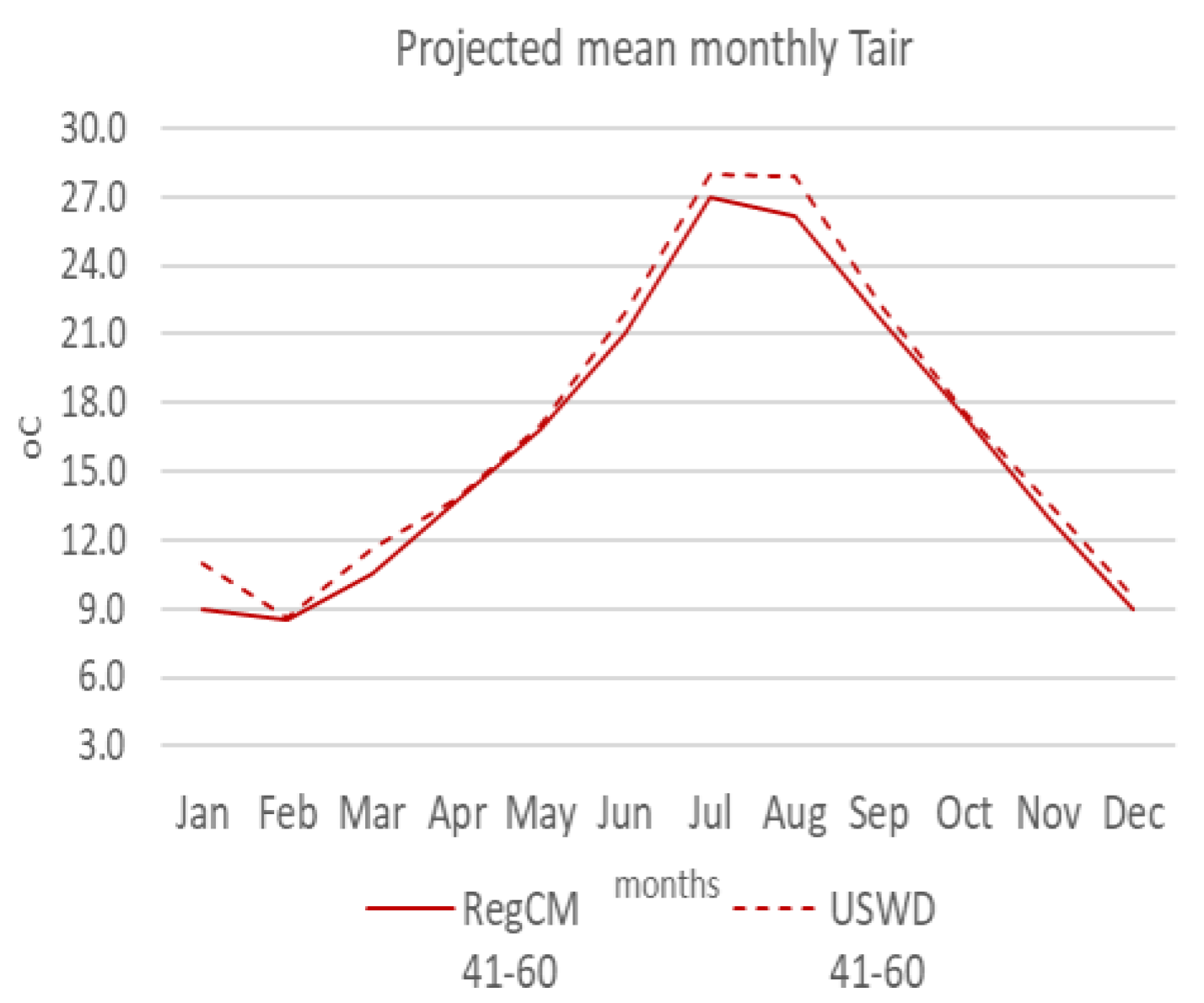
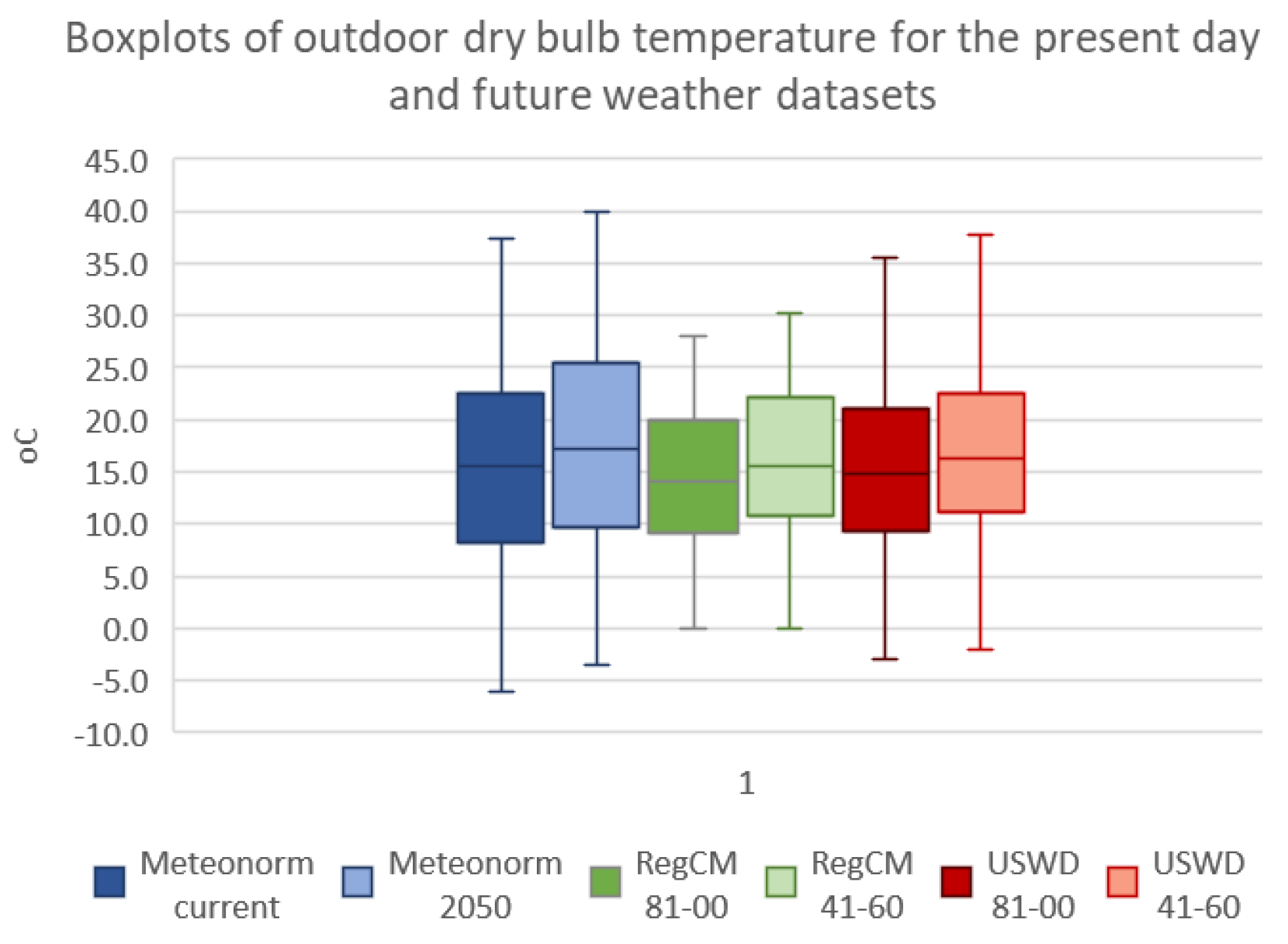
4.1. Weather File Analysis

The analysis of the air temperature between the present day and the future weather datasets on a daily basis throughout the year showed that in all the examined cases, the generated datasets follow a similar inter-annual profile, with the future ones presenting higher Tair values, depicting the impact of climate change on the created weather files. Regarding the datasets generated with statistical downscaling methods, the range of the daily Tair varies between −3.3 °C to 30.7 °C and −2.1 °C to 33.9 °C for the reference (i.e., Meteonorm 2000) and the future period (i.e., Meteonorm 2050), respectively (Figure 8a). In terms of the annual weather files generated using the RegCM4 output, the range of the daily air temperature fluctuates between 2.7 °C to 25.62 °C and 2.83 °C to 27.9 °C for the reference (i.e., RegCM_81-00) and the future period (i.e., RegCM_41-60), respectively (Figure 8b). With the urban heat island effect compounding the warming due to climate change, the maximum future daily Tair value was estimated at 31.6 °C (i.e., USWD 41-60), which is higher by 3.7°C when compared to the scenario where the site-specific microclimatic parameters are not accounted for. Aiming for a more thorough analysis of the results, the mean monthly values of all future and present-day datasets were calculated; as can be seen in Figure 9, the future weather file generated with Meteonorm forecasts a mean monthly temperature increase between 1.3–1.8 °C and 2.2–3.3 °C during the heating and cooling period, respectively. Peak maximum values, surpassing 3.0 °C, are estimated for the months of July and September. The same tendency is also reported for the future projections with the RegCM4, estimating an increase in the mean monthly Tair by 2.1–2.8 °C during the summer months of the year and an average increase of 1.4 °C during winter months.

To continue, Figure 10 shows the projected mean monthly Tair values for the period 2041–2060, with and without the consideration of the site-specific microclimatic conditions and the compounding impact of the urban warming. As it can be seen, with the heat island effect intensifying the warming from climate change, higher mean monthly Tair values are to be expected in the future period 2041–2060. The air temperature values of USWD_41-60 are generally higher than the RegCM_41-60 ones, with the largest differences detected in summer; in fact, the mean future monthly Tair values inside the urban district will reach 28.1 °C and 27.9 °C in July and August, i.e., 1.1 °C and 1.7 °C higher compared to the scenario where only the climate change is accounted and not the local microclimate of the dense urban area. The lowest differences were noticed in the intermediate seasons (i.e., autumn and spring) ranging between 0.2 °C and 0.6 °C. The reported discrepancies between the two weather datasets are the result of complex microclimatic conditions, which are reproduced by the ENVI-met model and are mainly attributed to (i) the increased building density of the study area which lowers the longwave radiation losses, (ii) the thermal properties of the construction materials, which contribute to the storage and emittance of sensible heat to the air, and (iii) to the reduced green areas, which lead to lower amounts of latent heat.

Finally, the boxplots of the outdoor Tair for all generated weather datasets show a clear increase in the future temperatures (Figure 11). However, as also previously mentioned, the projections for the future climate change are considerably higher for the weather file developed with Meteonorm generator using statistical downscaling methods compared to the RegCM_41-60 and the USWD_41-60, the generation of which is based on dynamical downscaling approaches. The lower dispersion of data in cases where future weather files have been generated with dynamical downscaling methods compared to datasets derived from statistical downscaling methods has also been mentioned in previous scientific studies of Tootkaboni et al. [27] and Berardi et al. [23].

The higher differences produced by the statistical downscaling methods compared to the dynamical approaches are strongly associated with the different algorithms and spatial representativeness followed at each case. More precisely, the RegCM4 numerically solves the governing equations of the atmosphere in a limited spatial domain, driven by the input boundary conditions of a General Circulation Model, while on the other hand, statistical downscaling models develop statistical relationships between observed climatic variables at a specific point station (i.e., historical records at a meteorological station) and model variables. In other words, there are considerable differences on the spatial representativeness of the two approaches, with the RegCM4 providing results at an area that corresponds to the model grids, while the statistical downscaling models provide results at point stations driven by the historical observations [68,69]. Apart from the different spatial representativeness, another important parameter that contributes to the variability of the projected climatic data is associated with the different emission scenarios; RegCM4 used the RCP4.5 scenario, introduced in the Fifth IPCC Assessment Report, whereas Meteonorm, the statistical downscaling model, uses the fourth IPCC assessment report (AR4) scenarios and more precisely, the A1B, an intermediate scenario. Despite the close analogues between the SERS scenarios and the RCP scenarios, their creation follows a different approach, thus leading to diverse climatic projections. Relevant comparisons have been already performed in the literature, such as the work of Farag et al. [70] who comparatively assessed the SRES and RCP scenarios for temperature forecasting under different climatic regions in Egypt. As the next step, the generated present-day and future weather datasets are used as input boundary condition for the dynamic energy performance simulations of the investigated building unit.

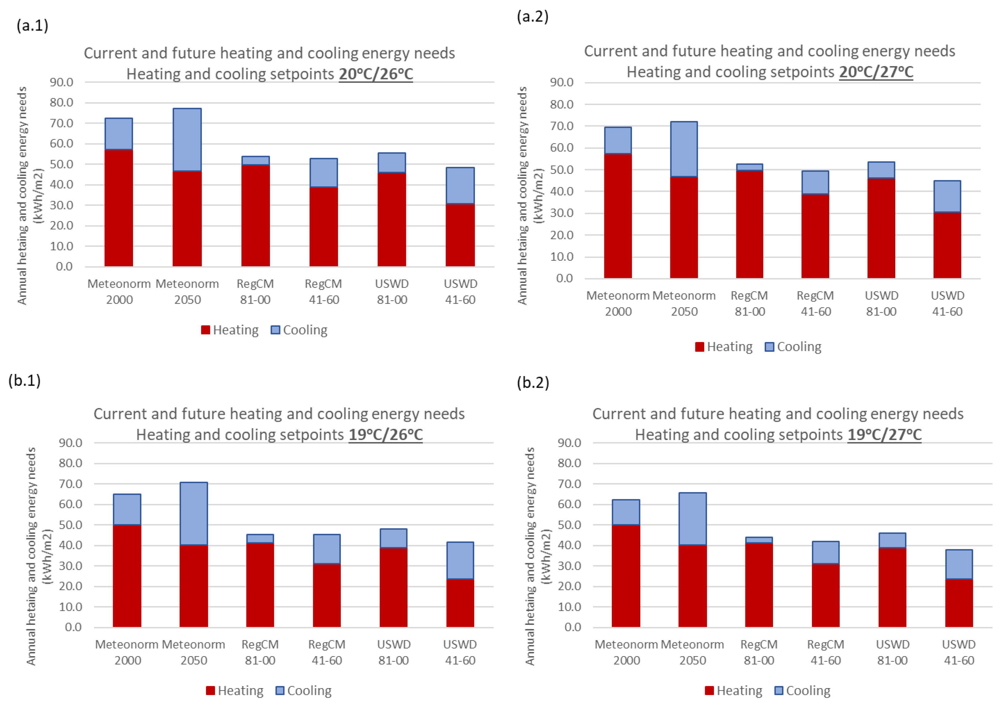
4.2. Building Energy Performance Simulation Results

Figure 12 presents the annual heating and cooling energy needs of the examined building unit in Thessaloniki estimated for all the generated weather datasets, according to the current and future climate conditions and for different heating and cooling setpoints. As it can be seen, in all cases the heating energy demand dominates over the cooling energy needs, which is expected due to the geographical position and the climate of the region. Yet, there is an increasing trend in cooling energy requirements and a reduction in the heating needs for the future, with the projected changes varying according to the technique used for the generation of the weather dataset and the corresponding magnitude of temperature increases in summer and winter.

The first run of EnergyPlus simulations was performed for the heating and cooling setpoints of 20 °C and 26 °C, respectively, following the Provisions of the National Building Energy Performance Regulation. As depicted in Figure 12a.1, an increase of 6.5% on the total heating and cooling energy needs is forecasted for the Meteonorm weather files, while the respective change is marginal for the RegCM4 future weather files and did not exceed 2%.

Moreover, the annual heating energy demand for the future period 2050 is projected to decrease by 18.5% (−10.6 KWh/m²), whereas the cooling energy demand is expected to be doubled (+15.64 KWh/m²) for the Meteonorm weather files. On the other hand, lower changes on the future cooling energy needs (i.e., an increase by 9.70 KWh/m²) are forecasted for the RegCM4 future weather file, mainly due to the smaller projected Tair increase and the lower dispersion of temperature values compared to the Meteonorm files. Regarding the heating energy demand for the future period 2041–2060 for the RegCM4 dataset, a decrease by 10.70 KWh/m² (i.e., 21.0%) was projected, a value that is close to the one forecasted with the Meteonorm weather dataset.

To evaluate the intensifying combined effect of climate change and urban microclimate on the urban warming and the building’s energy demand, EnergyPlus dynamic simulations were conducted using the generated USWDs (i.e., USWD_81-00 and USWD_41-60). According to the obtained simulation results, the consideration of the local microclimate in the dynamic energy performance simulations resulted in an overall future heating and cooling energy demand of 48.45 kWh/m², which is 8% compared to the respective value obtained for the RegCM4 dataset (i.e., when only the climate change impact is accounted for). In parallel, the simulation results indicated that when the local microclimate was not considered and only the climate change was taken into account, the annual heating energy demand for the present-day and the future conditions was overestimated by 7.5% and 21%, respectively. Similarly, the cooling energy demand, both for the current and the future climatic conditions, was considerably underestimated when the higher urban air temperatures were not accounted for. In fact, when the combined effect of climate change and urban warming was considered in the energy performance simulations (i.e., simulation run with the USWD_41-60), the annual cooling energy needs of the building unit were estimated to be 17.8 KWh/m² or 22.4% higher compared to the results obtained only under the climate change effect (i.e., simulation run with the RegCM_41-60).

The important increase of future energy needs for cooling purposes is expected to lead to a substantial increase in electricity use in urban areas of cities such as Thessaloniki, characterized by rather warm climatic conditions. Given that in residential buildings the cooling demand constitutes the highest part of the total electricity consumption compared to lighting and equipment, the high urban air temperatures due to climate change and urban heat island are expected to exacerbate the peak cooling energy loads, shifting the peak electricity demand upwards and stressing the electricity infrastructure.

A simple way to reduce the future cooling energy demand, while also assuring the indoor thermal comfort conditions would be to set a different, higher cooling setpoint, which in this study can be defined at 27 °C. Figure 12a.2 presents the current and future energy needs for heating/cooling setpoints of 20 °C/27 °C. As it can be seen, increasing the cooling setpoint by 1.0 °C may contribute to a further reduction of the present-day and future cooling energy demand by 18% and 17%, respectively, for Meteonorm weather files; similarly, the cooling setpoint of 27 °C rather than 26 °C would contribute to a 23% and 20% decrease (i.e., 3.0 KWh/m² and 3.8 KWh/m²) on the future cooling energy needs for the RegCM4_41-60 and USWD_41-60 weather datasets, correspondingly.

Regarding the effect of the increase of the cooling setpoint by 1.0 °C on the present day, total annual energy demand (i.e., sum of heating and cooling), a decrease of 4%, 6% and 3.9% has been estimated for the Meteonorm, RegCM4 and USWD weather files. In terms of the future total annual energy needs, when the cooling setpoint is increased by 1 °C while maintaining the heating setpoint to 20 °C, the maximum total energy savings reached 6.7%, 6.0% and 7.5% for the Meteonorm, RegCM4 and USWD future weather files, respectively.

To further evaluate the potential changes on the total annual energy demand, a lower heating setpoint was also examined (i.e., 19 °C). Figure 12 present the future heating and cooling energy needs for all the examined heating/cooling setpoints and for all the evaluated weather datasets. The comparison of the obtained simulation results between the heating/cooling setpoints scenario of 19 °C/26 °C and the base case scenario (i.e., 20 °C/26 °C) has led to the following remarks: Lowering the heating thermostat by 1.0 °C can result in (a) a reduction of future overall energy needs by 8.5%, 14.3% and 14.1% for the Meteonorm, RegCM4 and USWD future weather files, respectively, (b) a decrease of the future annual heating energy demand by 14%, 19.7% and 22.5% for the Meteonorm, RegCM4 and USWD future weather files, correspondingly.

Finally, as anticipated, the largest energy savings compared to the base scenario (i.e., 20 °C/26 °C) are achieved when the thermostatic setpoints are set to 19 °C/27 °C, resulting in a decrease on the energy demand by 15%, 20.8% and 21.6% for the Meteonorm, RegCM4 and USWD future weather files. It can thus be said that the reduction of the heating setpoints would lead to a more considerable energy reduction rather than the increase of the cooling setpoint, which agrees with the findings of Berardi et al. [23].

5. Conclusions

The present study evaluated the impact of climate change and urban heat island on the heating and cooling energy demand of a generic building unit in the city of Thessaloniki, Greece. As a first step, the study focused on the generation of future weather datasets using statistical and dynamical downscaling methods; regarding the statistical downscaling, the Meteonorm stochastic weather generator was employed, creating a future weather dataset for the year 2050 under the A1B scenario of the 4th IPCC report. In parallel, the use of the RegCM4 model allowed for the projection of future climate conditions under the RCP4.5 emission scenario for the future period 2041–2060. Given the significant impact of urban microclimatic parameters and the consequent urban heat island effect on the buildings’ energy demand, the study proposed a computational method to generate future weather datasets that account not only for the general climatic conditions but also for the microclimatic parameters of the examined case study area, in which the investigated building unit is located. The compounding effect of urban heat island on the warming due to climate change was explored through the three-dimensional dynamic microclimatic ENVI-met v.4 model and the input boundary conditions were based on the output of the RegCM4.

The analysis of the future weather files suggested an increase on the annual Tair for the city of Thessaloniki by 1.6–2.1 °C, with the higher values projected by the Meteonorm generator using statistical downscaling methods compared to the RegCM4 output, which employs dynamical downscaling approaches. Interestingly, the consideration of the complementary role of the site-specific microclimatic parameters of the study area resulted in a further annual Tair increase by 0.3 °C (i.e., estimated annual Tair rise of 1.9 °C, with the discrepancies being considerably high in summer).

To continue, the energy performance simulation results revealed that climate change will lead to a substantial increase of the cooling energy needs, while reducing the heating energy demand. Still, the magnitude of the modification on heating and cooling energy demand has been found to be dependent on the technique used for the future weather file generation. Again, the simulation results highlighted the importance of considering the intensifying effect of urban heat island on climate change when forecasting the future buildings’ energy demand, since its neglection may lead to an overestimation of the heating energy demand by 21% and an underestimation of the cooling energy needs by 22.4%.

To conclude, the results of the study highlight the necessity of following a holistic approach towards the evaluation of buildings’ future energy demand, accounting both for the climate change and the urban heat island phenomenon. Given that the buildings’ life cycle extends to decades, it is essential to accurately evaluate their performance over a series of years and propose design strategies that will meet the energy performance and occupants’ comfort requirements in the future. Future work should incorporate (a) the impact of the urban geometry, building orientation and the materials’ optical and thermal properties on the energy performance simulation results under different climate change scenarios, and (b) the role of various mitigation and adaptation strategies, such as the addition of nature-based solutions on the urban landscape or on the building envelope, since efforts to attenuate the heat island effect also help to address climate change and improve citizens’ quality of life. Moreover, this study only investigated the energy performance of a single building unit in Thessaloniki; future work will also incorporate building units at different levels and positioned inside street canyons with different orientations in various locations of Greece to further address the compounding role of the urban microclimate and urban heat island on climate change.

References

1. Solomon, S.; Manning, M.; Marquis, M.; Qin, D. Climate Change 2007—The Physical Science Basis: Working Group I Contribution to the Fourth Assessment Report of the IPCC; Cambridge University Press: Cambridge, UK, 2007; Volume 4. [Google Scholar]
2. Tolika, K.; Zanis, P.; Anagnostopoulou, C. Regional climate change scenarios for Greece: Future temperature and precipitation projections from ensembles of RCMs. Global NEST J. 2012, 14, 407–421. [Google Scholar]
3. Velikou, K.; Tolika, K.; Anagnostopoulou, C.; Zanis, P. Sensitivity analysis of RegCM4 model: Present time simulations over the Mediterranean. Theor. Appl. Clim. 2019, 136, 1185–1208. [Google Scholar] [CrossRef]
4. Giorgi, F. Climate Change Hot-Spots. Geophys. Res. Lett. 2006, 33, L08707. [Google Scholar] [CrossRef]
5. Tuel, A.; Eltahir, E.A.B. Why Is the Mediterranean a Climate Change Hot Spot? J. Clim. 2020, 33, 5829–5843. [Google Scholar] [CrossRef]
6. IPCC. Climate Change 2014: Synthesis Report. In Contribution of Working Groups I, II, and III to the Fifth Assessment Report of the Intergovernmental Panel on Climate Change; IPCC: Geneva, Switzerland, 2014. [Google Scholar]
7. Nakicenovic, N.; Alcamo, J.; Davis, G.; Vries, B.D.; Fenhann, J.; Gaffin, S.; Gregory, K.; Grubler, A.; Jung, T.Y.; Kram, T. IPCC Special Report on Emissions Scenarios; Cambridge University Press: Cambridge, UK, 2000. [Google Scholar]
8. Moss, R.H.; Babiker, M.; Brinkman, S.; Calvo, E.; Carter, T.; Edmonds, J.A.; Elgizouli, I.; Emori, S.; Lin, E.; Hibbard, K. Towards New Scenarios for Analysis of Emissions, Climate Change, Impacts, and Response Strategies; Technical Summary; Intergovernmental Panel on Climate Change: Geneva, Switzerland, 2008. [Google Scholar]
9. Diffenbaugh, N.S.; Pal, J.S.; Giorgi, F.; Gao, X. Heat stress intensification in the Mediterranean climate change hotspot. Geophys. Res. Lett. 2007, 34. [Google Scholar] [CrossRef] [Green Version]
10. Zanis, P.; Katragkou, E.; Ntogras, C.; Marougianni, G.; Tsikerdekis, A.; Feidas, H.; Anadranistakis, E.; Melas, D. Transient high-resolution regional climate simulation for Greece over the period 1960–2100: Evaluation and future projections. Clim. Res. 2015, 64, 123–140. [Google Scholar] [CrossRef] [Green Version]
11. Velikou, K. Dynamical Downscaling of Regional Climate Model RegCM for the Greek Region: Statistical Assessment, Dynamical Evaluation, Effects and Future Scenarios. Ph.D. Thesis, Aritotle University of Thessaloniki, Thessaloniki, Greece, 2021. [Google Scholar]
12. Akbari, H.; Cartalis, C.; Kolokotsa, D.; Muscio, A.; Pisello, A.L.; Rossi, F.; Santamouris, M.; Synnefa, A.; Wong, N.H.; Zinzi, M. Local climate change and urban heat island mitigation techniques—The state of the art. J. Civ. Eng. Manag. 2015, 22, 1–16. [Google Scholar] [CrossRef] [Green Version]
13. Kubilay, A.; Ferrari, A.; Derome, D.; Carmeliet, J. Smart wetting of permeable pavements as an evaporative-cooling measure for improving the urban climate during heat waves. J. Build. Phys. 2021, 45, 36–66. [Google Scholar] [CrossRef]
14. Arnfield, A.J. Two decades of urban climate research: A review of turbulence, exchanges of energy and water, and the urban heat island. Int. J. Clim. 2003, 23, 1–26. [Google Scholar] [CrossRef]
15. Rizwan, A.M.; Dennis, L.Y.; Liu, C. A review on the generation, determination and mitigation of Urban Heat Island. J. Environ. Sci. 2008, 20, 120–128. [Google Scholar] [CrossRef]
16. Allegrini, J.; Dorer, V.; Carmeliet, J. Influence of the urban microclimate in street canyons on the energy demand for space cooling and heating of buildings. Energy Build. 2012, 55, 823–832. [Google Scholar] [CrossRef]
17. Sanzighi, S.M.; Soflaei, F.; Shokouhian, M. A comparative study of thermal performance in three generations of Iranian residential buildings: Case studies in Csa Gorgan. J. Build. Phys. 2021, 44, 326–363. [Google Scholar] [CrossRef]
18. Ohashi, Y.; Genchi, Y.; Kondo, H.; Kikegawa, Y.; Yoshikado, H.; Hirano, Y. Influence of Air-Conditioning Waste Heat on Air Temperature in Tokyo during Summer: Numerical Experiments Using an Urban Canopy Model Coupled with a Building Energy Model. J. Appl. Meteorol. Clim. 2007, 46, 66–81. [Google Scholar] [CrossRef]
19. Gobakis, K.; Kolokotsa, D. Coupling building energy simulation software with microclimatic simulation for the evaluation of the impact of urban outdoor conditions on the energy consumption and indoor environmental quality. Energy Build. 2017, 157, 101–115. [Google Scholar] [CrossRef]
20. Liang, X.-Z.; Kunkel, K.E.; Meehl, G.A.; Jones, R.; Wang, J.X.L. Regional climate models downscaling analysis of general circulation models present climate biases propagation into future change projections. Geophys. Res. Lett. 2008, 35, 8. [Google Scholar] [CrossRef] [Green Version]
21. Zhu, M.; Pan, Y.; Huang, Z.; Xu, P. An alternative method to predict future weather data for building energy demand simulation under global climate change. Energy Build. 2016, 113, 74–86. [Google Scholar] [CrossRef]
22. Xu, P.; Huang, Y.J.; Miller, N.; Schlegel, N.; Shen, P. Impacts of climate change on building heating and cooling energy patterns in California. Energy 2012, 44, 792–804. [Google Scholar] [CrossRef]
23. Berardi, U.; Jafarpur, P. Assessing the impact of climate change on building heating and cooling energy demand in Canada. Renew. Sustain. Energy Rev. 2020, 121, 109681. [Google Scholar] [CrossRef]
24. Tootkaboni, M.P.; Ballarini, I.; Corrado, V. Analysing the future energy performance of residential buildings in the most populated Italian climatic zone: A study of climate change impacts. Energy Rep. 2021. [Google Scholar] [CrossRef]
25. Attia, S.; Gobin, C. Climate Change Effects on Belgian Households: A Case Study of a Nearly Zero Energy Building. Energies 2020, 13, 5357. [Google Scholar] [CrossRef]
26. Yassaghi, H.; Hoque, S. An Overview of Climate Change and Building Energy: Performance, Responses and Uncertainties. Buildings 2019, 9, 166. [Google Scholar] [CrossRef] [Green Version]
27. Tootkaboni, M.P.; Ballarini, I.; Zinzi, M.; Corrado, V. A comparative analysis of different future weather data for building energy performance simulation. Climate 2021, 9, 37. [Google Scholar] [CrossRef]
28. Guan, L. Preparation of future weather data to study the impact of climate change on buildings. Build. Environ. 2009, 44, 793–800. [Google Scholar] [CrossRef]
29. Belcher, S.E.; Hacker, J.N.; Powell, D.S. Constructing design weather data for future climates. Build. Serv. Eng. Res. Technol. 2005, 26, 49–61. [Google Scholar] [CrossRef]
30. Shen, P. Impacts of climate change on U.S. building energy use by using downscaled hourly future weather data. Energy Build. 2017, 134, 61–70. [Google Scholar] [CrossRef]
31. Chan, A. Developing future hourly weather files for studying the impact of climate change on building energy performance in Hong Kong. Energy Build. 2011, 43, 2860–2868. [Google Scholar] [CrossRef]
32. Wang, H.; Chen, Q. Impact of climate change heating and cooling energy use in buildings in the United States. Energy Build. 2014, 82, 428–436. [Google Scholar] [CrossRef] [Green Version]
33. Robert, A.; Kummert, M. Designing net-zero energy buildings for the future climate, not for the past. Build. Environ. 2012, 55, 150–158. [Google Scholar] [CrossRef]
34. Jentsch, M.; Bahaj, A.S.; James, P.A. Climate change future proofing of buildings—Generation and assessment of building simulation weather files. Energy Build. 2008, 40, 2148–2168. [Google Scholar] [CrossRef]
35. Remund, J.; Müller, S. Solar Radiation and Uncertainty Information of Meteonorm 7. In Proceedings of the 26th European Photovoltaic Solar Energy Conference and Exhibition, Hamburg, Germany, 5–9 September 2011; pp. 4388–4390. [Google Scholar]
36. Remund, J.; Müller, S.; Schilter, C.; Rihm, B. The Use of Meteonorm Weather Generator for Climate Change Studies. In Proceedings of the 10th EMS Annual Meeting, Zürich, Switzerland, 3–10 September 2021; EMS: Barcelona, Spain, 2010; p. EMS2010-417. [Google Scholar]
37. Moazami, A.; Nik, V.M.; Carlucci, S.; Geving, S. Impacts of future weather data typology on building energy performance—Investigating long-term patterns of climate change and extreme weather conditions. Appl. Energy 2019, 238, 696–720. [Google Scholar] [CrossRef]
38. Herrera, M.; Natarajan, S.; Coley, D.A.; Kershaw, T.; Ramallo-González, A.P.; Eames, M.; Fosas, D.; Wood, M. A review of current and future weather data for building simulation. Build. Serv. Eng. Res. Technol. 2017, 38, 602–627. [Google Scholar] [CrossRef] [Green Version]
39. Tolika, K.; Anagnostopoulou, C.; Velikou, K.; Vagenas, C. A comparison of the updated very high resolution model RegCM3_10km with the previous version RegCM3_25km over the complex terrain of Greece: Present and future projections. Theor. Appl. Clim. 2015, 126, 715–726. [Google Scholar] [CrossRef]
40. American Meteorological Society. Regional climate model. In Glossary of Meteorology; American Meteorological Society: Boston, MA, USA, 2013. [Google Scholar]
41. Zhang, L.; Xu, Y.; Meng, C.; Li, X.; Liu, H.; Wang, C. Comparison of Statistical and Dynamic Downscaling Techniques in Generating High-Resolution Temperatures in China from CMIP5 GCMs. J. Appl. Meteorol. Clim. 2020, 59, 207–235. [Google Scholar] [CrossRef]
42. Kottek, M.; Grieser, J.; Beck, C.; Rudolf, B.; Rubel, F. World Map of the Köppen-Geiger climate classification updated. Meteorol. Z. 2006, 15, 259–263. [Google Scholar] [CrossRef]
43. Meteotest. Meteonorm. Available online: https://meteonorm.com/en/ (accessed on 12 August 2020).
44. Giorgi, F.; Bates, G.T.; Nieman, S.J. The Multiyear Surface Climatology of a Regional Atmospheric Model over the Western United States. J. Clim. 1993, 6, 75–95. [Google Scholar] [CrossRef] [Green Version]
45. Giorgi, F.; Marinucci, M.R.; Bates, G.T. Development of a second-generation regional climate model (RegCM2). Part I: Boundary-layer and radiative transfer processes. Mon. Weather Rev. 1993, 121, 2794–2813. [Google Scholar] [CrossRef]
46. Elguindi, N.; Bi, X.; Giorgi, F.; Nagarajan, B.; Pal, J.; Solmon, F.; Giuliani, G. Regional Climate Model RegCM User Manual Version 4.4; The Abdus Salam International Centre for Theoretical Physics: Strada Costiera, Trieste, Italy, 2013; Volume 21, p. 54. [Google Scholar]
47. Grell, G.; Dudhia, J.; Stauffer, D. A Description of the Fifth-Generation Penn State/NCAR Mesoscale Model (MM5); NCAR: Boulder, CO, USA, 1994; p. 121. [Google Scholar]
48. Moss, R.H.; Edmonds, J.A.; Hibbard, K.A.; Manning, M.R.; Rose, S.K.; Van Vuuren, D.P.; Carter, T.R.; Emori, S.; Kainuma, M.; Kram, T.; et al. The next generation of scenarios for climate change research and assessment. Nature 2010, 463, 747–756. [Google Scholar] [CrossRef] [PubMed]
49. Grell, G.A. Prognostic evaluation of assumptions used by cumulus parameterizations. Mon. Weather Rev. 1993, 121, 764–787. [Google Scholar] [CrossRef] [Green Version]
50. Emanuel, K.A. A scheme for representing cumulus convection in large-scale models. J. Atmos. Sci. 1991, 48, 2313–2329. [Google Scholar] [CrossRef]
51. Fritsch, J.M.; Chappell, C.F. Numerical Prediction of Convectively Driven Mesoscale Pressure Systems. Part I: Convective Parameterization. J. Atmos. Sci. 1980, 37, 1722–1733. [Google Scholar] [CrossRef] [Green Version]
52. Grenier, H.; Bretherton, C.S. A moist PBL parameterization for large-scale models and its application to subtropical cloud-topped marine boundary layers. Mon. Weather Rev. 2001, 129, 357–377. [Google Scholar] [CrossRef] [Green Version]
53. Zeng, X.; Zhao, M.; Dickinson, R.E. Intercomparison of bulk aerodynamic algorithms for the computation of sea surface fluxes using TOGA COARE and TAO data. J. Clim. 1998, 11, 2628–2644. [Google Scholar] [CrossRef]
54. Mbienda, A.J.K.; Tchawoua, C.; Vondou, D.A.; Choumbou, P.; Sadem, C.K.; Dey, S. Sensitivity experiments of RegCM4 simulations to different convective schemes over Central Africa. Int. J. Clim. 2016, 37, 328–342. [Google Scholar] [CrossRef]
55. Elements. Available online: https://bigladdersoftware.com/projects/elements/ (accessed on 27 June 2021).
56. Tsoka, S.; Tolika, K.; Theodosiou, T.; Tsikaloudaki, K.; Bikas, D. A method to account for the urban microclimate on the creation of ‘typical weather year’ datasets for building energy simulation, using stochastically generated data. Energy Build. 2018, 165, 270–283. [Google Scholar] [CrossRef]
57. Simon, H. Modeling Urban Microclimate: Development, Implementation and Evaluation of New and Improved Calculation Methods for the Urban Microclimate Model ENVI-met. Ph.D. Thesis, Universitätsbibliothek Mainz, Mainz, Germany, 2016. [Google Scholar]
58. Huttner, S. Further Development and Application of the 3D Microclimate Simulation ENVI-met. Ph.D. Thesis, Universitätsbibliothek Mainz, Mainz, Germany, 2012. [Google Scholar]
59. Tsoka, S.; Tsikaloudaki, K.; Theodosiou, T. Analyzing the ENVI-met microclimate model’s performance and assessing cool materials and urban vegetation applications–A review. Sustain. Cities Soc. 2018, 43, 55–76. [Google Scholar] [CrossRef]
60. Yang, X.; Zhao, L.; Bruse, M.; Meng, Q. An integrated simulation method for building energy performance assessment in urban environments. Energy Build. 2012, 54, 243–251. [Google Scholar] [CrossRef]
61. ISO. Building Materials and Products-Hygrothermal Properties-Tabulated Design Values and Procedures for Determining Declared and Design Thermal Values (ISO 10456: 2007), CEN; ISO: Geneva, Switzerland, 2007. [Google Scholar]
62. Tsoka, S. Investigating the relationship between urban spaces morphology and local microclimate: A study for Thessaloniki. Procedia Environ. Sci. 2017, 38, 674–681. [Google Scholar] [CrossRef]
63. Tsoka, S. Urban Microclimate Analysis and Its Effect on the Buildings Energy Performance. Ph.D. Thesis, Aristotle University of Thessaloniki, Faculty of Civil Engineering, Thessaloniki, Greece, 2019. [Google Scholar]
64. Crawley, D.B.; Lawrie, L.K.; Pedersen, C.O.; Winkelmann, F.C. Energy plus: Energy simulation program. ASHRAE J. 2000, 42, 49–56. [Google Scholar]
65. Anđelković, A.S.; Mujan, I.; Dakić, S. Experimental validation of a EnergyPlus model: Application of a multi-storey naturally ventilated double skin façade. Energy Build. 2016, 118, 27–36. [Google Scholar] [CrossRef]
66. Im, P.; Joe, J.; Bae, Y.; New, J. Empirical validation of building energy modeling for multi-zones commercial buildings in cooling season. Appl. Energy 2020, 261, 114374. [Google Scholar] [CrossRef]
67. TOTEE20701-1/2017 Technical Guides of the Recast of the Hellenic Thermal Regulation of the Energy Assessment of Build-ings. (In Greek). Available online: http://portal.tee.gr/portal/page/portal/SCIENTIFIC_WORK/GR_ENERGEIAS/kenak/files/TOTEE_20701-1_2017_TEE_1st_Edition.pdf (accessed on 25 June 2021).
68. Luo, Q.; Wen, L.; McGregor, J.L.; Timbal, B. A comparison of downscaling techniques in the projection of local climate change and wheat yields. Clim. Chang. 2013, 120, 249–261. [Google Scholar] [CrossRef]
69. Casanueva, A.; Herrera, S.; Fernández, J.; Gutiérrez, J. Towards a fair comparison of statistical and dynamical downscaling in the framework of the EURO-CORDEX initiative. Clim. Chang. 2016, 137, 411–426. [Google Scholar] [CrossRef] [Green Version]
70. Farag, A.; Abdrabbo, A.; HM, E.S.; Abou-Hadid, A. Comparison between SERES and RCP scenarios in temperature and evapotranspiration under different climate zone. J. Environ. Sci. Toxicol. Food Technol. 2016, 10, 54–64. [Google Scholar]
Figure 1. Seasonal maps of differences (winter and spring) for mean temperature (°C) between future period 2041–2060 and reference period 1981–2000. The statistically significant differences are illustrated as dots [11].
Energies 14 05799 g001
Figure 2. (a) Location of Thessaloniki in the map of Greece, (b) grid points applied to the RegCM4 simulation run with a spatial resolution of 25 × 25 km and (c) correspondence of the examined case study area to a broader area, covered by a grid point of the regional climate model.
Energies 14 05799 g002
Figure 3. Flowchart of different approaches for preparing climate projection data with fine spatial and temporal resolution.
Energies 14 05799 g003
Figure 4. Hourly air temperature evolution for the typical mean days of each month and for the periods 1981–2000 and 2041–2060.
Energies 14 05799 g004
Figure 5. Hourly relative humidity evolution for the typical mean days of each month and for the periods 1981–2000 and 2041–2060.
Energies 14 05799 g005
Figure 6. (a) Google Earth image of the urban district and indication of the location of the examined building (b) plan and (c) 3D view of the ENVI-met area input file, (d,e) indication of the receptor files, placed in front of the examined building unit to extract the necessary simulation output.
Energies 14 05799 g006
Figure 7. (a) Plan of the investigated building unit, (b) the 3D model of the zone in the EnergyPlus model along with (c) its surrounding obstacles.
Energies 14 05799 g007
Figure 8. Inter-annual daily Tair evolution for the present-day and the future weather datasets generated (a) with Meteonorm weather generator, (b) with the output of the RegCM model and (c) with the proposed computational method that considers both climate change and local microclimate.
Energies 14 05799 g008
Figure 9. Estimated mean monthly Tair values for the present day (reference), the future period 2041–2060 and the respective Tair increase for (a) the Meteonorm-generated weather datasets, (b) the datasets created from the RegCM4 output and (c) the USWDs, based on the RegCM4 output and the ENVI-met microclimate simulations.
Energies 14 05799 g009
Figure 10. Estimated mean monthly Tair for the future weather datasets RegCM_41-60 and USWD_41-60.
Energies 14 05799 g010
Figure 11. Boxplots of outdoor dry bulb temperature of all created weather datasets.
Energies 14 05799 g011
Figure 12. Current and future heating and cooling loads of the examined building unit for all the generated weather datasets and for the examined heating/cooling setpoints of (a.1) 20 °C/26 °C, (a.2) 20 °C /27 °C, (b.1) 19 °C /26 °C and (b.2) 19 °C /27 °C.
Energies 14 05799 g012