
Detecting Pipeline Pathways in Landsat 5 Satellite Images with Deep Learning


Abstract
:1. Introduction
2. Methods
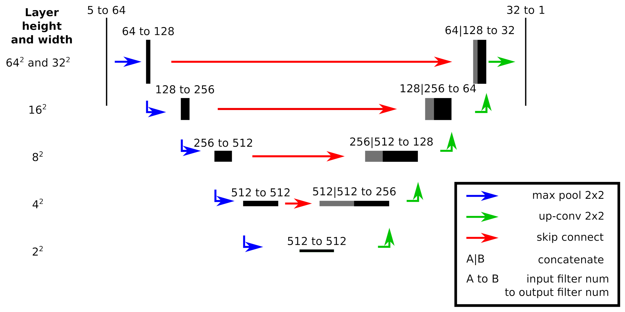
2.1. Model
2.2. Data Source
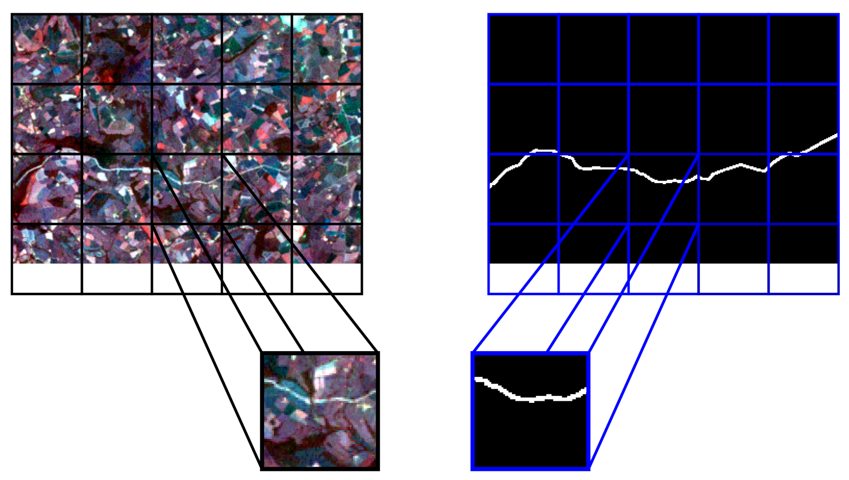
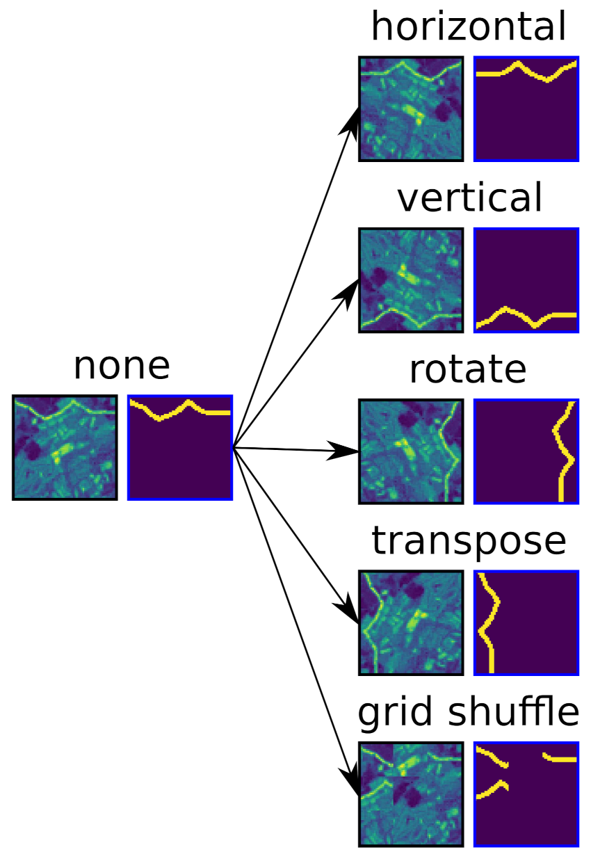
2.3. Image Data Processing
2.4. Training and Validation Process
3. Results and Discussion
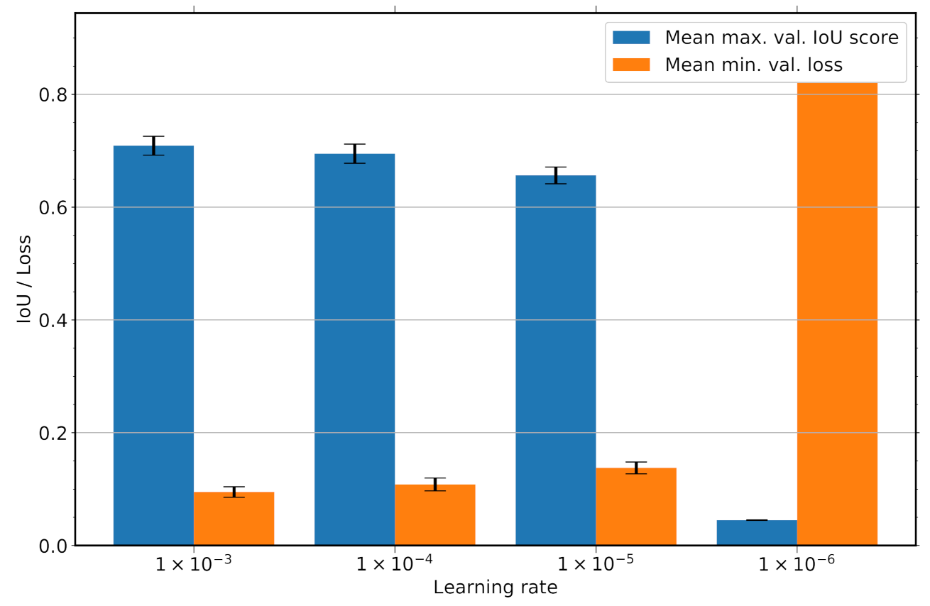
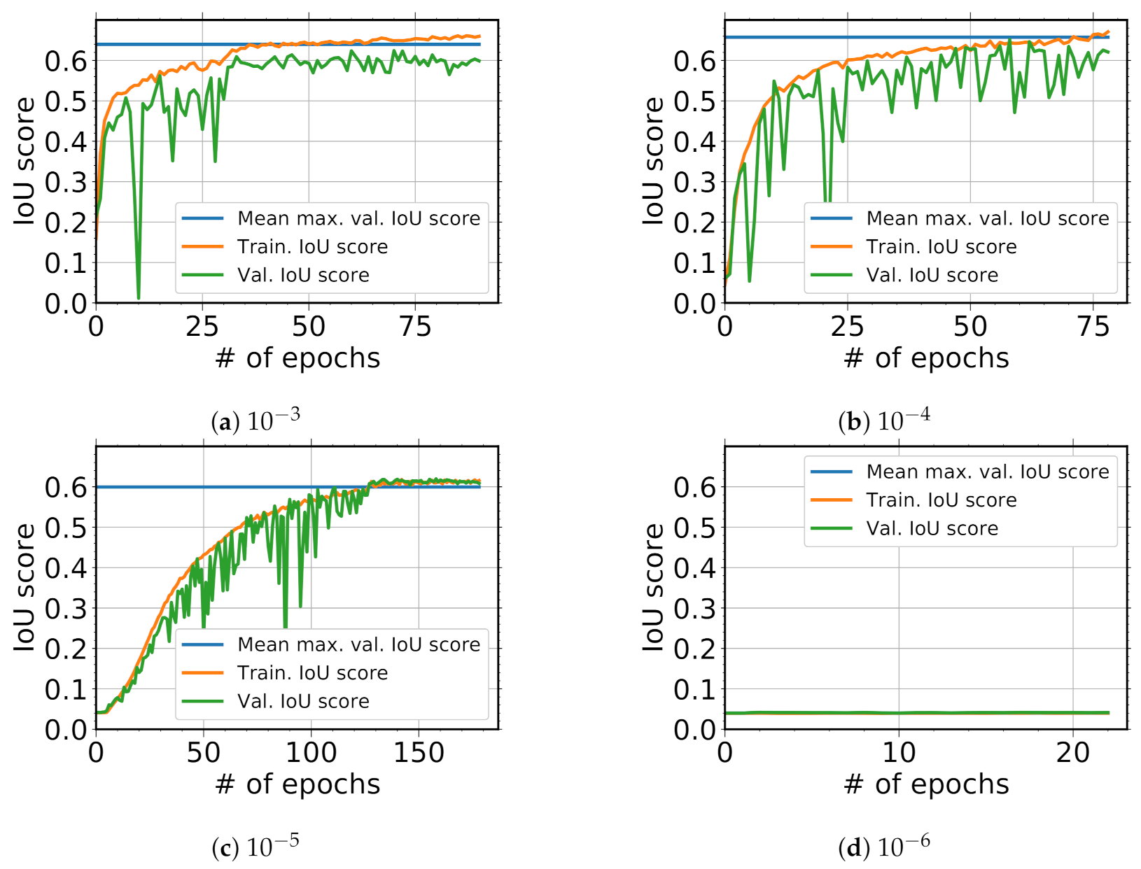
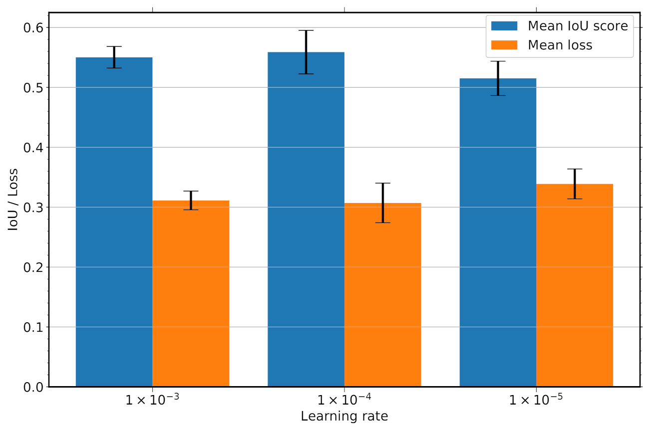
3.1. Training and Validation
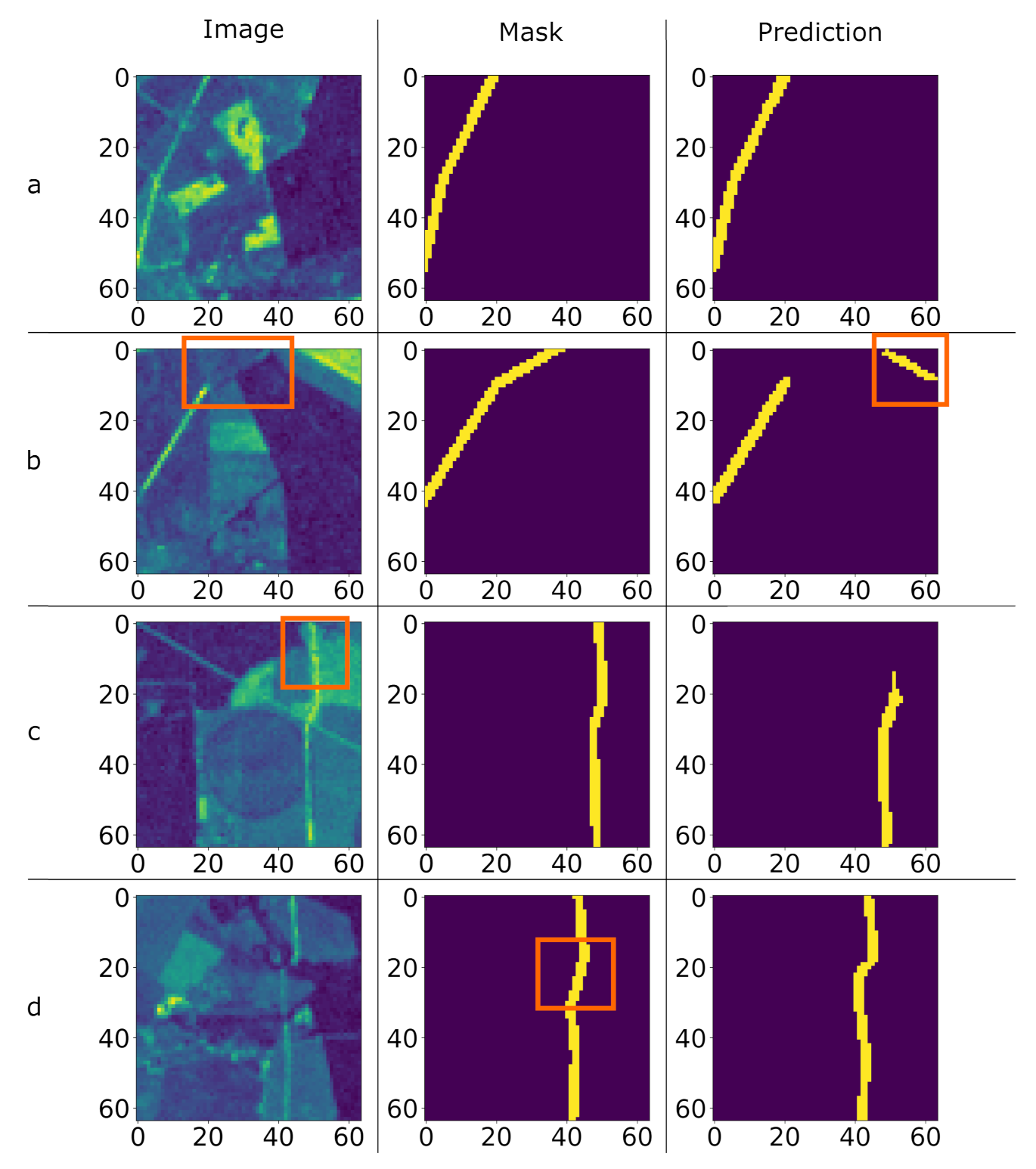
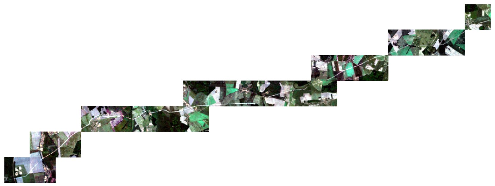
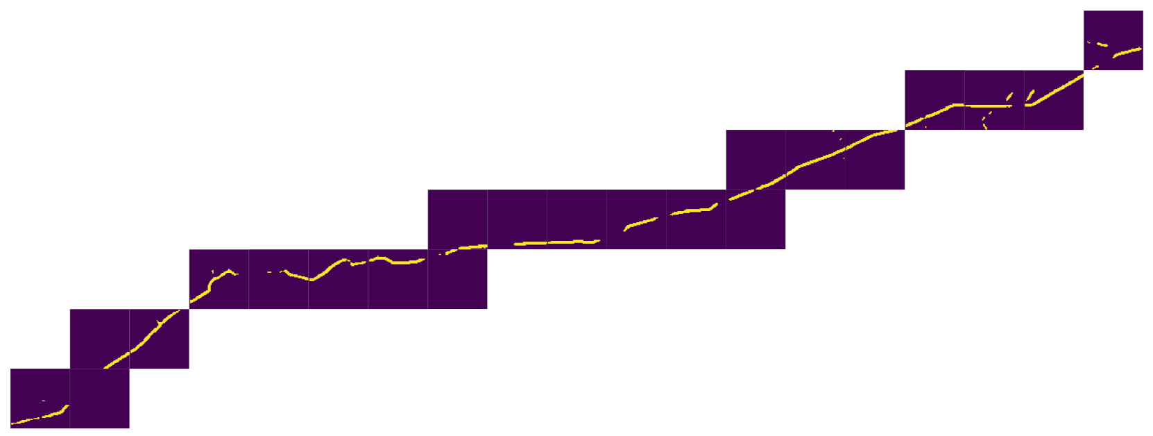
3.2. Testing
4. Summary
Author Contributions
Funding
Data Availability Statement
Acknowledgments
Conflicts of Interest
References
- Brown, T.; Schlachtberger, D.; Kies, A.; Schramm, S.; Greiner, M. Synergies of sector coupling and transmission reinforcement in a cost-optimised, highly renewable European energy system. Energy 2018, 160, 720–739. [Google Scholar] [CrossRef] [Green Version]
- Qadrdan, M.; Abeysekera, M.; Chaudry, M.; Wu, J.; Jenkins, N. Role of power-to-gas in an integrated gas and electricity system in Great Britain. Int. J. Hydrogen Energy 2015, 40, 5763–5775. [Google Scholar] [CrossRef]
- Clegg, S.; Mancarella, P. Integrated Modeling and Assessment of the Operational Impact of Power-to-Gas (P2G) on Electrical and Gas Transmission Networks. IEEE Trans. Sustain. Energy 2015, 6, 1234–1244. [Google Scholar] [CrossRef]
- Clegg, S. Storing renewables in the gas network: Modelling of power-to-gas seasonal storage flexibility in low-carbon power systems. Iet Gener. Transm. Distrib. 2016, 10, 566–575. [Google Scholar] [CrossRef]
- Medjroubi, W.; Müller, U.P.; Scharf, M.; Matke, C.; Kleinhans, D. Open data in power grid modelling: New approaches towards transparent grid models. Energy Rep. 2017, 3, 14–21. [Google Scholar] [CrossRef]
- Matke, C.; Medjroubi, W.; Kleinhans, D.; Sager, S. Structure analysis of the German transmission network using the open source model SciGRID. In Advances in Energy System Optimization; Springer: Berlin/Heidelberg, Germany, 2017; pp. 177–188. [Google Scholar]
- Pluta, A.; Lünsdorf, O. esy-osmfilter: A Python Library to Efficiently Extract OpenStreetMap Data. J. Open Res. Softw. 2020, 8, 19. [Google Scholar] [CrossRef]
- Kunz, F.; Kendziorski, M.; Schill, W.P.; Weibezahn, J.; Zepter, J.; von Hirschhausen, C.R.; Hauser, P.; Zech, M.; Möst, D.; Heidari, S.; et al. Electricity, Heat, and Gas Sector Data for Modeling the German System; Technical Report, DIW Data Documentation; EconStor: Berlin, Germany, 2017. [Google Scholar]
- Schmidt, M.; Aßmann, D.; Burlacu, R.; Humpola, J.; Joormann, I.; Kanelakis, N.; Koch, T.; Oucherif, D.; Pfetsch, M.E.; Schewe, L.; et al. Gaslib—A library of gas network instances. Data 2017, 2, 40. [Google Scholar] [CrossRef] [Green Version]
- Van der Werff, H.; Van der Meijde, M.; Jansma, F.; Van der Meer, F.; Groothuis, G.J. A spatial-spectral approach for visualization of vegetation stress resulting from pipeline leakage. Sensors 2008, 8, 3733–3743. [Google Scholar] [CrossRef] [PubMed] [Green Version]
- Zakharov, I.; Adlakha, P.; Puestow, T.; Power, D.; Warren, S.; Howell, M. Monitoring Pipeline Right of Way Using Optical Satellite Imagery. In Proceedings of the 11th Pipeline Technology Conference, Berlin, Germany, 23–25 May 2016. [Google Scholar]
- Tran, L.A.; Le, M.H. Robust U-Net-based road lane markings detection for autonomous driving. In Proceedings of the 2019 International Conference on System Science and Engineering (ICSSE), Dong Hoi City, Vietnam, 20–21 July 2019; IEEE: New York, NY, USA, 2019; pp. 62–66. [Google Scholar]
- Wei, Y.; Zhang, K.; Ji, S. Road Network Extraction from Satellite Images Using CNN Based Segmentation and Tracing. In Proceedings of the IGARSS 2019-2019 IEEE International Geoscience and Remote Sensing Symposium, Yokohama, Japan, 28 July–2 August 2019; IEEE: New York, NY, USA, 2019; pp. 3923–3926. [Google Scholar]
- Dasenbrock, J. Pipeline Detection with Satellite Images Using Machine Learning. Master’s Thesis, University of Oldenburg, Oldenburg, Germany, 2020. [Google Scholar]
- LeCun, Y.; Bengio, Y.; Hinton, G. Deep learning. Nature 2015, 521, 436–444. [Google Scholar] [CrossRef]
- Yuan, X.; Ou, C.; Wang, Y.; Yang, C.; Gui, W. A layer-wise data augmentation strategy for deep learning networks and its soft sensor application in an industrial hydrocracking process. IEEE Trans. Neural Netw. Learn. Syst. 2019, 32, 3296–3305. [Google Scholar] [CrossRef] [PubMed]
- Yuan, X.; Li, L.; Shardt, Y.A.; Wang, Y.; Yang, C. Deep learning with spatiotemporal attention-based LSTM for industrial soft sensor model development. IEEE Trans. Ind. Electron. 2020, 68, 4404–4414. [Google Scholar] [CrossRef]
- Ching, T.; Himmelstein, D.S.; Beaulieu-Jones, B.K.; Kalinin, A.A.; Do, B.T.; Way, G.P.; Ferrero, E.; Agapow, P.M.; Zietz, M.; Hoffman, M.M.; et al. Opportunities and obstacles for deep learning in biology and medicine. J. R. Soc. Interface 2018, 15, 20170387. [Google Scholar] [CrossRef] [Green Version]
- Wurm, M.; Droin, A.; Stark, T.; Geiß, C.; Sulzer, W.; Taubenböck, H. Deep learning-based generation of building stock data from remote sensing for urban heat demand modeling. Isprs Int. J. Geo-Inf. 2021, 10, 23. [Google Scholar] [CrossRef]
- Knopp, L.; Wieland, M.; Rättich, M.; Martinis, S. A deep learning approach for burned area segmentation with Sentinel-2 data. Remote Sens. 2020, 12, 2422. [Google Scholar] [CrossRef]
- Voulodimos, A.; Doulamis, N.; Doulamis, A.; Protopapadakis, E. Deep learning for computer vision: A brief review. Comput. Intell. Neurosci. 2018, 2018, 8349. [Google Scholar] [CrossRef] [PubMed]
- Guo, Y.; Liu, Y.; Georgiou, T.; Lew, M.S. A review of semantic segmentation using deep neural networks. Int. J. Multimed. Inf. Retr. 2018, 7, 87–93. [Google Scholar] [CrossRef] [Green Version]
- University of Freiburg. Our U-Net Wins Two Challenges at ISBI 2015. Available online: https://lmb.informatik.uni-freiburg.de/people/ronneber/isbi2015/ (accessed on 12 October 2020).
- Goceri, E. Challenges and recent solutions for image segmentation in the era of deep learning. In Proceedings of the 2019 Ninth International Conference on Image Processing Theory, Tools and Applications (IPTA), Ataşehir/İstanbul, Turkey, 7–9 November 2019; IEEE: New York, NY, USA, 2019; pp. 1–6. [Google Scholar]
- Ronneberger, O.; Fischer, P.; Brox, T. U-net: Convolutional networks for biomedical image segmentation. In Proceedings of the International Conference on Medical Image Computing and Computer-Assisted Intervention, Munich, Germany, 5–9 October 2015; Springer: Berlin/Heidelberg, Germany, 2015; pp. 234–241. [Google Scholar]
- Zech, M.; Ranalli, J. Predicting PV Areas in Aerial Images with Deep Learning. In Proceedings of the 2020 47th IEEE Photovoltaic Specialists Conference (PVSC), Online, 15 June–21 August 2020; IEEE: New York, NY, USA, 2020; pp. 767–774. [Google Scholar]
- Çiçek, Ö.; Abdulkadir, A.; Lienkamp, S.S.; Brox, T.; Ronneberger, O. 3D U-Net: Learning dense volumetric segmentation from sparse annotation. In Proceedings of the International Conference on Medical Image Computing and Computer-Assisted Intervention, Athens, Greece, 17–21 October 2016; Springer: Berlin/Heidelberg, Germany, 2016; pp. 424–432. [Google Scholar]
- Islam, M.; Vibashan, V.S.; Jose, V.J.M.; Wijethilake, N.; Utkarsh, U.; Ren, H. Brain Tumor Segmentation and Survival Prediction Using 3D Attention UNet. In Brainlesion: Glioma, Multiple Sclerosis, Stroke and Traumatic Brain Injuries; Crimi, A., Bakas, S., Eds.; Springer International Publishing: Cham, Switzerland, 2020; pp. 262–272. [Google Scholar]
- Frajberg, D.; Fraternali, P.; Torres, R.N. Convolutional neural network for pixel-wise skyline detection. In Proceedings of the International Conference on Artificial Neural Networks, Alghero, Italy, 11–14 September 2017; Springer: Berlin/Heidelberg, Germany, 2017; pp. 12–20. [Google Scholar]
- Bai, Y.; Mas, E.; Koshimura, S. Towards operational satellite-based damage-mapping using u-net convolutional network: A case study of 2011 tohoku earthquake-tsunami. Remote Sens. 2018, 10, 1626. [Google Scholar] [CrossRef] [Green Version]
- Zhang, Z.; Liu, Q.; Wang, Y. Road extraction by deep residual u-net. IEEE Geosci. Remote Sens. Lett. 2018, 15, 749–753. [Google Scholar] [CrossRef] [Green Version]
- Yakubovskiy, P. Segmentation Models. Available online: https://github.com/qubvel/segmentation_models (accessed on 20 November 2019).
- Global Energy Monitor. National Transmission System. Available online: https://www.gem.wiki/National_Transmission_System (accessed on 16 September 2020).
- Kennedy, J.L. Oil and Gas Pipeline Fundamentals; Pennwell Corp.: Tulsa, OK, USA, 1984. [Google Scholar]
- National Grid UK. Network Route Maps. Available online: https://www.nationalgrid.com/uk/gas-transmission/land-and-assets/network-route-maps (accessed on 10 September 2020).
- Europipe. Referenzprojekte. Available online: https://www.europipe.com/de/referenzen/referenzprojekte#c1538 (accessed on 3 February 2020).
- Gillies, S. Shapely: Manipulation and Analysis of Geometric Objects. Available online: https://github.com/Toblerity/Shapely (accessed on 10 May 2020).
- Sayler, K.; Zanter, K. Landsat 4-7 Collection 1 (C1) Surface Reflectance (LEDAPS) Product Guide; USGS: Reston, VA, USA, 2020. [Google Scholar]
- Greff, K.; Srivastava, R.K.; Koutník, J.; Steunebrink, B.R.; Schmidhuber, J. LSTM: A search space odyssey. IEEE Trans. Neural Netw. Learn. Syst. 2016, 28, 2222–2232. [Google Scholar] [CrossRef] [PubMed] [Green Version]
- Goodfellow, I.; Bengio, Y.; Courville, A. Deep Learning; MIT Press: Cambridge, MA, USA, 2016; Chapter 11; Available online: http://www.deeplearningbook.org (accessed on 8 August 2021).
- Bishop, C.M. Pattern Recognition and Machine Learning; Springer: Berlin/Heidelberg, Germany, 2006; Chapter 1. [Google Scholar]
- Murphy, K.P. Machine Learning: A Probabilistic Perspective; MIT Press: Cambridge, MA, USA, 2012. [Google Scholar]
- Sudre, C.H.; Li, W.; Vercauteren, T.; Ourselin, S.; Cardoso, M.J. Generalised dice overlap as a deep learning loss function for highly unbalanced segmentations. In Deep Learning in Medical Image Analysis and Multimodal Learning for Clinical Decision Support; Springer: Berlin/Heidelberg, Germany, 2017; pp. 240–248. [Google Scholar]
- Jadon, S. A survey of loss functions for semantic segmentation. In Proceedings of the 2020 IEEE Conference on Computational Intelligence in Bioinformatics and Computational Biology (CIBCB), Online, 27–29 October 2020; IEEE: New York, NY, USA, 2020; pp. 1–7. [Google Scholar]
- Kingma, D.P.; Ba, J. Adam: A method for stochastic optimization. arXiv 2014, arXiv:1412.6980. [Google Scholar]
- Ulku, I.; Akagunduz, E. A survey on deep learning-based architectures for semantic segmentation on 2d images. arXiv 2019, arXiv:1912.10230. [Google Scholar]
- Géron, A. Hands-On Machine Learning with Scikit-Learn, Keras, and Tensorflow: Concepts, Tools, and Techniques to Build Intelligent Systems; O’Reilly Media: Sebastopol, CA, USA, 2019; Chapter 4. [Google Scholar]
- Mnih, V. Machine Learning for Aerial Image Labeling. Ph.D. Thesis, University of Toronto, Toronto, ON, Canada, 2013. [Google Scholar]


Publisher’s Note: MDPI stays neutral with regard to jurisdictional claims in published maps and institutional affiliations. |
© 2021 by the authors. Licensee MDPI, Basel, Switzerland. This article is an open access article distributed under the terms and conditions of the Creative Commons Attribution (CC BY) license (https://creativecommons.org/licenses/by/4.0/).
Share and Cite
Dasenbrock, J.; Pluta, A.; Zech, M.; Medjroubi, W. Detecting Pipeline Pathways in Landsat 5 Satellite Images with Deep Learning. Energies 2021, 14, 5642. https://doi.org/10.3390/en14185642
Dasenbrock J, Pluta A, Zech M, Medjroubi W. Detecting Pipeline Pathways in Landsat 5 Satellite Images with Deep Learning. Energies. 2021; 14(18):5642. https://doi.org/10.3390/en14185642
Chicago/Turabian StyleDasenbrock, Jan, Adam Pluta, Matthias Zech, and Wided Medjroubi. 2021. "Detecting Pipeline Pathways in Landsat 5 Satellite Images with Deep Learning" Energies 14, no. 18: 5642. https://doi.org/10.3390/en14185642