Article

Towards Understanding the Structure of Subcritical and Transcritical Liquid–Gas Interfaces Using a Tabulated Real Fluid Modeling Approach

IFP Energies Nouvelles, 1 et 4 Avenue de Bois-Préau, 92852 Rueil-Malmaison, France
*
Authors to whom correspondence should be addressed.
Energies 2021, 14(18), 5621; https://doi.org/10.3390/en14185621
Submission received: 28 June 2021 / Revised: 23 August 2021 / Accepted: 25 August 2021 / Published: 7 September 2021

Abstract

:
A fundamental understanding and simulation of fuel atomization, phase transition, and mixing are among the topics researchers have struggled with for decades. One of the reasons for this is that the accurate, robust, and efficient simulation of fuel jets remains a challenge. In this paper, a tabulated multi-component real-fluid model (RFM) is proposed to overcome most of the limitations and to make real-fluid simulations affordable. Essentially, a fully compressible two-phase flow and a diffuse interface approach are used for the RFM model, which were implemented in the CONVERGE solver. PISO and SIMPLE numerical schemes were modified to account for a highly coupled real-fluid tabulation approach. These new RFM model and numerical schemes were applied to the simulation of different fundamental 1-D, 2-D, and 3-D test cases to better understand the structure of subcritical and transcritical liquid–gas interfaces and to reveal the hydro-thermodynamic characteristics of multicomponent jet mixing. The simulation of a classical cryogenic injection of liquid nitrogen coaxially with a hot hydrogen jet is performed using thermodynamic tables generated by two different equations of state: Peng–Robinson (PR) and Soave–Redlich–Kwong (SRK). The numerical results are finally compared with available experimental data and published numerical studies with satisfactory agreement.

Graphical Abstract

1. Introduction

More efficient and cleaner engines is one of today’s highly debated topics in various research laboratories and industries. In modern combustion engines, such as cryogenic engines, gas turbines, and high-pressure diesel engines, this target can be met by increasing the operating injection and ambient pressures up to supercritical conditions. Generally, when a fuel at subcritical temperature and supercritical pressure is injected into a high pressure-temperature environment above the fuel’s critical point, the fuel jet mixes with the chamber gas past its critical temperature.
This class of two-phase flows is known as transcritical injection [1,2,3,4,5,6,7,8,9,10,11,12,13]. A fundamental understanding and simulation of such transcritical flows are among the topics researchers have been struggling with for decades. One of the reasons for this is that the accurate, robust, and efficient simulation of fuel jets remains a real challenge. In this paper, a tabulated multi-component real-fluid model (RFM) is proposed to overcome most of the limitations.

1.1. Review on Supercritical Fluids and Transcritical Injection

Interest in the behavior of supercritical fluids is not new, dating back to at least 1869 [13]. Over the past few decades, researchers have conducted several studies to better understand the dynamics of multiphase flows in this regime [5,6,8,9,10,11,12,14,15,16].
The traditional perspective regarding supercritical fluid behavior was that the distinction between the liquid and gas phases vanishes above the critical point, and a single phase fluid replaces the two-phase system of the subcritical condition. Nevertheless, the supercritical fluid was already known to have properties close to a gas (gas-like) at high temperature ( T > T c ), and properties close to a liquid (liquid-like) at low temperature. The boundary separating liquid-like and gas-like when the fluid temperature is increased has been the focus of recent investigations (see [5,6,11]).
Indeed, for a single-component fluid, it is revealed that these two regions could be separated by a virtual line, the so-called Widom line or pseudo-boiling line [5,6,11]. This line is the extension of the coexisting line in subcritical conditions (see Figure 1d), so that the thermodynamic and transport properties around this line are very sensitive to the variation of temperature ( T ) , pressure ( P ) , and mass fraction ( Y m ) , where m is the component index in the case of a multi-component fluid mixture.
Hence, a slight variation in ( T ) , ( P ) , or ( Y m ) leads to a highly non-linear variation in the properties values, especially close to the critical point, as depicted in Figure 1 for the density and heat capacity of nitrogen as an example. It is well known that fuels have various special features in the supercritical regime, and great efforts have been made to better understand this regime. Several attempts have been made to find unifying concepts for explaining the behavior of fuels in different regimes, and transition from one phase to another.
There are different criteria for distinguishing the liquid-like and gas-like regions based on the isobaric heat capacity C P , isothermal compressibility K T , or thermal expansion coefficient α P [17,18]. Gallo et al. [17] derived, based on experiments and simulations, the lines of the maxima of C P , K T , and α P above the critical point of pure water, and they found that the C P and α P maxima follow a similar path, while the maxima of K T deviate from that of C P and α P for high temperatures.
Banuti et al. [6] determined a simple algebraic expression with a good accuracy for the Widom-line in terms of reduced pressure and reduced temperature, which allows for a simple determination of the positions of maxima in thermal expansion and heat capacity.
Hence, as a unified parameter for detecting the liquid-like and gas-like from each other, the studies showed that the maximum of heat capacity can be a good candidate to identify the interface between phases [5,8]. It is interesting to mention that, based on the idea of maximum of heat capacity and the work of Michelsen [19], Yang et al. [8,9] proposed a criterion for distinguishing between liquid-like and gas-like in the supercritical regime so that the fluid is considered as liquid-like when the compressibility factor is less than 3.5 b P R T , where b is the co-volume given in Table 1.
Based on the experimental study of Chehroudi et al. [2], Figure 1 shows the behavior of the pure nitrogen jet in subcritical ( a ) , transcritical ( b ) , and supercritical ( c ) conditions. The liquid nitrogen jet with different temperatures, varying from 99 to 110 K, was injected into supercritical nitrogen with a fixed temperature of 300 K, T c = 126.2 K. The chamber pressure for this study varies from subcritical values to supercritical ones, approximately from 3 MPa to 9 MPa, P c = 3.396 MPa. It can be seen that, starting from a subcritical pressure condition, an isobaric path crosses the saturation line (see Figure 1d).
In addition, due to the significant surface tension, the interface between the liquid and the gas plays an important role, and this leads to the appearance of primary and secondary breakup, known as classical atomization (see Figure 1a). However, as the pressure increases, the magnitude of the surface tension decreases and vanishes at the critical point, which suppresses the formation of ligaments and droplets, as demonstrated in Figure 1b,c. However, liquid-like ligaments (called also finger-like) can be seen in Figure 1b despite the absence of surface tension.
In addition, the behavior of different nitrogen properties, such as the density and isobaric heat capacity at a transcritical regime (at 4 MPa), are plotted in Figure 1e using the Peng–Robinson equation of state. As shown in this figure, highly thermodynamic non-linearity can be observed around the Widom line (see Figure 1e). The region before the maximum of heat capacity with a similar density value as liquids is called the liquid-like region, and the region after this peak with a density similar to a gas one is called the gas-like region.
The pseudo-boiling transition region (bounded in Figure 1d by the dashed lines around the Widom line) becomes larger as the pressure increases, inducing weaker transcritical non-linearity of the properties. This transcritical behavior has been extensively studied theoretically, experimentally, and numerically by various researchers for single components [2,3,11,16]. In the recent decade, different studies have been done for multi-component fluids, and a similar transition behavior as for pure components has been reported [4,8,9,10,11,12].
However, the transition from subcritical to supercritical regimes does not rigorously follow the transition for a single-component fuel, and the interface structure and evolution in transcritical condition is still not well understood. Indeed, various experimental and numerical studies, such as molecular dynamics simulations as well as CFD simulations have been performed, and they proposed different approaches for introducing a universal criterion for this transition by defining some dimensionless parameters [4,10,20].
Crua et al. [4] studied the injection of n-heptane, n-dodecane, and n-hexadecane into the ambient gaseous nitrogen at different temperatures and pressures. They investigated the transition from subcritical to the diffuse mixing regime as a function of the pure fuels’ critical temperature and pressure. However, due to the limited accuracy of the experimental setup, reliable data are still lacking for the validation of numerical models, and there are still multiple doubts and questions about the conditions and mechanisms behind the interface disappearance for multi-component systems.
Yang et al. [9] suggested that the transition from subcritical to the diffusive mixing regime happens at the critical point of the mixture and especially at pressures higher than the mixture critical pressure. However, this pressure is not constant and depends on the mixture composition.
Ayyappan et al. [20] used a high-speed imaging technique to understand the jet behavior of mixture of fluoroketone- N 2 . They showed that the composition of fluid in the chamber environment plays a critical role in altering the jet behavior, and that the thermodynamic transition of the liquid jet depends upon the injection Reynolds number and chamber pressure for a single component system. However, in a binary system, the transition depends, only and heavily, on the partial pressure of the respective components in the chamber environment. When the chamber environment was pure nitrogen in their study, the jet exhibited the Rayleigh mode of instability. As the amount of fluoroketone was increased in the ambient environment (a binary mixture), the atomization regime changed from the Rayleigh regime to the Taylor regime.

1.2. Review on Numerical and Thermodynamic Models for Two-Phase Flows

From the numerical perspective, several numerical schemes have been proposed in the literature in the past decades for the numerical simulation of two phase flows in which the interface computation is a critical component [8,9,21,22]. Mainly, two types of methodologies have been adopted, namely interface tracking and interface capturing methods [21,22,23,24,25,26,27,28,29,30,31,32].
On the one hand, in the interface tracking method, the interface is tracked by the motion of particles on the interface, and a special modeling for capturing the interfacial dynamics is required. On the other hand, in the interface capturing method, the interface is captured implicitly in each cell of the computational grid with an additional scalar.
Three main methods have been proposed in this class as
  • Volume of Fluid method ( V O F ) , see for instance [26,27,28,29].
  • Level Set Method ( L S M ) , see for instance [33,34,35].
  • Diffuse Interface Method ( D I M ) , see for instance [22,23,24,32].
Generally, the simulation of single-phase compressible flows is known to be challenging, mainly because of the possible appearance of shock waves. However, additional difficulties may appear for two-phase flow solvers due to the abrupt variation of thermodynamic properties across the subcritical interface and also across the Widom line, which may be considered as a transcritical interface. From a numerical point of view, the non-linearity of the thermodynamic properties (due to evaporation, boiling, flash-boiling in subcritical regime, and pseudo-boiling in the transcritical regime) makes the numerical simulation more severe and difficult.
As a consequence, spurious pressure oscillations may appear in such multi-phase flow simulations. However, it was demonstrated by Yi et al. [8] that these spurious oscillations may be tackled when a sufficiently refined grid is employed. Another important issue is related to the fact that the liquid–gas interface disappears during the transition of the fluid to the supercritical state. However, this could also re-appear when a second and different species is injected near a transcritical interface, as shown in Figure 2a.
This interface appearance and vanishing phenomena may occur at any location of the liquid bulk surface. This important flow characteristic explains why cryogenic injection simulations require real fluid models, such as the one proposed in this work, and are usually performed using a Diffuse interface method ( D I M ) , because they are difficult to perform using interface capturing with numerical reconstruction methods, such as V O F [35] and/or L S M [21].
Indeed, the idea of adopting the DIM approach seems appropriate for the simulation of the transcritical regime as the liquid-like and the gas-like are separated by a much thicker interface than in sub-critical conditions. A similar approach is also applied for the premixed combustion modeling with a thickened flame model ( T F M ) [36] designed for increasing the flame thickness in the LES framework.
Another advantage of the DIM method is that explicitly satisfying the interface conditions is not required, and the variation of the interface topology is automatically handled, which is computationally efficient. However, the diffused interface have to be maintained relatively sharp in subcritical conditions and specific sub-grid scale modeling for high frequency interface instability, and breakup is required in order to properly simulate the liquid jet primary atomization [37].
In the DIM framework, many two-phase flow models have been developed in the literature with the number of transport equations ranging from three to seven based on the initial equilibrium assumptions, and it has been proven that the robustness of these models is completely coupled with the resolving of large density gradients due to the transition from the liquid to the gas. A comprehensive review of different models for DIM can be found in [22].
As a result, the prediction of the thermodynamic and transport properties of transcritical two-phase flows using the DIM approach will be of importance, and employing an appropriate equation of state will be crucial. Indeed, as proven by extensive studies, the ideal gas equation of state ( E o S ) is no longer valid at transcritical conditions. Figure 3 proves that, due to the importance of density, heat capacity, and other thermodynamic properties, a more general and accurate real fluid EoS is required for studying the two-phase flows in this regime.
As Figure 3 shows, using different EoS results in various predictions for different properties. Figure 3a–d demonstrate the density, heat capacity, sound speed, and viscosity profiles for pure nitrogen using different EoS, such as ideal gas, PR (Peng Robinson), and SRK (Soave–Redlich–Kwong). As can be seen in this figure, compared to the NIST data [38], the ideal gas EoS cannot predict the transcritical behavior of properties at this regime, and using more complex EoS is mandatory for accurate studies.
Moreover, as shown in Figure 3a, the SRK-EoS can predict the nitrogen density much better than the PR-EoS when compared to the NIST data [38]. These results corroborate many published ones. Indeed, previous studies have performed various and more comprehensive studies on the accuracy of different EoS, and it has been reported that, generally, for cryogenic conditions, the SRK-EoS gives the best prediction of the fluid density [39]. Generally, PR is better for heavy fuels; however, SRK is better for light fuels (gases) [12]. Therefore, both SRK and PR will be tested in this work to corroborate previous works.

1.3. Subcritical, Transcritical, and Supercritical Real Fluid Mixing Injection

In recent years, researchers have performed different studies for multi-component systems to have a clearer picture of the mixing jet behavior for multi-component systems, without considering the complexities of combustion, known as cold flow studies [9,11,30,40,41,42]. In this paper, different studies will be carried out for pure single-component as well as for binary mixtures to better understand and highlight the main difference between them, and to investigate the phase transition and mixing processes in subcritical, transcritical, and supercritical regimes. Among them, one of the fundamental studies could be the study of cryogenic nitrogen ( N 2 ) injected co-axially with warm hydrogen ( H 2 ) into supercritical nitrogen ambient [41,43].
Figure 2a represents a schematic of such a cryogenic injection flow close to the mixing injector orifice. As can be seen, there are two different propellant streams ( N 2 and H 2 ), called the main stream and secondary stream, respectively. The mainstream cryogenic liquid L N 2 with the temperature of 118 K at the subcritical temperature regime (as T c = 126.2 K, and P c = 3.396 MPa of N 2 ), is injected co-axially with a warm secondary stream of gaseous G H 2 with the temperature of 270 K, ( U N 2 i n j = 5 m/s) ( < U H 2 i n j = 120 m/s). These streams are injected into a chamber filled with gaseous G N 2 at T C h = 300 K, and P C h = 4 MPa, and hence at supercritical condition.The configuration sketched in Figure 2a is intended to summarize the discussion throughout this paper by showing the main characteristics of the flow field with a transcritical and subcritical interface simultaneously. Since a large number of thermodynamic and physical parameters are involved in this problem, it cannot be treated in a single study.
Figure 2. (a) Schematic for a liquid-like L N 2 main stream injected in the center, and a secondary hot supercritical gaseous H 2 injected co-axially into a combustor at a pressure higher than the critical pressures of the two non premixed components. This figure sketches the case in which the liquid core is partially covered by G H 2 jet. The liquid core interface is divided into two parts. The leading interface part 1 is a transcritical interface (see the dashed line colored in red). A subcritical interface is formed upstream between the main L N 2 flow and the secondary G H 2 flow (see the dashed line colored in blue). (b) The gas volume fraction contour plot in a temperature and H 2 composition diagram shows the locus and the thermodynamic states for subcritical ( N 2 - H 2 ) interface. (c) The isobaric heat capacity of N 2 , has a peak value, on the Widom line, at the transcritical interface between L N 2 and G N 2 .
Energies 14 05621 g002
The current work focuses on studying the phase transition characteristics in order to reveal the parameters with the dominant roles. As shown in Figure 2a, the main L N 2 flow field immediately downstream of the injector orifice is heated and forms a thermal mixing layer between the propellant jets and chamber gas, here between the liquid-like nitrogen and supercritical fluids. From a thermodynamic viewpoint, as previously discussed, one of the main characteristics for the transcritical interface is the appearance of extrema for the heat capacity at the Widom line, as shown in Figure 2c and Figure 3b.
However, due to the different velocities of the propellant between the main flow L N 2 and the secondary flow G H 2 , the composition may vary significantly depending on the position, and, as a consequence, the fluid properties vary accordingly. Indeed, the G H 2 jet can cover entirely or not the L N 2 jet liquid core. The mixture critical point will change as soon as the composition changes in the multicomponent mixtures, and a linear relation between the critical point of a mixture and that of each pure species does not exist.
Hence, the bubble line and dew line locus will be shifted in proportion to the composition value. Figure 4 also shows the phase boundary movements as well as critical point variations for different compositions for the binary mixture of N 2 - H 2 , and this demonstrates that, by the mixing of two supercritical components, it may actually find a subcritical behavior for the mixture. However, due to this fact that the pressure in the chamber approximately remains constant, the critical point as well as the bubble line and dew line locus no longer depend on the mixture composition, as shown in Figure 2b.
Figure 2a sketches the case in which the liquid core is partially covered by the G H 2 jet. In this case, the liquid core interface is divided into two parts. On the one hand, the leading interface part is a transcritical interface where the surface tension is null and only diffusive mixing can take place.
Figure 2c shows the specific heat capacity non-linearity taking place at such a transcritical interface. On the other hand, a subcritical interface is formed upstream between the main L N 2 flow and the secondary G H 2 flow (see Figure 2a). For such a subcritical interface, primary atomization may occur depending on the magnitude of the surface tension.
The path followed by the fluid close to the interface can be sketched by the dotted line in Figure 2b. This figure shows the phase diagram of the H 2 - N 2 mixture at the system pressure of 4 MPa. At the left of the figure, the injected liquid-like N 2 has a temperature of 118 K. When the fluid moves to the right, it is progressively mixed with H 2 at 270 K. The temperature of the jet could be increased in an adiabatic manner by neglecting the heat exchange. This means that it has the temperature such that the enthalpy of the mixture is equal to the weighted average of the enthalpies of the pure jets. In other words ( H ( A M T , P c h ) = z H 2 H H 2 ( T H 2 i n j , P c h ) + ( 1 z H 2 ) H N 2 ( T N 2 i n j , P c h ) ).
The resulting temperature as a function of the fluid composition is shown in Figure 2b. This is called the Adiabatic Mixing Temperature ( A M T ) . The same figure also shows the phase diagram of the mixture: when α g a s = 1 , the fluid behaves as a gas (in the right part, rich in hydrogen). When α g a s = 0 , the fluid behaves as a liquid (on the left part of the diagram. Approximately, between the compositions of 10 to 65 % H 2 , the fluid is in two-phase condition, and this is despite the fact that both of the pure components are supercritical.
In addition, it is also the location of phase change (evaporation or condensation), as the adiabatic mixing temperature ( A M T ) is crossing the two-phase dome, as depicted in Figure 2b. In fact, this subcritical interface is due to the movement of the mixing critical point of the binary ( N 2 , H 2 ).
The gas volume fraction contour plot, at a temperature and H 2 composition diagram is plotted at P = 4 MPa in Figure 2b in order to show the locus and the thermodynamic states for subcritical ( N 2 - H 2 ) interface. By changing the flow rate of the propellants, the position of the transition between the subcritical and the transcritical interfaces changes.
Consequently, this may induce changes in the jet shape, structure, and liquid length, and, as a result, the mixing process. This should affect the interface modeling as discussed above. In addition, the transition from subcritical multi-component interface to transcritical interface will be affected also various other parameters, such as turbulence, the thermal mixing layer, and the hydrodynamic instabilities, such as the Kelvin–Helmholtz instability, by making delay or fasting it, which needs to be further addressed.

1.4. Review on the VLE Tabulation Approach

In order to study the above complex behaviors, employing a real fluid model is mandatory, as explained above. However, real fluid simulations have been proven to be computationally time-consuming, especially for multi-component simulations, including binary mixtures. Indeed, it is found that the complexity of cubic EoS and solving iteratively the Vapor–Liquid–Equilibrium (VLE) using the isoenergetic-isochoric (UV) flash set of equations are computationally expensive [8,9,19,44,45].
Hence, an accurate and, most importantly, robust real-fluid simulation is required, which is one of the main objectives of the presented study. One of the remedies to elevate this problem is setting up a VLE tabulation before the beginning of the simulation and storing the required thermodynamic property values. Then, a rapid searching as well as an interpolation are carried out in this table during the simulations. This process of searching and interpolation is usually called “a look-up table” in the literature.
Indeed, there are previous studies that have proposed various methods for tabulation, interpolation, and look-up of data [46,47,48,49,50,51,52]. Azimian et al. [48] introduced an artificial neural network model for generating the water/steam thermodynamic tables to reduce the computational expenses of solving flash calculations. De Föll et al. [51] proposed a tabulation method based on a projection approach for single-component fluids using a quad-tree data structure.
Lorenzo et al. [49] suggested a 2D single component look-up table method for water-steam simulation. In this work, bilinear functions were used to regularize the shape of the thermodynamic domain in the energy-volume (UV) space, so that an accurate bi-cubic interpolation could be used. Praneeth and Hickey [52] introduced a systematic error quantification and computational cost estimation of EoS for compressible single-component tabulation. They reported that, due to the inherent thermodynamic non-linearity around the pseudo-boiling curve, small errors in the thermodynamic property estimation could lead to large variations in the computed pressure and temperature, which directly affects the thermal and transport properties calculations in the flow.
Most of the above-mentioned studies relating to the tabulated thermodynamic properties focused on single-component fluids. However, few studies have been carried out with multi-component fluid mixture tabulation. One of the notable studies was performed by Brown et al. [47]. They suggested a multi-component two-phase homogeneous equilibrium model (HEM) and flow solver for binary and quaternary mixtures, allowing a two-dimensional (P, T)-based adaptive inverse interpolation approach.
Another notable study was recently conducted by Koukouvinis et al. [45]. In that study, the authors proposed a uniform, tabulated thermodynamic approach based on the NIST-database and VLE using PC-SAFT EoS for simulation of the ECN spray A [45]. They reported that, by using the PC-SAFT EoS and log10(P)-T tabulation approach, the results were independent of table size when bilinear interpolation was adopted, even with linear mixing rules. As a result, to sum up, most of the available studies show that the tabulation should be highly accurate, with low-storage requirements, and a fast lookup algorithm.

1.5. Outline of the Present Study

In this study, a fully compressible multi-component two-phase real fluid model (RFM) [8,9,46] considering vapor liquid equilibrium (VLE) is proposed using a generalized three-dimensional (3D) tabulation method. In this method, an in-house thermodynamic library IFPEN-Carnot is used to generate the 3-D table (with T-P-Y as the axis for a binary mixture) based on various real fluid EoS. This thermodynamic library involves different EoS, such as Peng–Robinson (PR), and Soave–Redlich–Kwong (SRK), which also represents one of its main advantages.
The tabulated thermodynamic properties of the mixture are calculated as a function of the temperature ( T ) , pressure ( P ) , and species composition ( Y ) . The uniform look-up table is generated based on an isothermal-isobaric flash (TPn flash) [53]. This tabulation method also improves the efficiency of the tabulation approach previously developed by Yi et al. [46] based only on the PR-EoS [8,9]. The RFM model along with the generalized 3D tabulation method was implemented in the CONVERGE solver [54].
The present work attempts to investigate the accuracy of the proposed RFM model and the tabulation methodology in conjunction with two different modified numerical schemes, a modified PISO, and a modified SIMPLE algorithms, which were adapted for the real fluid modeling approach. Another objective of this study is to quantify the effects of real fluid thermodynamics on the liquid fuel injection process for pure and multi-component systems in different thermodynamic regimes.
Hence, Section 2 is dedicated to the explanation of the numerical and theoretical methods including the governing equations, thermodynamic tabulation, and look-up methods. Section 3 is devoted to the understanding of transcritical injection by studying some 1-D, 2-D, and 3-D test cases for single components and for multi-component mixtures.
Then, the simulation setup for the cryogenic co-injection of liquid nitrogen ( L N 2 ) and gaseous hydrogen ( G H 2 ) is presented considering two different EoS: PR and SRK. The simulation results are examined and compared with Matheis et al. [40] numerical results and the experimental study of Oschwald et al. [43]. Finally, our conclusions are presented in Section 4.
Figure 3. Comparison and validation of the thermodynamic model calculated in this study with the data of NIST [38] for different EoS for density, isobaric heat capacity, sound speed, and viscosity, respectively, for pure N 2 . PR, and SRK refer to the Peng Robinson, and Soave–Redlich–Kwong equation of states. The viscosity is calculated by the Chung correlation [55].
Energies 14 05621 g003
Figure 4. Phase envelope movements and critical point variations for different compositions for N 2 - H 2 mixture.
Energies 14 05621 g004

2. The Real-Fluid Model (RFM)

As discussed above, many two-phase flow models in the DIM framework have been developed in the literature with the number of transport equations ranging from three to seven based on the initial equilibrium assumptions. In this study, the 4-Equation real fluid (RFM) model developed at IFPEN [8,9,46] is employed assuming the flow system to be under the assumptions of thermodynamic equilibrium (i.e., equilibrium of the velocity, pressure, temperature, and chemical potential at liquid–vapor interfaces). This two-phase flow model is a fully compressible and homogeneous equilibrium model (HEM), which considers multi-component in both phases.
The set of governing equations as employed in the CONVERGE CFD solver [54] was used as a base framework for the development of a modified solver using the tabulated RFM model presented below in this section.

2.1. Governing Equations of the Flow Solver

The set of governing equations are presented through Equations (1)–(4) including the density transport equation, species transport equation, mixture momentum equation, and mixture specific internal energy equation. ( ρ , u i , P , T , e ) are the mixture’s density, velocity, pressure, temperature, and specific internal energy, respectively. ( Y m , h m ) are the mass fraction and enthalpy of species (m), respectively. N s is the total number of species.
ρ t + ρ u i x i = 0
ρ Y m t + ρ Y m u j x j = x j ( ρ D Y m x j ) , m = { 1 N s 1 }
ρ u i t + ρ u i u j x j = P x i + τ i j x j
ρ e t + ρ e u j x j = P u j x j + τ i j u i x j + x j ( λ T x j ) + x j ( ρ D m h m Y m x j )
where the viscous stress tensor ( τ i j ) is given by
τ i j = μ ( u i x j + u j x i ) 2 / 3 μ ( u k x k ) δ i j
The thermal conductivity ( λ ) and the dynamic viscosity ( μ ) cover laminar and turbulent contributions. The laminar contribution of ( λ , μ ) is computed by Chung et al. [55] correlations. The turbulent conductivity is calculated using a given turbulent Prandtl number as ( λ t = C P μ t P r t ) , where ( C p ) is the isobaric heat capacity and the turbulent viscosity ( μ t ) is computed by the adopted turbulence model.
In this work, the standard turbulent subgrid-scale Smagorinsky model is used in the large-eddy simulation (LES) framework [56]. The laminar and turbulent diffusion coefficients are estimated using a given Schmidt number ( S c ) as D = ν / S c , and D t = ν t / S c t , respectively. For high-speed flows that include discontinuity, such as shock-waves, Equation (4) can be employed based on a total energy formulation ( E = e + u 2 i 2 ) as in Equation (6), to ensure energy conservation.
ρ E t + x j ( ρ u j E + u j P u i τ i j λ T x j ) = 0

2.2. Equilibrium Thermodynamic Closure of the Flow Solver, and the Tabulation Look-Up

The fully compressible multi-component two-phase flow system described above is closed by a real-fluid equation of state (EOS), such as the Peng–Robinson (PR) [57], or Soave–Redlich–Kwong (SRK) [58]. More importantly, a thermodynamic equilibrium hypothesis is also adopted to ensure the hyperbolic mathematical formulation of the RFM model.
The current work adopts a tabulation approach where the thermal and transport properties as well as the phase states and compositions are tabulated before the CFD simulation. During the simulation, the various tabulated parameters are robustly interpolated over the entire range of the thermodynamic states based on three inputs for the tables, which are the temperature ( T ) , pressure ( P ) , and species mass fraction ( Y m , m = 1 , N s 1 ), where N s is the total number of species.
The tabulation is carried out based on the IFPEN-Carnot thermodynamic library, which uses a robust isothermal-isobaric (TPn) flash [44] algorithm coupled to various real-fluid equations of state. This (TPn) flash performs the vapor–liquid equilibrium (VLE) calculation, including the thermal, transport properties, and composition in each phase.
This tabulation approach offers the advantage of avoiding the direct evaluation of the non-linear cubic EOS along with the VLE calculation during the simulation, which has been proven to be computationally demanding and costly. Moreover, the tabulation approach based on the IFPEN-Carnot thermodynamic library allows the simulation of different fuels and surrogates without the need of hard coding a (TPn) flash for each EoS of interest.
In addition, the simplistic inverse-distance weighting (IDW) [59] is implemented for the tables interpolation for binary (two-components) mixtures. Hence, the interpolation in the table during the simulation is mainly carried out using two main functions:
  • A Table look-up function:
    Compute the thermal, transport properties as well as the phase state using the input parameters ( T , P , Y m ) .
  • A Reverse look-up function:
    Compute/Update the temperature using the inputs ( e , Y m , P ) .
A general form of finding an interpolated value of u i at a given point X based on samples u i = u ( X i ) , i = 1 , N using IDW can be expressed as Equation (7), where ω i ( X ) = 1 d ( X , X i ) , X denotes an interpolated (arbitrary) point, X i is an interpolating (known) point, d is the given distance from the known point X i to the unknown point X, and N is the total number of known points used in each local interpolation.
u ( X ) = i = 1 n ω i ( X ) u i i = 1 n ω i ( X ) i f d ( X , X i ) 0 for all i u i i f d ( X , X i ) = 0 for some i
A general form of a cubic EoS can be written as Equations (8) and (9) for the SRK and PR EoS, along with the various parameters that are calculated for both equations. The parameters for the two EoS are calculated as listed in Table 1 [57,58].
P = R T ν b a ( T ) ( ν + δ 1 b ) ( ν + δ 2 b )
a i ( T ) = ( a c ) i [ 1 + m i ( 1 T T c ) ] 2
In addition, when the SRK-EoS or the PR-EoS is used for mixtures, Van-der Waals mixing rules are applied as Equation (10) for mixtures, where ( k i j ) is the binary interaction parameter (BIP) that can be fitted to experimental data to well represent the phase diagram of a binary system, x i is the molar fraction, and a i ( T ) is the parameter calculated using Equation (9) for component i. In this study, k i j is set to zero.
a ( T ) = i j x i x j a i ( T ) . a j ( T ) ( 1 k i j ) b = i x i . b i
The procedure of the tabulation using the IFPEN-Carnot thermodynamic library is based on selecting the input parameters ( T , P , Y m ) and the related output properties as ( ρ , e , C p , C v , C s , λ , μ , θ , α , P H I ) . These parameters are stored in the table, as depicted in Figure 5. The computation of the output properties is described in the flowchart, as shown in Figure A1. The grid size in each direction ( T , P , Y m ) will be considered uniform, as shown in Figure 5. The tabulation procedure is summarized with the following steps.
  • Inputs: ( T , P , Y m ) , where ( Y m ) is the initial (feed) mass fraction of species ( m ) and ( m = 1 , N s 1 ) , where ( N s ) is the total number of species.
  • Solve the VLE problem: ( ψ v , x m , y m ) = VLE ( T , P , z m ) , where z m , x m , y m , are species the initial feed (in mole fraction), species molar fraction in the liquid and gas phase, respectively. ψ v is the vapor molar fraction. See [8].
  • If the mixture is in single phase liquid ( ψ v = 0 ) or single phase vapor ( ψ v = 1 ) , then the single phase properties are directly computed. In this configuration, if the density is less than 400 kg/m 3 , then the phase is assumed to be vapor, and if it is greater than 400 kg/m 3 , it is assumed to be liquid.
  • If the mixture is in a two phase state ( 0 < ψ v < 1 ) , compute both the liquid and gas phase properties, then the two-phase mixture properties are evaluated through Equations (A1)–(A7). In (A1)–(A7), α p is the phase volume fraction and ( p = l ; v ) stands for liquid and vapor phases, respectively. The vapor volume fraction is computed from the vapor mole fraction ( ψ v ) as α v = ψ v ν v ψ v ν v + ( 1 ψ v ) ν l . ( ρ , e , C s , m i x ; W o o d ) are the mixture’s density, specific internal energy, and Wood speed of sound.
  • Repeat steps (2 and 3) or (2 and 4), until the specified input ranges for ( T , P , Y m ) are completed for the desired number of points in the table.
Figure 5. Schematic of the thermodynamic table, and the properties calculated, and stored at each cell. P1:P8 are the eight points of the thermodynamic cell surrounding the unknown point (X). The interpolation approach is based on the inverse distance weighting method.
Energies 14 05621 g005

2.3. Validation of the VLE Solver

To validate the VLE thermodynamic solver used in the current study, VLE for H 2 - N 2 using SRK-EoS was compared with the available experimental data [60], as shown in Figure 6. It can be seen that the calculation results are in good agreement with the experimental data over the entire range of pressure for the different temperatures.
Figure 7 shows the variation of different binary mixture properties of H 2 - N 2 as a function of temperature and H 2 mass fraction at P = 4 MPa, including the mixture density, heat capacity, sound speed, and compressibility factor. These results were obtained using a uniform table with Δ T = 1 K, Δ P = 0.1 bar, Δ Y m = 0.005 in grid sizes on the three axis.
By generating an appropriately refined table, some interesting phenomenon, such as the heat capacity ( c p ) peak around the Widom line, can be seen in Figure 7b. In this Figure, it is important to note that this ( c p ) peak exists not only for single component N 2 but also for N 2 - H 2 mixtures, particularly when a small amount of H 2 is mixed with N 2 as long as the mixture remains homogeneous.
As soon as the mixture enters the two-phase zone, the heat capacity has no physical meaning any longer. The plot shows an average value of Cp for the saturated liquid and vapor phases, according to Equation (A4). These figures illustrate the strongly non-linear behavior of these four properties, and therefore the importance of using complex EoS for the regions where the compressibility factor value is far from unity, as shown in Figure 7d.

2.4. Coupling the Flow Solver with the Thermodynamic Solver

The coupling between the flow solver and the thermodynamic solver is one of the critical elements in the RFM model proposed in this article. To our knowledge, most of the available two-phase flow equilibrium solvers in the literature are proposed so that the thermodynamic state in each computational cell will be determined after solving of the mass, momentum, and energy equations [8,9,11,12,30,61].
This means that the flow solver is completely decoupled from the thermodynamic solver, considering the superposition principles. Figure 8a shows a schematic of this typical and conventional approach [9], where the system molar internal energy (U), molar volume (V), and molar numbers (n) are specified, and all other thermal properties are determined using the so called (UVn) flash.
The author’s previous studies demonstrated that, due to the separation of the flow solver and thermodynamic solver, it may lead to the growth of oscillations on the solution fields, which delays the solver’s convergence. More information about this conventional decoupled approach can be found in [8,9]. To dampen the difficulties of multi-phase solvers due to the previous decoupled method, a new and novel algorithm is introduced in this study.
This algorithm is mainly based on the isothermal-isobaric (TPn) flash, which is known to be more robust and efficient. As shown in Figure 8b, a strong coupling between the flow solver and the thermodynamic solver is used throughout the different steps of the SIMPLE numerical scheme. In fact, a similar strong coupling was introduced in the PISO numerical scheme, as depicted in Figure A1. In the following, these two novel iterative algorithms are discussed in the case of the two-phase RFM model:
  • A modified Pressure Implicit with Splitting of Operator (PISO) method of Issa (1986) [62], see Figure A2.
  • A modified Semi-Implicit Method for Pressure-Linked Equations (SIMPLE) method of Patankar, 1980, Figure 8b [63].
The modified SIMPLE algorithm solves the same set of equations as the modified PISO (Equations (1)–(4)). However, they are solved in SIMPLE so that the momentum equation is solved within the iterative algorithm, rather than as a predictor step in PISO.
Generally, it has been accepted that SIMPLE has the advantage of respecting the hyperbolic nature of the transport equations, while using the elliptic nature of the pressure equation. The practical difference between SIMPLE and PISO is that SIMPLE more strongly couples the velocity and the pressure, while it is numerically more expensive than the PISO approach. Using PISO or SIMPLE should finally be decided depending on the nature of the resolved flow.
SIMPLE should be preferred for highly unsteady flows. In order to determine the pressure field, a pressure Poisson equation is derived and solved iteratively using a predictor-corrector PISO or SIMPLE algorithm [54]. Equation (11) is a semi-discretized form of this equation where the superscript n represents the previous field values, and (*) represents the intermediate most up-to-date field values in the iterative algorithm.
ρ t = d t 2 x i x i ( P * P n ) ( ρ n u i * x i )
Considering that Equation (11) is solved in SIMPLE through a double isothermal algorithm as shown in Figure 8b and assuming low variation of the density with the composition, one can write this equation as Equation (12).
ρ β T P t = d t 2 x i x i ( P * P n ) ( ρ n u i * x i )
where β T = 1 ρ ( ρ P ) T is the isothermal compressibility factor. Finally, the fully discretized Poisson equation reads,
2 x i x i ( P * P n ) ( P * P n ) ϕ n d t 2 = ( ρ n u i * x i ) 1 d t
where ϕ n = ( ρ β T ) n , so that
ϕ = ( ρ P ) T = ρ P for ideal gas EoS : P = ρ R T ρ k for barotopic EoS : ρ = ρ 0 e ( P P 0 ) k ρ β T = γ c 2 for real - fluid EoS : ρ = ρ ( P , T , Y m )
The only unknown of Equation (13) is now P * , which can be calculated knowing the first corrector of velocity u i * and the pressure and density values of previous time step, n. After the momentum predictor and first corrector step have been completed, the other transport equations are solved in series. An important point is the calculation of the temperature after solving the energy equation, as shown in Figure 8b at each SIMPLE loop. This temperature calculation is carried out using the reverse look-up function T * = F ( e * , P * , Y m * ) , as explained in Section 2.2. Then, the process of correcting the momentum equation and re-solving is repeated as many times as necessary to achieve the desired accuracy.
To sum up, the implementation of the RFM model can be summarized as follows:
  • Read the thermodynamic table during the simulation setup and initialize the thermal and transport properties as well as the phase state based on the temperature ( T n ) , pressure ( P n ) , and species mass fraction ( Y m n ) in the domain, where the exponent (n) denotes the current time step.
  • Solve the momentum predictor, and then the first corrector step.
  • Solve the transport equations in the order shown in the flow chart, as depicted in Figure 8b.
  • At the end of each iteration loop, the convergence is checked based on the density correction error ρ * ρ n 1 ρ * for density based solver, where ρ * : the current correction for the density, ρ n 1 is the previous value of the density correction, and P * P n 1 P * for pressure based solver, where P * : the current correction for the pressure, and P n 1 is the previous value of the pressure correction. If the specified loop tolerance error is reached, the values of the previous time step are updated before proceeding to the next time step, otherwise a new SIMPLE or PISO loop is performed.
One important subject is related to the density-based solver used in this study to solve the RFM model. Indeed, flow field instabilities may be generated by such a solver when the fluid is almost incompressible and the sound speed is high, so that the Mach number tends to zero. In fact, due to the appearance of liquid as an incompressible fluid, alongside the gas phase as compressible, the simulation of such flows may face numerical difficulties due to large gradients of density, the speed of sound, and the time scale.
As a result, researchers have categorized the problems into compressible and incompressible by introducing density-based and pressure-based solvers. On the one hand, the density-based approach was originally designed for high-speed compressible flows so that the continuity equation is used to obtain the density field, while the pressure field is determined from the equation of state.
The pressure-based solvers, on the other hand, have traditionally been used for incompressible and mildly compressible low mach number flows by manipulating continuity and momentum equations, so that the solution of density transport equation is ignored and the density field is computed via the equations of state. Preliminary studies of the proposed RFM model solver have shown that the instability and the oscillations of the flow field at low pressure cases could be reduced using a pressure-based solver along with some under-relaxation of the pressure ratio.

3. Transcritical Mixing and Evaporation Study

The study of transcritical mixing and evaporation is the main objective of this paper, as discussed before in Figure 2. Hence, a series of different 1-D, 2-D, and 3-D test cases for single component and binary mixture are computed and analyzed for better understanding the mixing of jets involving subcritical and transcritical interfaces.

3.1. 1-D Transcritical Shock Tube Test Cases

In order to validate the RFM model along with the density-based approach proposed above, numerical simulations for different shock tube test cases are carried out as summarized in Table 2. The tube is 1 m long with initial discontinuity at 0.5 m, where the left and right hand side of the tube are initiated as listed in Table 2. The notations L and R in Table 2 stand for the left and right sides of the tube, respectively.
Case 1 represents the simulation of a shock tube for cryogenic N 2 , at supercritical conditions. For these simulations, a first order time accuracy and a second order spatial accuracy are used. For the sake of stability and accuracy, the CFL number is set to 0.1. The results in this study are compared with the study of Ma et al. [11]. These authors developed a fully conservative solver using the PR-EoS without phase change.
Since the pressures and temperatures in both side of shock are above the critical point of nitrogen ( T c N 2 = 126.2 K, P c N 2 = 3.4 MPa), then, the fluid is in a supercritical state. The results of case 1 depicted in Figure 9 show that, compared to Ma et al.’s [11] numerical results, the RFM-SIMPLE has good agreement. However, small differences can be seen in Figure 9 due to the use of the entropy-stable model for damping the spurious oscillations, as discussed in their paper. Such an entropy-stable model has not been considered in the RFM model.
The conformity of the results using different mesh sizes proves the non-grid dependence of the RFM results. As demonstrated in Figure 9e,f showing isobaric heat capacity and the gas volume fraction profiles, respectively, the isobaric heat capacity has its maximum values in the liquid-like region between x = 0.35 m and x = 0.55 m where T is around 127 K (Figure 9b) and P is around 10 MPa (Figure 9c). These thermodynamic conditions are close to the transcritical interface separating the liquid-like and the gas-like sides. These results shows the ability of the RFM model to deal with the properties non-linearity near the Widom line and close to the critical point.
In order to examine the behaviors of pressure variations on the transcritical flows, a pressure sensitivity study, as mentioned in Table 2 for cases (1–3), is performed.
Figure 10a–d show the evolution of pressure, temperature, density, and isobaric heat capacity, respectively, for the different cases. The numerical results show that the impacts of enhancing the pressure on the compression shock as well as the rarefaction wave are distinguishable. One interesting point is about the variation of the isobaric heat capacity at the interface between the low and high pressure regions on the flow. Not only does the initial value of the isobaric heat capacity reduce by increasing the pressure, but also the variation of isobaric heat capacity, C p , m a x at the interface increases due to the proximity of the transcritical regimes. This increase of isobaric heat capacity at the jet interface can act like a stronger thermal shield between the liquid-like core and the ambient temperature.
Finally, a comparison between the SIMPLE and PISO schemes for test cases (3–4), in the same condition, showed good agreement between the numerical schemes when the RFM model was applied at such transcritical conditions.

3.2. Transcritical Single-Component Cryogenic Injection

This section is dedicated to the study of turbulent jet mixing process of cryogenic nitrogen ( L N 2 ) injected into a quiescent nitrogen ( G N 2 ) under transcritical and supercritical regimes. In this study, the simulation characteristics are same as Mayer’s experimental study, near critical and supercritical conditions [3]. The critical point for pure N 2 are ( T c N 2 = 126.2 K, P c N 2 = 3.396 MPa). A cryogenic L N 2 is injected from the nozzle with the diameter of 2.2 mm with a uniform velocity of 4.9 m/s for three different test cases with different temperature and pressures as listed in Table 3. PR-EoS is used for generating the thermodynamic table used for solving the RFM model using PISO as CFD solver.
A 2-D rectangular computation domain is employed following similar studies in the literature [9,16,64]. Figure 11 presents the computational domain as well as the boundary conditions used in this study. At the jet inlet, a uniform velocity with a constant temperature was used. A pressure outflow boundary condition was used for the right, top, and bottom side boundaries. No-slip and isothermal condition were specified for the left side boundary including the injector wall. The total cell count of 1 million cells was generated for this simulation so that the nozzle inlet was discretized by around 100 computational cells.
Figure 12 demonstrates the instantaneous numerical results at t = 2, 4, and 5 ms for Case 5. It shows different contour plots of the density, isobaric heat capacity, and phase indicator (denoted PHI). PHI=0 designates a liquid state, and PHI=1 designates a gas state. Figure 12a shows the liquid-like flow of nitrogen with a density of 585 kg/m 3 penetrating into the supercritical nitrogen with a density of around 66 kg/m 3 . The phase indicator parameter (PHI) (see Figure 12c) shows that, according to the transcritical thermodynamic theory, the L N 2 liquid-like is diffusing and mixing with the G N 2 gas-like ambient through a transcritical interface. Figure 12b shows another important phenomenon regarding the so-called finger-like or ligaments appearance in the transcritical regime.
Despite the absence of surface tension at the transcritical interfaces, interface instabilities, and ligaments have been observed experimentally as in Figure 1b. It also important to observe in Figure 12b that the peak C p , m a x is also present on the periphery of the ligaments in addition to around the liquid-like core.
In addition, Figure 13 shows the contour plots of temperature and vorticity, which demonstrates the full coupling between the flow solver and thermodynamic non-linearities. The position of the transcritical interface between the liquid-like and gas-like corresponds to the Widom (pseudo-boiling) line, as shown in Figure 13a by a C p , m a x white iso-line. It can also be observed that the flow vorticity reaches a maximum value at the interface. In addition, the formation of a high specific heat layer( C p ) at the interface leads to a non-uniform heat distribution that can result in thermal breakup of the transcritical jet.
In addition, due to the hypersensitivity of the thermodynamic properties in the transcritical region, local turbulent fluctuations can bring radical changes to the jet structure. This phenomenon is referred to as the Turbulence-Thermodynamic Integration in [64]. It is also well known that the shear layer is the location where the Kelvin–Helmholtz ( K - H ) instability develops, which has an important role in the jet breakup mechanism.
This study reveals that the K-H instability also has a crucial role in the transcritical regime. However, due to the absence of surface tension and a relatively smaller density gradient at the wider transcritical interfaces, the K-H instability develops more slowly than under subcritical conditions, and its effect is limited to promoting the transition to the fully turbulent regime by large-scale entrainment, as shown in Figure 13b.
Figure 14 presents the numerical results of Case 6 in terms of the temperature and isobaric heat capacity profiles at t = 5 ms. It can be seen that moving to the supercritical regime (by increasing T i n j to 150 K) makes no maximum C p appearing at the interface, as depicted in the zoom in Figure 14. In these purely supercritical conditions, the C p values have a linear evolution between that of the gaseous jet core and the ambient gas.
The numerical results of Case 7 where the jet core is at T i n j =135K and the ambient pressure is at P c h = 4 MPa, are presented in Figure 15. It can be seen that for these (T, P) conditions closer to the N 2 critical point ( T c = 126.2 K, P c = 3.396 MPa), the fluid has proved to be in gas-like state due to the absence of C p m a x at the interface, not touching the Widom line.
In this supercritical regime, the fluid acts like a weakly compressible single fluid in the chamber as well as in the jet core. As a result, the interface has disappeared completely. However, two important phenomena can be observed in the supercritical regime simulations compared to the transcritical one. First, the jet has a more symmetrical shape in the supercritical regime, as may be seen by comparing Figure 12, Figure 14 and Figure 15. Secondly, the jet mixing, especially at the jet tip, is comparable in both regimes.

3.3. Binary Coaxial Injection of L N 2 with Hot G H 2

This section is devoted to the study of turbulent jet mixing process of binary mixture similar to the one sketched in Figure 2. In modern Liquid Rocket Engines, the chamber operating pressure lies above the critical pressure of the propellants. In these conditions, known as transcritical conditions, the fluid properties significantly differ from an ideal gas, and the jet behavior differs significantly from injection at low pressures. In the recent decades, several researchers have investigated the cryogenic rocket engine processes [11,39,40,43].
However, the structure of the liquid–gas interface for binary systems has not been clearly described. In this section, we will study a selected operating point from a series of experiments from [43] for which quantitative density measurements were obtained for a classical cryogenic injection of liquid nitrogen (L N 2 ) co-axially injected with hot hydrogen ( H 2 ) jet into supercritical nitrogen at 4 MPa, when compared to the pure N 2 and pure H 2 critical pressures ( P c = 3.35 MPa for N 2 and P c = 1.296 MPa for H 2 ).

3.3.1. Configuration Description and Numerical Methods (Case 8)

Figure 16 shows a schematic of the experimental setup that was investigated [43], along with a computational grid cross section showing the cylindrical chamber (D = 10 cm) initially filled with G N 2 at P c h = 4 MPa and 298.15 K. The inner L N 2 injector diameter is D i = 1.9 mm. The inner and outer diameters of the G H 2 rings are D H 2 , i = 2.4 mm and D H 2 , o = 3.4 mm, respectively. The inlet velocity of L N 2 and G H 2 are 5 m/s and 120 m/s, respectively.
A 3D simulation setup was employed for which the computational grid was generated in a rectangular domain with the dimensions L x = 100 mm in the stream-wise and L y = L z = 40 mm in the lateral directions, similar to [40]. The base mesh cell size was set to 0.5 mm and refined to 0.1 mm in the flow field using AMR, Figure 16 (right). The sub-grid criterion for adaptive mesh refinement was chosen for the cells based on a minimum velocity of 0.1 m/s.
The study employs the sub-grid scale Smagorinsky turbulence model in the LES framework. The thermodynamic models are based on two different EoS, PR and SRK, in order to compare their performance and to observe and measure the magnitude of changes due to the choice of EoS. To assess the VLE calculation based on the EoS, the VLE of a binary mixture of N 2 - H 2 has been computed, and will be validated with the Experimental data from [40] in the next section. The time step is automatically adjusted based on a maximum CFL number of 50 reaching a value in the range of 10 8 s–10 9 s.
The typical CPU time for the simulation discussed below is 40 h for a simulation time of 1 ms using 360 cores (i.e., 20 Intel Skylake G-6140 processors with 18 cores running at 2.3 GHz), which is much more efficient than our previous simulations [8,9] using VLE thermodynamic flashes called during the simulations.

3.3.2. Results and Discussion

Flow Mixing Hydro-Thermodynamics and Interface Features

Figure 17 displays the temporal evolution (at 0.25, 3, and 5 ms) of mixture density, and H 2 mass fraction in the central cut section of the geometry using PR EoS. As shown, the liquid nitrogen core with the density of around 610 kg/m 3 is injected into the chamber filed completely with G N 2 , with the density of around 50 kg/m 3 . In addition, in the outer-loop, the warm hydrogen with the density of around 3.5 kg/m 3 , is coaxially injected and mixed with the L N 2 jet core, inside the G N 2 chamber.
Figure 18 depicts an instantaneous snapshot of the H 2 density, temperature, and phase indicator distribution (PHI = 0, 1, 2 denotes liquid, gas, and two-phase state, respectively) using PR, and SRK EoS, respectively. In this Figure, the cryogenic L N 2 at T N 2 i n j = 118 K may be identified as the dark core in the temperature contour, Figure 18a,d, which is surrounded by a co-flow warmer G H 2 injected at T H 2 i n j = 270 K into the G N 2 at T c h = 298.15 K and P c h = 4 MPa.
As the chamber pressure is higher than the critical pressure of both propellants, ( P c = 3.35 MPa for N 2 and P c = 1.296 MPa for H 2 ) and the cryogenic L N 2 is injected at 118K, a temperature much smaller than its critical temperature ( T c = 126.2 K for N 2 ), the jet flow belongs to the transcritical flow regime. It is worth mentioning that the critical pressure path of H 2 - N 2 mixture reaches higher pressures than 4 MPa.
In this regime, Crua et al. [4] experiments varying the ambient pressure above pure fuels critical pressure have revealed the existence of a subcritical relatively sharp liquid–gas interface that is progressively thickened [10] and replaced by a diffusion-dominated mixing regime at a sufficiently high ambient pressure. These experiments have been corroborated recently by Yang et al. [9] LES simulations of the Spray-A injector in the transcritical regime. However, when and how this transition to a diffusion-dominated mixing regime occurs is not well understood.
According to Yang et al. [65], this transition should take place when the ambient pressure exceeds the mixture critical pressure. Nevertheless, it is worth recalling that the latter is a local variable that depends on the local composition. Similar to Diesel injection [9], a two-phase region around the liquid core is identified by the phase indicator (PHI = 2, yellow color in Figure 18c,f.
It is interesting to see also in Figure 18b,e that the temperature within the mixing layer in the two-phase region drops below its inflow value of 118 K to approximately 114 K due to the evaporation latent heat, which is revealed to be significant in the current transcritical condition. Another remarkable effect also discussed by Matheis et al. [40], can be observed for the H 2 partial density in Figure 18a,d for both EoS. Indeed, H 2 is injected with a density of 3.56 kg/m 3 and reaches a much higher partial density of almost 4.7 kg/m 3 within the two-phase region due to its condensation.
As an important milestone for this study, the binary phase diagram for N 2 - H 2 has been compared with the study of Matheis et al. [40], and very similar numerical results are obtained, as shown in the T z H 2 diagram plotted in Figure 19. Pure L N 2 ( z H 2 = 0) at 118 K as injection temperature, and G N 2 at 298 K as chamber temperature as well as z H 2 = 1 for pure H 2 at 270 K, on the right-hand side, can be identified in Figure 19.
In between, the LES numerical results show that either the injected cryogenic L N 2 or the hot G N 2 in the chamber are mixed with the injected warm G H 2 , as shown by the blue circles in Figure 19. Adiabatic mixing temperature ( A M T ) is also plotted in Figure 19. The LES results are more scattered, compared to AMT results, due to the turbulent mixing, which is clearly not adiabatic.
More precisely, it can be seen in Figure 19 that the mixing process does not follow the adiabatic mixing lines. On one hand, a relatively small deviation of the LES scatter plots can be observed inside the two-phase dome in the zoom provided in Figure 19. On the second hand, the highest deviation of the LES scatter plots is obtained in the fully turbulent mixing region between the injected G H 2 layer and ambient G N 2 , as shown around the black AMT line in the upper part of Figure 19.
Figure 20 depicts the temporal variation of the mixture isobaric heat capacity as well as the reduced mixture temperature of the flow field defined using the mixture critical temperature ( T c , m i x 125 K) at the chamber pressure, as depicted in the zoom of Figure 19. As it can be seen in the isobaric heat capacity distribution in Figure 20a, the injected pure G H 2 owns the highest value of heat capacity, around 14,000 J/kg.K (in yellow).
The G H 2 jet mixes quickly at its inner side with the L N 2 having a heat capacity value of about 4500 J/kg.K, and at its outer side with the ambient G N 2 of the chamber having a heat capacity value of about 2000 J/kg.K. As of the higher velocity of the G H 2 jet compared to the cryogenic L N 2 one, the transcritical interface (as sketched in Figure 2a) has disappeared and replaced by a multi-component subcritical interface and a two-phase region all around the liquid core, as shown in Figure 18c,f). Figure 20b shows the reduced temperature distribution defined as T r = T / T c , m i x . It confirms the subcritical nature of the L N 2 core as T r < 1 is depicted in white color in this region.
The two-phase narrow layer (depicted in grey color in Figure 21) is revealed to be in subcritical state with T r < 1 , as shown by the T r profile where the vapor volume fraction α g is between zero and one. In Figure 20, the mixture isobaric heat capacity at the periphery of the circular jet is not symmetric due to multiple reasons, such as phase change and turbulence interactions, thermal layer development, and the Kelvin–Helmholtz instability.
These complex phenomena contribute to the break up and mixing processes of the jet, similarly to the single-component transcritical case discussed above in Section 3.2. Figure 22a shows a gas volume fraction contour in which the gas region (in red), the liquid region (in blue), and the two phase layer in between demonstrate, again, the locus of the subcritical interface for the multi-component system of H 2 - N 2 at 4 ms.
These results corroborates the latest experimental findings from Crua et al. [4], who proved that there exists a phase transition even when the operating conditions are at supercritical conditions with regard to the pure fuel critical point. In addition, Figure 22b demonstrates the compressibility factor distribution at 4 ms, which confirms the importance of using complex EoS for this study. Indeed, it can be seen in this figure that the compressibility factor varies from 0.184, inside the liquid core, up to around 1 in the superctitical gas region.
For the most of the flow field involved in the injection and the mixing, the compressibility factor is far from unity, which demonstrates the real fluid behavior. Moreover, Figure 22c-left shows the sound speed distribution. A well-known decrease of the mixture sound speed in the two-phase layer (in blue) is predicted by the current numerical results.
The Wood formula is used in the two-phase region as a mixture rule. The behavior of the Wood sound speed is, therefore, depicted in Figure 22c-right). One may also note that, for supercritical temperatures (T = 270–290 K), the mixture sound speed variations as a function of H 2 composition are monotone, compared to the non-monotone variations of subcritical temperatures (T = 118–126 K).

Experimental Validation

To validate the LES simulations, a comparison between the experimental data [43] and the numerical study of Matheis et al. [40] as well as the current study is shown in Figure 23. The N 2 radial and axial partial density profiles extracted at 4 mm from the nozzle exit and the center line, respectively, are depicted in Figure 23a,b, using PR and SRK EoS.
With PR-EoS, very similar radial profiles are obtained when compared to Matheis et al. [40]. Both studies have overestimated the maximum L N 2 density value of around 608 kg/m 3 , compared to the experimental value of 390 kg/m 3 [43]. However, the current results using SRK-EoS show a smaller deviation from the experiments with a maximum of L N 2 density value around 530 kg/m 3 . This better prediction of SRK compared to the PR for cryogenic fuels has also been reported by other researchers in recent years [11,39].
Figure 23c,d also compare the radial and axial partial density profile of H 2 with the experiments. Figure 23c displays the maximal values of the radial H 2 density distribution. This Figure shows similar profiles as in [40] and the same trends as experiments [43]. Figure 23d shows a qualitatively good agreement between the two different EoS and the experimental results.
The authors in [40] explained that, due to the conformity of EoS with the NIST [38], as shown in Figure 3, the deviation with the experiments cannot be attributed only to the inaccuracy of the EoS, and it may be the result of uncertainties in the experimental measurements. Indeed, due to the H 2 partial density high value ( 2–4 kg/m 3 ) close to the injector in Figure 23d, the injection conditions seem to be at the origin of these large deviations with the experiments.
The last point is related to the pressure oscillations in the flow field, employing the presented RFM model. As demonstrated in the Figure 24, low oscillations in the pressure field were obtained due to the strong coupling between the flow solver and the thermodynamic closure in the modified PISO or SIMPLE algorithm proposed in this article. In addition, a time step of about ( 10 8 s) corresponding to a maximum CFL number of 50 was used in these simulations. As a result, the presented studies in this paper can confirm the computational efficiency, robustness, and accuracy of this tabulated real fluid modeling approach.

4. Conclusions

In this paper, a fully compressible tabulated multi-component real-fluid (RFM) model was developed and validated. This model was based on an Eulerian approach with the consideration of phase equilibrium theory using different equation of states. To gain computational efficiency and robustness, the RFM model was coupled to the IFPEN-Carnot thermodynamic library using a generalized tabulation method.
To our knowledge, most of the available two-phase flow equilibrium solvers in the literature are proposed so that the thermodynamic state in each computational cell will be determined after solving for the mass, momentum, and energy equations [8,9,11,12,30,61]. Therefore, one important achievement of this study is related to the strong coupling of the flow solver with the thermodynamic solver compared to conventional approaches.
This modeling approach was applied to the simulation of a series of academic tests as 1-D, 2-D, and 3-D test cases, using different equation of states, namely PR and SRK, to primarily demonstrate the computational efficiency, accuracy, and robustness of the proposed RFM model. Then, it was applied to better understand the structure of subcritical and transcritical liquid–gas interfaces and the related hydro-thermodynamic features of a cryogenic transcritical single-component jet as well as a binary mixing jet. The main objective was to better understand the structure of subcritical and transcritical liquid–gas interfaces in order to quantify the effects of real fluid thermodynamics on the liquid fuel injection process for multi-component systems. Several conclusions are drawn from these studies:
  • The 1-D studies, cases (1–4), for transcritical shock tube test cases confirmed that the modified SIMPLE and PISO algorithms for the RFM model were in good agreement compared to the available data in the literature.
  • The LES studies of cryogenic single-component case, cases (5–7), (liquid-like nitrogen injected into gas nitrogen) demonstrated its transcritical interface features by exhibiting the well known thermal shield, as a layer of large isobaric heat capacity separating the liquid-like and the gas-like regions..
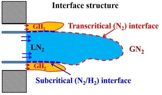
  • The LES study of classical cryogenic injection of liquid nitrogen injected coaxially with warm hydrogen jet, case 8, showed some interesting thermodynamic phenomena, such as the condensation of H 2 as well as cooling effects in the two-phase layer around the liquid core, which demonstrates the subcritical nature of the interface.
  • Another interesting observed phenomenon for case 8 is related to the mixing of N 2 and H 2 , which led to locally increased mixture critical points. Therefore, due to the mixing process around the liquid core interface, some flow zones may move from the supercritical mixing regime to the subcritical phase change regime inducing condensation and evaporation.
  • The numerical results were finally compared with available experimental data [43] and published numerical studies [40], with satisfactory agreement. Moreover, we confirmed the importance of using a powerful real fluid EoS. The current investigations illustrated that the SRK EoS had a better prediction of the fluid density compared to the PR EoS, corroborating the results reported by [40].
  • Finally, compared to our previous studies [8,9,66], the computational efficiency, accuracy, and robustness of this proposed tabulated RFM model as a remedy to the direct evaluation of costly phase equilibrium solver were confirmed.

Author Contributions

Conceptualization, methodology and formal analysis, S.J., H.G., C.H. and J.-C.d.H.; validation and investigation, S.J; writing—original draft preparation, S.J; writing—review, S.J., H.G., C.H. and J.-C.d.H.; supervision, C.H. and J.-C.d.H.; All authors have read and agreed to the published version of the manuscript.

Funding

This research received no external funding.

Institutional Review Board Statement

Not applicable.

Informed Consent Statement

Not applicable.

Data Availability Statement

Data available on request due to restrictions.

Acknowledgments

The authors would like to acknowledge Angela Di Lella for her support and for providing the thermodynamic solver, IFPEN-CARNOT.

Conflicts of Interest

The author(s) declare no potential conflicts of interest with respect to the research, authorship, and/or publication of this article.

Appendix A

ρ = p α p ρ p
e = p α p ρ p e p ρ
λ = p α p ρ p λ p ρ
C p = p α p ρ p C p p ρ
C v = p α p ρ p C v p ρ
μ p = p α p ρ p μ p ρ
1 ρ C s , m i x , w o o d 2 = p α p ρ p C s , m i x 2
Figure A1. Flow chart of the thermodynamic solver for generating the properties table.
Energies 14 05621 g0a1
Figure A2. Flow chart of the RFM PISO algorithm. (See Section 2).
Energies 14 05621 g0a2
Figure A3. Comparison and verification of the thermodynamic model used in this study with the data of NIST [38] for different EoSs for density, heat capacity, sound speed, and viscosity, respectively, for pure H 2 . PR, and SRK refer to the Peng Robinson, and Soave–Redlich–Kwong equations of state.
Energies 14 05621 g0a3

References

  1. Sirignano, W.A.; Delplanque, J.P. Transcritical vaporization of liquid fuels and propellants. J. Propul. Power 1999, 15, 806–902. [Google Scholar]
  2. Chehroudi, B.; Talley, D.; Mayer, W.; Branam, R.; Smith, J.J.; Schik, A.; Oschwald, M. Understanding Injection into High Pressure Supercritical Environments. In Proceedings of the Fifth International Symposium on Liquid Space Propulsion, Long Life Combustion Devices Technology, Huntsville, AL, USA, 27–30 October 2003; NASA Marshall Spaceflight Center: Huntsville, AL, USA, 2003. [Google Scholar]
  3. Mayer, W.O.; Schik, A.; Schaffler, M.; Tamura, H. Injection and mixing processes in high-pressure liquid oxygen/gaseous hydrogen rocket combustors. J. Propul. Power 2000, 16, 823–828. [Google Scholar] [CrossRef]
  4. Crua, C.; Manin, J.; Pickett, L.M. On the transcritical mixing of fuels at diesel engine conditions. Fuel 2017, 208, 535–548. [Google Scholar] [CrossRef] [Green Version]
  5. Jofre, L.; Urzay, J. Transcritical diffuse-interface hydrodynamics of propellants in high-pressure combustors of chemical propulsion systems. Prog. Energy Combust. Sci. 2021, 82, 100877. [Google Scholar] [CrossRef]
  6. Banuti, D.T. Crossing theWidom-line—Supercritical pseudo-boiling. J. Supercrit. Fluids 2015, 98, 12–16. [Google Scholar] [CrossRef]
  7. Bellan, J. Supercritical (and subcritical) fluid behavior and modeling: Drops, streams, shear and mixing layers, jets and sprays. Prog. Energy Combust. Sci. 2000, 26, 329–366. [Google Scholar] [CrossRef] [Green Version]
  8. Yi, P.; Yang, S.; Habchi, C.; Lugo, R. A multicomponent real-fluid fully com- pressible four-equation model for two-phase flow with phase change. Phys. Fluids 2019, 31, 026102. [Google Scholar] [CrossRef]
  9. Yang, S.; Yi, P.; Habchi, C. Real-fluid injection modeling and LES simulation of the ECN Spray A injector using a fully compressible two-phase flow approach. Int. J. Multiph. Flow 2020, 122, 103145. [Google Scholar] [CrossRef]
  10. Dahms, R.N.; Oefelein, J.C. On the transition between two-phase and single-phase interface dynamics in multicomponent fluids at supercritical pressures. Phys. Fluids 2013, 25, 092103. [Google Scholar] [CrossRef]
  11. Ma, P.C.; Lv, Y.; Ihme, M. An entropy-stable hybrid scheme for simulations of transcritical real-fluid flows. J. Comput. Phys. 2017, 340, 330–357. [Google Scholar] [CrossRef]
  12. Ma, P.C.; Wu, H.; Banuti, D.T.; Ihme, M. On the numerical behavior of diffuse-interface methods for transcritical real-fluids simulations. Int. J. Multiph. Flow 2019, 113, 231–249. [Google Scholar] [CrossRef]
  13. Andrews, T. The Bakerian Lecture—On the Continuity of the Gaseous and Liquid States of Matter. Philos. Trans. R. Soc. Lond. 1869, 159, 575. [Google Scholar]
  14. Lapenna, P.E. Thermodynamic Small Scales in Transcritical Turbulent Jets. AIAA J. 2021. [Google Scholar] [CrossRef]
  15. Doehring, A.; Kaller, T.; Schmidt, S.J.; Adams, N.A. Large-eddy simulation of turbulent channel flow at transcritical states. Int. J. Heat Fluid Flow 2021, 89, 108781. [Google Scholar] [CrossRef]
  16. Ningegowda, B.M.; Rahantamialisoa, F.N.Z.; Pandal, A.; Jasak, H.; Im, H.G.; Battistoni, M. Numerical Modeling of Transcritical and Supercritical Fuel Injections Using a Multi-Component Two-Phase Flow Model. Energies 2020, 13, 5676. [Google Scholar] [CrossRef]
  17. Gallo, P.; Corradini, D.; Rovere, M. Widom line and dynamical crossovers as routes to understand supercritical water. Nat. Commun. 2014, 5, 5806. [Google Scholar] [CrossRef] [Green Version]
  18. Xu, L.; Kumar, P.; Buldyrev, S.V.; Chen, S.-H.; Poole, P.H.; Sciortino, F.; Stanley, H.E. Relation between the Widom line and the dynamic crossover in systems with a liquid–liquid phase transition. Proc. Natl. Acad. Sci. USA 2005, 102, 16558–16562. [Google Scholar] [CrossRef] [PubMed] [Green Version]
  19. Michelsen, M.L. The isothermal flash problem, Part I. Phase split calculation. Fluid Phase Equilib. 1982, 9, 1–19. [Google Scholar] [CrossRef]
  20. Ayyappan, D.; Vaidyanathan, A.; Muthukumaran, C.K.; Nandakumar, K. Transition of subcritical liquid jets in single and multicomponent systems. Phys. Fluids 2018, 30, 104106. [Google Scholar] [CrossRef]
  21. Mirjalili, S.; Jain, S.S.; Dodd, M. Interface-Capturing Methods for Two-Phase Flows: An Overview and Recent Developments; Center for Turbulence Research Annual Research Briefs, Stanford University: Stanford, CA, USA, 2017; pp. 117–135. [Google Scholar]
  22. Saurel, R.; Pantano, C. Diffuse-Interface Capturing Methods for Compressible Two-Phase Flows. Annu. Rev. Fluid Mech. 2018, 50, 105–130. [Google Scholar] [CrossRef] [Green Version]
  23. Cahn, J.; Hilliard, J. Free energy of a nonuniform system. I. Interfacial free energy. J. Chem. Phys. 1958, 28, 258–267. [Google Scholar] [CrossRef]
  24. Baer, M.; Nunziato, J. A two-phase mixture theory for the deflagration-to-detonation transition (DDT) in reactive granular materials. Int. J. Multiph. Flow 1986, 12, 861–889. [Google Scholar] [CrossRef]
  25. Pantano, C.; Saurel, R.; Schmitt, T. An oscillation free shock-capturing method for compressible van der Waals supercritical fluid flows. J. Comput. Phys. 2017, 335, 780–811. [Google Scholar] [CrossRef] [Green Version]
  26. Hirt, C.W.; Nichols, B.D. Volume of uid (vof) method for the dynamics of free boundaries. J. Comput. Phys. 1981, 39, 201–225. [Google Scholar] [CrossRef]
  27. Scardovelli, R.; Zaleski, S. Analytical relations connecting linear interfaces and volume fractions in rectangular grids. J. Comput. Phys. 2000, 164, 228–237. [Google Scholar] [CrossRef]
  28. Mastrone, M.N.; Hartono, E.A.; Chernoray, V.; Concli, F. Oil distribution and churning losses of gearboxes: Experimental and numerical analysis. Tribol. Int. 2020, 151, 106496. [Google Scholar] [CrossRef]
  29. Peng, Q.; Gui, L.; Fan, Z. Numerical and experimental investigation of splashing oil flow in a hypoid gearbox. Eng. Appl. Comput. Fluid Mech. 2018, 12, 324–333. [Google Scholar] [CrossRef] [Green Version]
  30. Chiapolino, A.; Boivin, P.; Saurel, R. A simple phase transition relaxation solver for liquid-vapor flows. Int. J. Numer. Methods Fluids 2017, 83, 583–605. [Google Scholar] [CrossRef] [Green Version]
  31. Zein, A.; Hantke, M.; Warnecke, G. Modeling phase transition for compressible two-phase flows applied to metastable liquids. J. Comput. Phys. 2010, 229, 2964–2998. [Google Scholar] [CrossRef]
  32. Mirjalili, S.; Ivey, C.B.; Mani, A. Comparison between the diffuse interface and volume of fluid methods for simulating two-phase flows. Int. J. Multiph. Flow 2019, 116, 221–238. [Google Scholar] [CrossRef] [Green Version]
  33. Osher, S.; Fedkiw, R.P. Level set methods: An overview and some recent results. J. Comput. Phys. 2001, 169, 463–502. [Google Scholar] [CrossRef] [Green Version]
  34. Sethian, J.A.; Smereka, P. Level set methods for fuid interfaces. Annu. Rev. Fluid Mech. 2003, 35, 341–372. [Google Scholar] [CrossRef] [Green Version]
  35. Umemura, A.; Shinjo, J. Detailed SGS atomization model and its implementation to two-phase flow LES. Combust. Flame 2018, 195, 232–252. [Google Scholar] [CrossRef]
  36. Legier, J.P.; Poinsot, T.; Veynante, D. Dynamically thickened flame LES model for premixed and non-premixed turbulent combustion. In Proceedings of the Summer Program, Stanford, CA, USA, 2–27 July 2000; Center for Turbulence Research, NASA Ames/Stanford University: Stanford, CA, USA, 2000; pp. 157–168. [Google Scholar]
  37. Devassy, B.M.; Habchi, C.; Daniel, E. Atomization Modelling of Liquid Jets Using a Two-Surface-Density Approach. At. Sprays 2015, 25, 47–80. [Google Scholar] [CrossRef]
  38. Linstrom, P; Mallard, W. The NIST Chemistry WebBook: A Chemical Data Resource on the Internet. J. Chem. Eng. Data 2001, 46, 1059–1063. [Google Scholar] [CrossRef]
  39. Banuti, D.; Hannemann, K. Efficient multiphase rocket propellant injection model with high quality equation of state. In Proceedings of the 4th Space Propulsion Conference, Cologne, Germany, 19–22 May 2014. [Google Scholar]
  40. Matheis, J.; Müller, H.; Hickel, S.; Pfitzner, M. Large-Eddy Simulation of Cryogenic Jet Injection at Supercritical Pressures. High-Press. Flows Propuls. Appl. 2020, 260, 531–570. [Google Scholar]
  41. Multi-component vapor-liquid equilibrium model for LES and application to ECN spray A. arXiv 2016, arXiv:1609.08533.
  42. Lacaze, G.; Schmitt, T.; Ruiz, A.; Oefelein, J.C. Comparison of energy, pressure-and enthalpy-based approaches for modeling supercritical flows. Comput. Fluids 2019, 181, 35–56. [Google Scholar] [CrossRef] [Green Version]
  43. Oschwald, M.; Schik, A.; Klar, M.; Mayer, W. Investigation of coaxial LN2/GH2-injection at supercritical pressure by spontaneous Raman scattering. In Proceedings of the 35th Joint Propulsion Conference and Exhibit, Los Angeles, CA, USA, 20–24 June 1999. [Google Scholar]
  44. Michelsen, M.L. The isothermal flash problem, Part II. Phase split calculation. Fluid Phase Equilib. 1982, 9, 21–40. [Google Scholar] [CrossRef]
  45. Koukouvinis, P.; Vidal-Roncero, A.; Rodriguez, C.; Gavaises, M.; Pickett, L. High pressure/high temperature multiphase simulations of dodecane injection to nitrogen: Application on ECN Spray—A. Fuel 2020, 275, 117871. [Google Scholar] [CrossRef]
  46. Yi, P.; Jafari, S.; Yang, S.; Habchi, C. Numerical analysis of subcritical evaporation and transcritical mixing of droplet using a tabulated multicomponent vapor-liquid equilibrium model. In Proceedings of the ILASS—Europe 2019, 29th Conference on Liquid Atomization and Spray Systems, Paris, France, 2–4 September 2019. [Google Scholar]
  47. Brown, S.; Peristeras, L.; Martynov, S.; Porter, R.T.J.; Mahgerefteh, H.; Nikolaidis, I.; Boulougouris, G.; Tsangaris, D.; Economou, I. Thermodynamic interpolation for the simulation of two-phase flow of non-ideal mixtures. Comput. Chem. Eng. 2016, 95, 49–57. [Google Scholar] [CrossRef]
  48. Azimian, A.R.; Arriagada, J.; Assadi, M. Generation of steam tables using artificial neural networks. Heat Transf. Eng. 2004, 25, 41–51. [Google Scholar] [CrossRef]
  49. Lorenzo, M.; De Lafon, P.; Di Matteo, M.; Pelanti, M.; Seynhaeve, J.M.; Bartosiewicz, Y. Homogeneous two-phase flow models and accurate steam-water table look-up method for fast transient simulations. Int. J. Multiph. Flow 2017, 95, 199–219. [Google Scholar] [CrossRef]
  50. Fang, Y.; De Lorenzo, M.; Lafon, P.; Poncet, S.; Bartosiewicz, Y. An Accurate and Efficient Look-up Table Equation of State for Two-phase Compressible Flow Simulations of Carbon Dioxide. Ind. Eng. Chem. Res. 2018, 57, 7676–7691. [Google Scholar] [CrossRef]
  51. Foll, F.; Hitz, T.; Muller, C.; Munz, C.-D.; Dumbser, M. On the use of tabulated equations of state for multi-phase simulations in the homogeneous equilibrium limit. Shock Waves 2019, 29, 769–793. [Google Scholar] [CrossRef]
  52. Praneeth, S.; Hickey, J.-P. Uncertainty quantification of tabulated supercritical thermodynamics for compressible Navier–Stokes solvers. arXiv 2018, arXiv:1801.06562. [Google Scholar]
  53. Saha, S.; Carroll, J.J. The isoenergetic-isochoric flash. Fluid Phase Equilib. 1997, 138, 23–41. [Google Scholar] [CrossRef]
  54. Richards, K.J.; Senecal, P.K.; Pomraning, E. Converge 3.0; Convergent Science: Madison, WI, USA, 2021; Available online: https://convergecfd.com/ (accessed on 15 January 2019).
  55. Chung, T.H.; Ajlan, M.; Lee, L.L.; Starling, K.E. Generalized multi-parameter correlation for non-polar and polar fluid transport properties. Ind. Eng. Chem. Res. 1988, 27, 671–679. [Google Scholar] [CrossRef]
  56. Sagaut, P. Large-Eddy Simulation for Incompressible Flows, 3rd ed.; Scientific Computation; Springer: Berlin/Heidelberg, Germany; New York, NY, USA, 2005. [Google Scholar]
  57. Peng, D.-Y.; Robinson, D.B. A new two-constant equation of state. Ind. Eng. Chem. Fundam. 1976, 15, 59–64. [Google Scholar] [CrossRef]
  58. Soave, G. Equilibrium constants from a modified redlichkwong equation of state. Chem. Eng. Sci. 1972, 27, 1197–1203. [Google Scholar] [CrossRef]
  59. Ware, C.; Knight, W.; Wells, D. Memory intensive statistical algorithms for multibeam bathymetric data. Comput. Geosci. 1991, 17, 985–993. [Google Scholar] [CrossRef]
  60. Streett, W.B.; Calado, J.C.G. Liquid-vapour equilibrium for hydrogen + nitrogen at temperatures from 63 to 110 k and pressures to 57 mpa. J. Chem. Thermodyn. 1978, 10, 1089–1100. [Google Scholar] [CrossRef]
  61. Boyd, B.; Jarrahbashi, D. A diffuse-interface method for reducing spurious pressure oscillations in multicomponent transcritical flow simulations. Comput. Fluids 2021. [Google Scholar] [CrossRef]
  62. Issa, R.I.; Gosman, A.D.; Watkins, A.P. The Computation of Compressible and Incompressible Recirculating Flows by a Non-Iterative Implicit Scheme. J. Comput. Phys. 1986, 62, 66–82. [Google Scholar] [CrossRef]
  63. Patankar, S.V. Numerical Heat Transfer and Fluid Flow; Hemisphere Publishing Corporation: Washington, DC, USA, 1980. [Google Scholar]
  64. Poormahmood, A.; Farshchi, M. Numerical study of the mixing dynamics of trans- and supercritical coaxial jets. Phys. Fluids 2020, 32, 125105. [Google Scholar] [CrossRef]
  65. Yang, S. Modeling of Diesel Injection in Subcritical and Supercritical Conditions. Ph.D. Thesis, University of Paris-Saclay, Gif-sur-Yvette, France, 2019. [Google Scholar]
  66. Yang, S.; Habchi, C. Real-fluid phase transition in cavitation modeling considering dissolved non-condensable gas. Phys. Fluids 2020, 32, 032102. [Google Scholar]
Figure 1. Experimental images (adapted from [2]) of pure liquid N 2 injection from subcritical to supercritical pressure conditions (ac). A schematic showing the three (subcritical (a), transcritical (b), and supercritical (c)) isobaric paths for a single component (ac). Figure (d) denotes different modeling regimes with regard to the variation of Tr and Pr, schematically. The variations of the density, and isobaric heat capacity of pure nitrogen at transcritical condition calculated in this study, using PR EoS, are shown in Figure (e) where liquid-like properties are colored in blue and gas-like properties are colored in red.
Energies 14 05621 g001
Figure 6. The vapor–liquid equilibrium of H 2 - N 2 calculated in this study using SRK-EoS compared to the experimental data [60].
Energies 14 05621 g006
Figure 7. Different properties variations as a function of temperature and H 2 mass fraction for binary mixture of H 2 - N 2 at P = 4 MPa.
Energies 14 05621 g007
Figure 8. (a) Flow chart of the decoupled flow solver and thermodynamic solver used in [9] for the SIMPLE algorithm and (b) the proposed flow chart of the fully coupled flow solver and thermodynamic solver applied in the SIMPLE algorithm.
Energies 14 05621 g008
Figure 9. Case 1, comparison of different results for the density, temperature, pressure, velocity, heat capacity, and gas volume fraction, respectively, using PR-EoS, for the transcritical shock tube between the presented model in this study named the RFM and Ma et al. [11] at 500 μ s. CFL = 0.1 for the RFM model and CFL = 0.8 for the Ma model. The thin dashed lines are the initial conditions.
Energies 14 05621 g009
Figure 10. The impacts of pressure variations on the property evolution for the transcritical shock tube test case, defined as case 1:3 in Table 2, using PR-EoS, on the (a) pressure profile, (b) temperature profile, (c) density profile, and (d) isobaric heat capacity, using the SIMPLE numerical scheme, at t = 500 μ s. A comparison between the SIMPLE and PISO schemes for cases (3–4) shows good agreement between them at this condition.
Energies 14 05621 g010aEnergies 14 05621 g010b
Figure 11. Setup of transcritical jet simulation.
Energies 14 05621 g011
Figure 12. Case 5 instantaneous contour plots of density, heat capacity, and phase indicator (PHI); PHI = 0 designates a liquid state, and PHI = 1 designates a gas state.
Energies 14 05621 g012
Figure 13. Case 5 instantaneous contour plots of temperature and vorticity fields at transcritical condition at t = 5 ms. The position of interface between the liquid-like and gas-like at the pseudo boiling line at the temperature contour, is determined by C p , m a x iso-line, colorized in white. The C p , m a x at the interface acts like a thermal shield for the jet.
Energies 14 05621 g013
Figure 14. Case 6, instantaneous contour plots of temperature and isobaric heat for supercritical nitrogen injection at T = 150 K and P = 6 MPa after t = 5 ms.
Energies 14 05621 g014
Figure 15. Case 7, instantaneous contour plots of the density, temperature, and isobaric heat capacity for supercritical nitrogen injection at T = 135 K and P = 4 MPa after t = 5 ms. Isobaric heat capacity (Cp) reduces continuously from liquid jet to the chamber, and there is no peak at Cp, no thermal shield at the interface, no thermal shield, and it has a symmetrical distribution. Hence, there is no crossing of the Widom line, which proves that the jet is in the supercritical regime.
Energies 14 05621 g015
Figure 16. Case 8: (Left) Schematic of the injector experimental configuration: blue and red colors indicate L N 2 and G H 2 canals, respectively. (Right) Computational domain in the central cut-section of the simulated 3D geometry. AMR is used based on the criterion of the minimum velocity of 0.1 m/s.
Energies 14 05621 g016
Figure 17. Distribution of mixture density (a), and H 2 mass fraction (b).
Energies 14 05621 g017
Figure 18. Distribution of H 2 density, temperature, and phase indicator (in the central cut-section) using the two different EoS at t = 4.5 ms. PHI = 0, 1, and 2 denote liquid, gas, and two-phase states.
Energies 14 05621 g018
Figure 19. Temperature H 2 -composition phase diagram for a binary mixture of N 2 - H 2 at P = 4 MPa, calculated by PR-EoS, compared with [40], used PR-EoS, along with the adiabatic mixing temperature (AMT).
Energies 14 05621 g019
Figure 20. Distribution of the mixture heat capacity (Left) and reduced temperature. T r = T / T c , m i x (Right) where T c , m i x is the mixture critical temperature. The subcritical region for the mixture where T r < 1 is colorized by white.
Energies 14 05621 g020
Figure 21. Radial reduced temperature and gas volume fraction profiles at X = 3 mm after t = 3 ms. The radial axis is displayed in Figure 20b.
Energies 14 05621 g021
Figure 22. Different properties contours plotted at t = 4 ms as (a) mixture gas volume fraction, (b) mixture compressibility factor, and (c) mixture sound speed.
Energies 14 05621 g022aEnergies 14 05621 g022b
Figure 23. Axial and radial density profiles compared to the experimental [43] and the LES study by Matheis et al. [40]. D i = 1.9 mm.
Energies 14 05621 g023aEnergies 14 05621 g023b
Figure 24. Pressure oscillations of the flow field in the chamber at the central cut section. The initial ambient pressure in the chamber is P = 4 MPa.
Energies 14 05621 g024
Table 1. Parameters for cubic equations of state (index c stands for critical value).
EOS δ 1 δ 2 ( a c ) i m i b i
PR 1 + 2 1+ 2 0.45727 R 2 T c 2 P c 0.37464 + 1.54226 ω 0.26992 ω 2 0.0778 R T c P c
SRK10 0.42747 R 2 T c 2 P c 0.48508 + 1.5517 ω 0.15613 ω 2 0.08664 R T c P c
Table 2. Initial conditions for pure N 2 transcritical shock tube test cases for different pressures.
P L (MPa) P R (MPa) T L (K) T R (K) U L = U R (m/s)Numerical Scheme
Case 16061582240 S I M P L E
Case 24061582240 S I M P L E
Case 32061582240 S I M P L E
Case 42061582240 P I S O
Table 3. Operating conditions for the transcritical cryogenic N 2 injection similar to Mayer’s experimental study [3].
T inj (K) T ch (K) P ch (MPa)
Case 5126.92986
Case 61502986
Case 71352984
Publisher’s Note: MDPI stays neutral with regard to jurisdictional claims in published maps and institutional affiliations.

