1. Introduction
Nanofluid is a mixture obtained by mixing nanoparticles with ordinary heat energy transfer fluids such as oil, glycol, water, ethylene glycol, etc. Nanoparticles can be prepared on a small scale (laboratories) as well as on a large scale (in industries). The usual size of nanoparticles lies in the range 1–100 nm [
1]. Nanoparticles can be made from metals such as Al, Cu, Au, and Ag, metal oxides such as Fe
3O
4, CuO, TiO
2, and Al
2O
3, nitrides such as SiN and AlN, and carbides such as SiC, etc. These nanometer-sized particles can be added in a minute amount to augment the heat energy transfer rate due to their tremendous thermal conductivities [
2,
3]. Due to nanometer-sized geometry, the nanoparticles can easily mix with the base fluid [
4]. A literature study suggests that there are two main techniques to model nanofluids. In the first type, the nanoparticles are distributed uniformly throughout the host fluid. The nanofluids’ thermophysical characteristics lead to the boundary-layer equations, which can be used to study the nanoparticles’ effects. On the other hand, the models created to consider the nanoparticles’ interaction with the base fluid are known as two-phase models, and are known as the second case of the nanofluid model [
5]. Tewari and Das [
6] studied the single-phase model, while Buongiorno [
7] has investigated the two-phase nanoparticle model. A study was also performed by Vajravelu and Mukhopadhayay [
8] on a single-phase model.
The use of nanoparticles varies from a small scale in laboratories to a very large scale in industries. Due to high thermal conductivities, nanofluids are used for cooling purposes in transformers, cooling chambers, and in nuclear reactors. For medical purposes, they are used to design different surgery equipment to kill tumor cells. In electronic machines, the heat generated during their operation can also be reduced by using different nanofluids. Tewari and Das’s [
6] model has been further investigated by many researchers to elaborate on the thermal features of different nanofluids [
9,
10,
11,
12].
The investigation of heat energy transfer during non-Newtonian fluid flow on stretched surfaces has recently gained significant attention [
13]. Due to different kinds of flow in real situations, a single constitutive relation which relates the shear stress and shear rate is insufficient to investigate the non-Newtonian fluid properties [
14]. There are some viscoelastic fluids which show polar effects, called couple stress fluids, which simplify the traditional theories for investigation [
15]. For this kind of fluid, the constitutive relations associate the skew-symmetric portion of the stress tensor with the angular velocity, and the couple stress with the gradient in angular velocity [
16]. Eringen [
17] called the polar fluids micropolar fluids. The theory of dipolar fluids was developed by Bleustein and Green [
18]. If the polar fluid is in such a state that the cosserat triad is rigidly attached to the medium, then it is known as a couple stress fluid. The polar and dipolar fluids are considered in the couple stress theory which Stokes created [
19]. The Navier–Stokes equations cannot describe such fluids due to their stress tensor non-symmetric nature. Examples include lubricants that contain polymer preservative to some extent, synthetic fluids, blood, and electro-rheological fluids [
20].
Due to the relevance of couple stress fluids in the chemical trade and various machineries, a good number of researchers have given attention to the study of their flow and associated properties. Hayat et al. [
21] worked out the melting process in investigating the heat energy transfer for this kind of fluid at the stagnation point. Ramzan et al. [
22] examined the accumulative effects of heating and magnetic field on the couple stress fluid three-dimensional flow. Srinivasacharya and Kaladhar [
23] have studied both Duofour and Soret effects on the convective flow in a porous medium. Turkyilmazoglu [
24] analytically investigated two-dimensional flow on an extended surface. Furthermore, Hayat et al. [
25] employed the two-phase nanofluid model to investigate the combined impacts of convective boundary conditions and magnetic field on the couple stress fluid three-dimensional flow on a non-linear enlarged surface. Pordanjani et al. [
26] examined the impact of radiation and magnetic field on entropy generation and convective thermal energy nanofluid flow rate through a rectangular container and investigated the influence of pertinent parameters on the flow features. Additionally, Ramzan [
27] has investigated the effects of Joule heating, viscous dissipation, and applied magnetic field on the 3D couple stress nanofluid flow. The heat transfer augmentation characteristics of alumina water nanofluid in the presence of a homogeneous magnetic field flowing through a rectangular channel was investigated by Bagherzadeh et al. [
28].
There are different mechanisms by which energy can transfer from one place to another. In different manufacturing techniques, the heat transfer through radiation is more efficient and practical than convective heat transfer when there is a large temperature difference between the ambient fluid and the surface [
29]. To simplify the situation, the majority of researchers have applied the Rosseland approximation to study the effects of linear radiation [
30]. Jamshed et al. [
31] studied the impacts of solar radiation transport and slip condition on the convective thermal features of an unsteady flow of Casson nanofluid. Sheikholeslami [
32] investigated the effects of linear thermal radiations on nanofluid flow through an elliptic cylinder. Sajid et al. [
33] examined the effects of multiple convective sufrace boundary conditions, non-linear thermal radiations, exponential heat source, and viscous dissipation on incompressible micropolar fluid motion through a porous stretching surface. Dogonchi et al. [
34] used a porous channel to study the impacts of thermal radiations on the heat transfer during nanofluid migration. In the majority of these investigations, the researchers applied linear thermal radiation terms to make the situation simple. To obtain the complete knowledge of the heat transfer during nanofluid flow, it is very important to take into account the impacts produced due to the inclusion of non-linear thermal radiations [
35,
36,
37,
38,
39].
The wide range of applications of nanofluids depend upon the geometry of the problem under consideration. Heat transfer analysis of the motion of different nanofluids has been performed by many researchers using different geometries. Devakar et al. [
40] studied non-Newtonian fluid motion through a square duct past a permeable medium. Srinivasacharya and Shafeeurrahman [
41] investigated the nanofluid flow between concentric cylinders. Rashidi et al. [
42] investigated the fluid flow on a rotatory sheet, and derived a semi-analytic solution. Khan and Pop [
43] studied the nanofluid flow over a stretching sheet. The flow over a stretching sheet has attracted significant attention in the last few years due to its unique nature and industrial applications. Different studies on stretching sheets can be found in detail in the papers [
44,
45,
46,
47,
48,
49]. Gosh et al. [
50] used the Tiwari and Das model to investigate the couple stress magnetite–water-based nanofluid motion near a bi-directional stretchable surface incorporating the effects due to non-linear thermal radiations. Lund et al. [
51] discussed the dual and symmetrical solution of hybrid nanofluid flow past a stretching surface. They analyzed the rotating frame’s impact on the hybrid nanofluid flow. A more recent survey of the hybrid nanofluid flow is discussed by Ali et al. [
52,
53].
The present article deals with the three-dimensional nanofluid (water-based) flow of the boundary layer over a rotating surface considering the impacts of both thermal radiations and couple stress. The study of three-dimensional problem gives more insight into the actual scenario as compared to two-dimensional investigations. The Tewari and Das [
6] model is used. The modeled equations are converted to a simple set of non-linear ODEs through suitable similarity transformations. From the obtained solution, we have found that the numerical results are in agreement with the analytical results obtained through HAMS. The results of the study are explained with the help of different graphs as well as tables.
2. Mathematical Model of the Problem
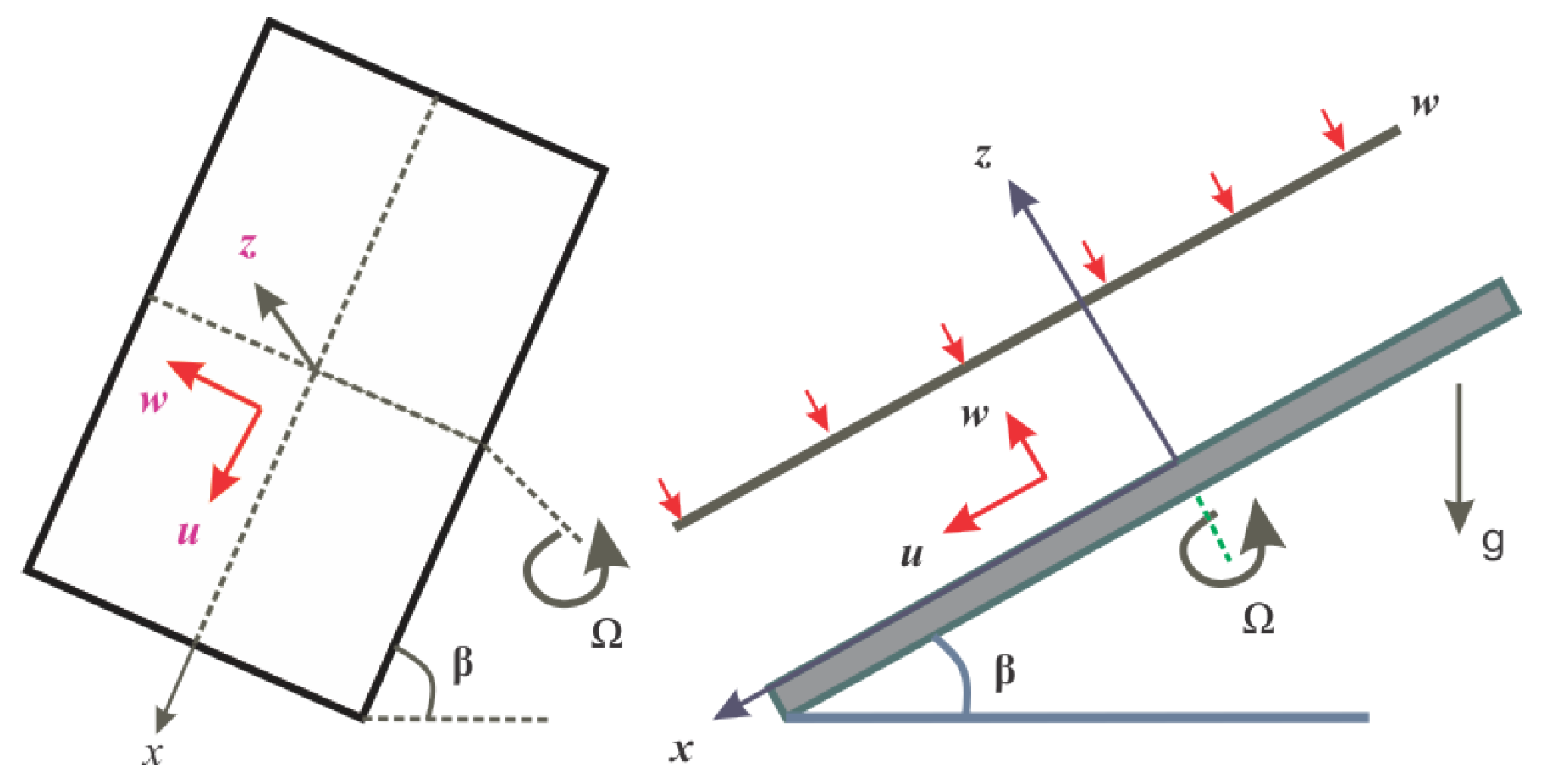
The impacts of thermal radiations on the three-dimensional and steady boundary-layer laminar flow of couple stress water-based nanofluid (incompressible) over a rotating surface are considered in the current study. The geometry of the problem is sketched in
Figure 1. The nanoparticles are supposed to be in equilibrium with the base fluid. Furthermore, no slip at the boundary occurs.
The model equations for the nanofluid flow are [
54]:
Here,
,
, and
p are, respectively, the density, velocity, and pressure of the assumed fluid. The symbols
and
represent the body force and body couple per unit mass, respectively. The symbols
and
are the coefficients of viscosity. The stress tensor
and the deformation rate tensor
[
54] are related by the following constitutive relation:
The constitutive relation for the couple stress tensor is
Here,
is the spinning vector,
denotes the spin tensor,
m is the trace of the couple stress tensor, (
) is the body couple, and
is the viscosity coefficient of the couple stress. The material constants
,
,
n, and
satisfy the inequalities
,
,
, and
, respectively.
The single-phase nanofluid approach and the effective fluid properties of nanofluid in spherical symmetry are considered. These nanofluid properties are defined as [
11]:
These model relations for the incompressible fluid flow, in the absence of body force and couple stress effects [
54] reduce to the following relations:
By using
and then employing the Tiwari and Das model [
6], the model equations in the final form are [
54]:
Here,
are the nanofluid kinematic and couple stress viscosities,
(
) is the nanofluid viscosity (density),
is the nanofluid thermal conductivity (specific heat capacity).
The boundary conditions for Equations (
8)–(
12) are
5. Results and Discussion
This section is devoted to discussing the achieved results. The results obtained from the solution of the system of coupled ODEs are explained by displaying different graphs. In these plots, the variations in the velocity components, fluid temperature, and Nusselt number with respect to increasing values of the pertinent parameters are displayed.
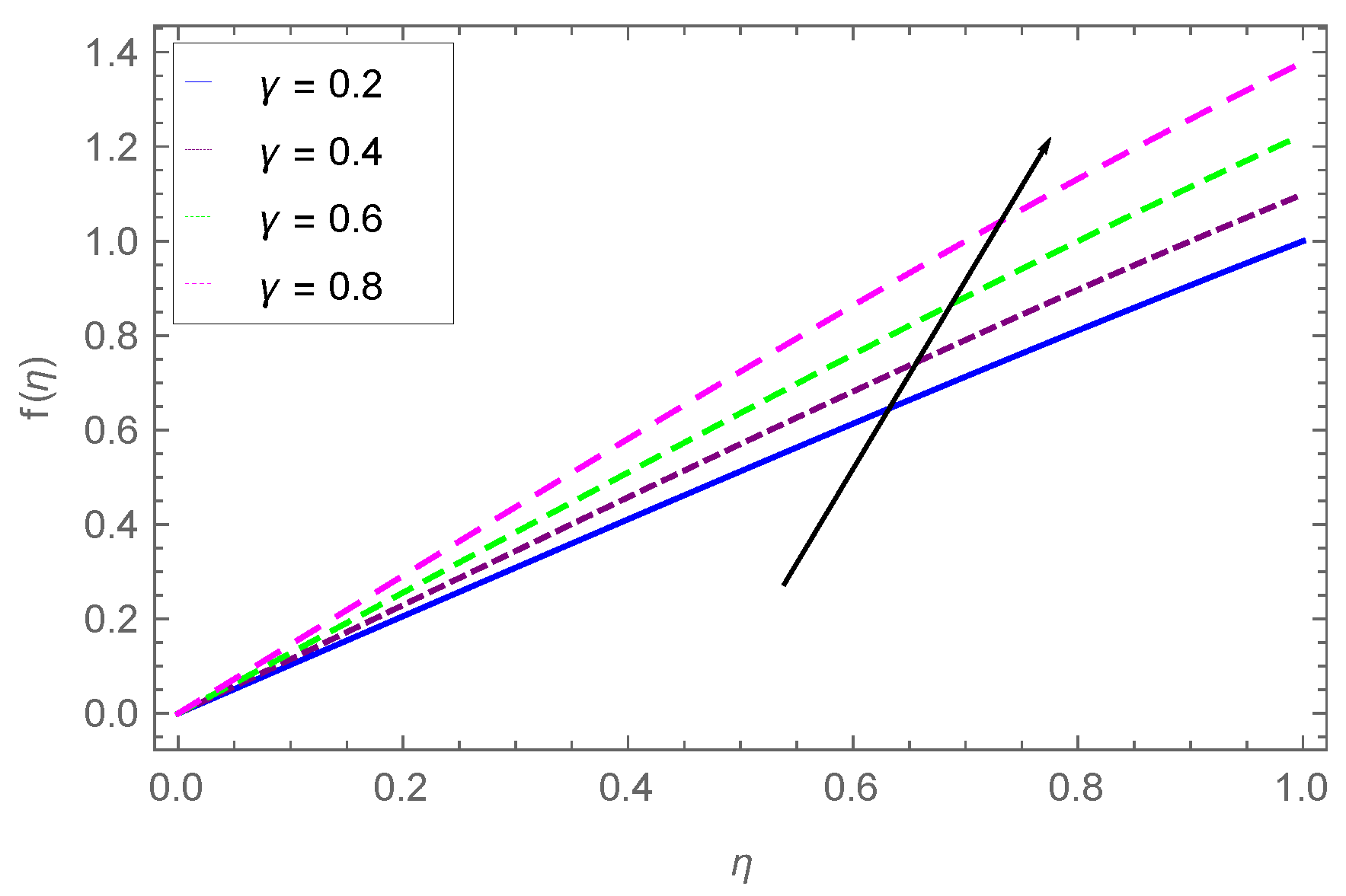
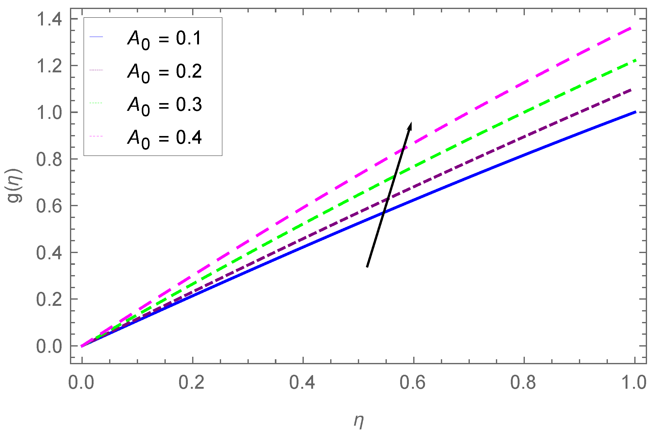
The effect of
(thickness parameter) on the velocity profile is displayed in
Figure 3. The increasing values of the thickness parameter augment the fluid velocity. These variations are more effective beyond
, and are maximum at
. Physically, when
increases, the kinematic viscosity decreases and the rotation rate increases, which increases the flow along the x-direction, and as a result the velocity profile increases.
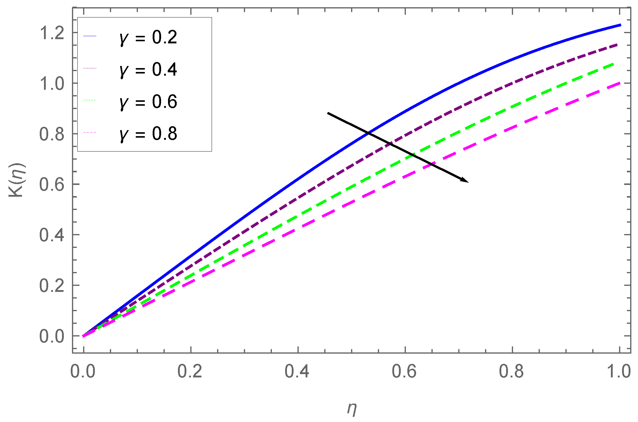
The impact of
on the draining velocity in the x-direction is displayed in
Figure 4. The rising values of the thickness parameter decrease the velocity profile due to the higher values of the rotation rate. The higher values of
intensify the flow in the x-direction, but the draining flow reverses, and as a result the velocity profile declines. These variations are much more effective beyond
, and change with higher values of
.
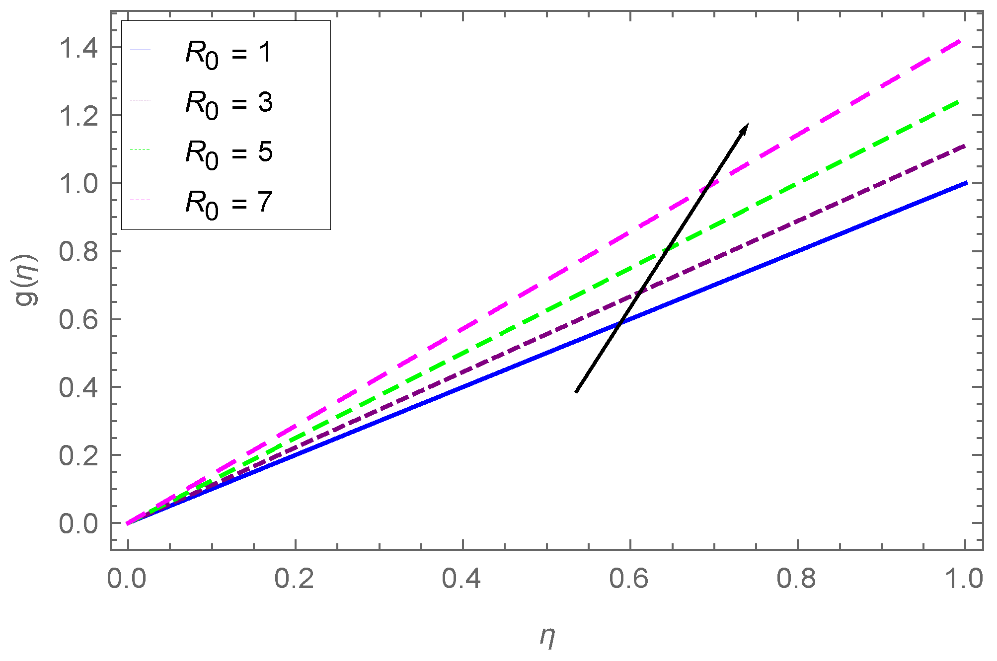
The influence of
on the induced flow in the y-direction is displayed in
Figure 5. The figure shows that the larger values of the thickness parameter increase the velocity profile, and these variations are more effective beyond
. The spacing between different curves increases with changing
. Physically, the increasing values of the thickness parameter increase due to larger values of
, which further increases the rotation in the flow, and results an increase in the induced flow in the y-direction.
Figure 6 plots the fluid temperature
for varying
. At fixed
, there is approximately a direct relation between
and
up to about
. The figure also shows that there is an increasing trend in
with the higher values of
. This increasing trend is more prominent for the highest value of
in the range from
up to
.
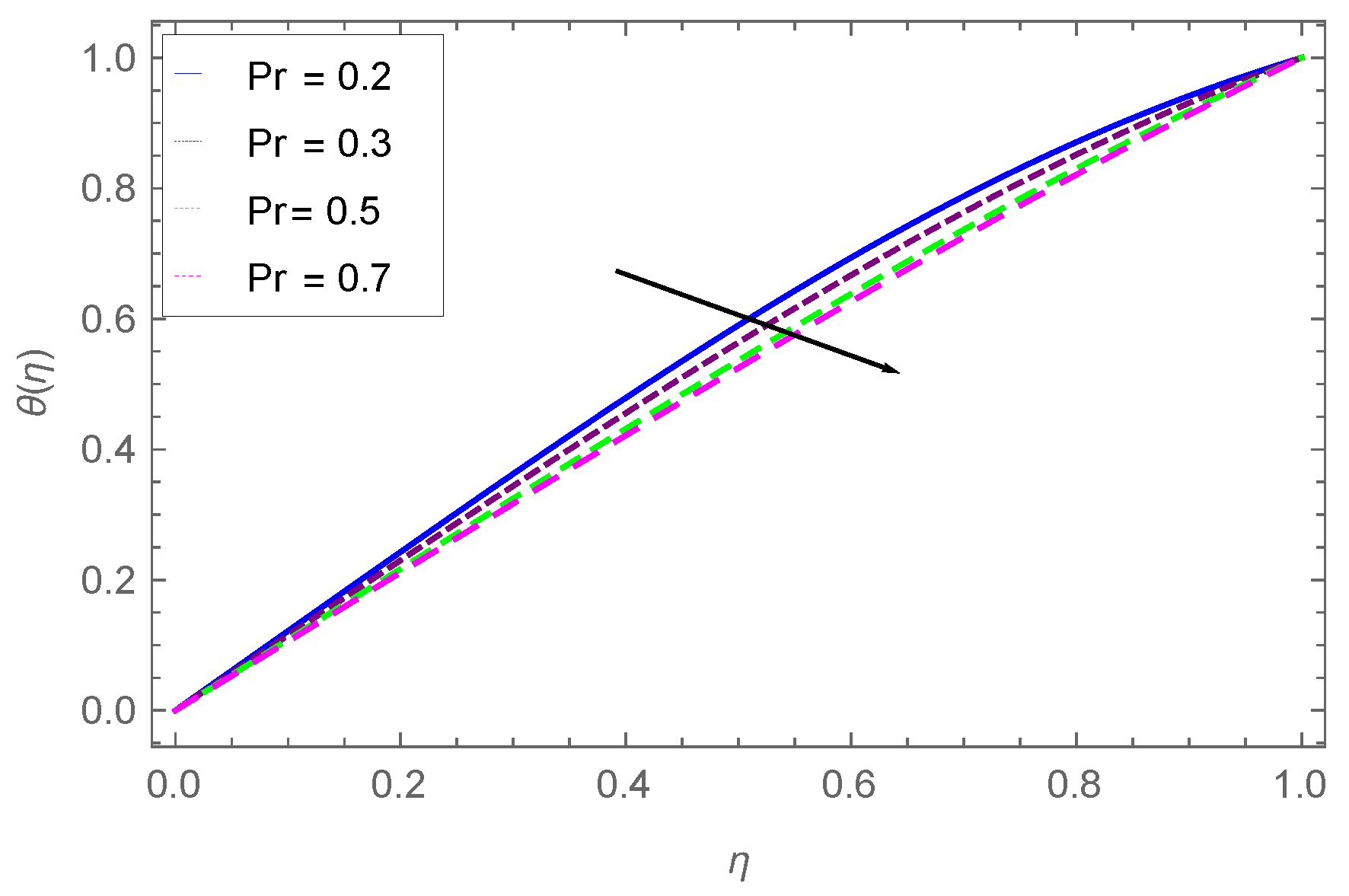
Figure 7 displays the variation in
with changing Prandtl number (
) values. The figure shows a decreasing behavior with higher values of the Prandtl number. The decreasing trend is more significant for the highest value of
only for the intermediate values of
. The higher values of the Prandtl number correspond to less thermal diffusivity, which results in a decline in the fluid temperature. The temperature function
shows the opposite behavior with respect to the variation in
as compared to the variation with respect to
.
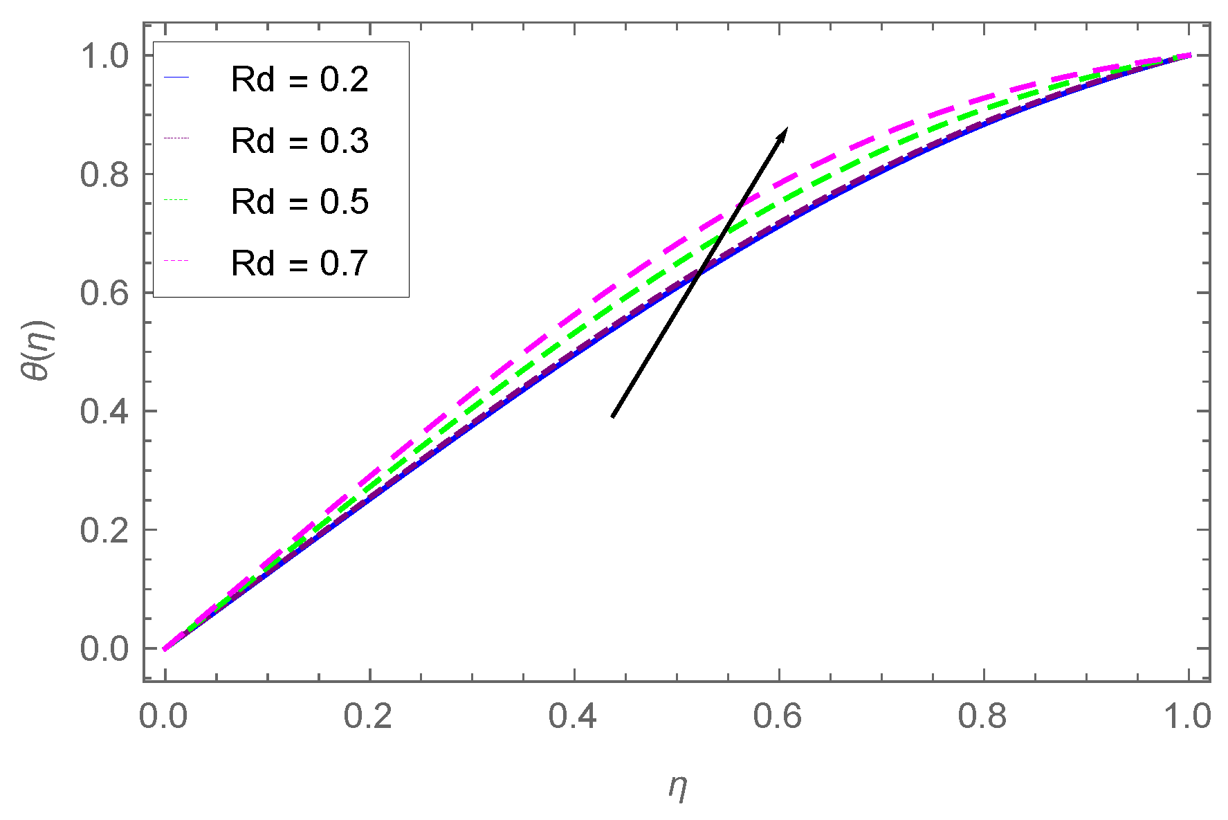
Figure 8 displays the effect of the radiation parameter
on the fluid temperature
. The figure shows that
increases with the higher
values. The increasing trend in the fluid temperature for the higher values of
is evident for the values of
from
to
. Therefore, it is concluded that the presence of thermal radiation augments the fluid temperature.
Figure 9 depicts
for varying scalar parameter
values. It is evident that the temperature field
drops with the changing
values. We see that at
,
increases with a uniform rate up to about
and then decreases beyond it. The spacing between different curves is reduced with increasing
. Furthermore, the
profiles overlap with one another at larger values of
. The increasing
is associated with higher nanoparticle density, which decreases the temperature due to increasing thermal conduction.
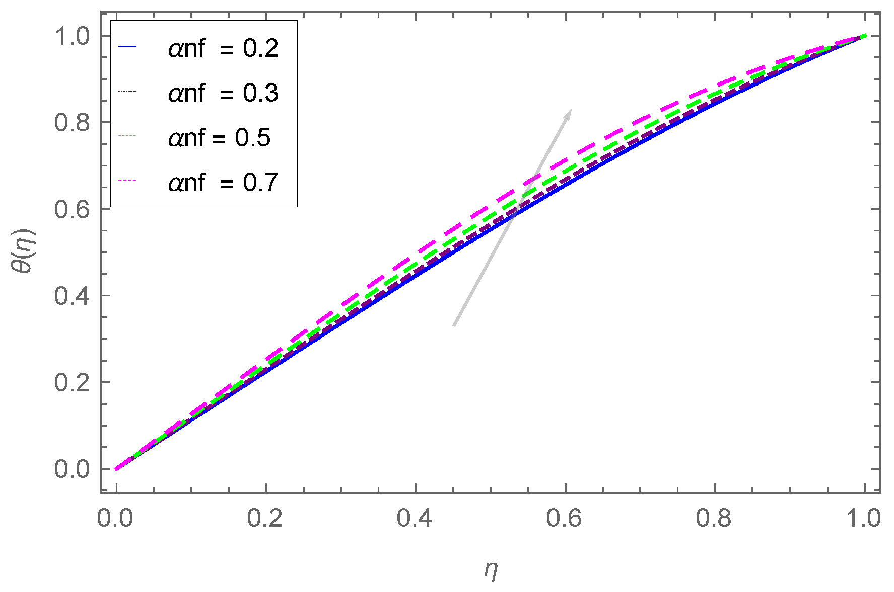
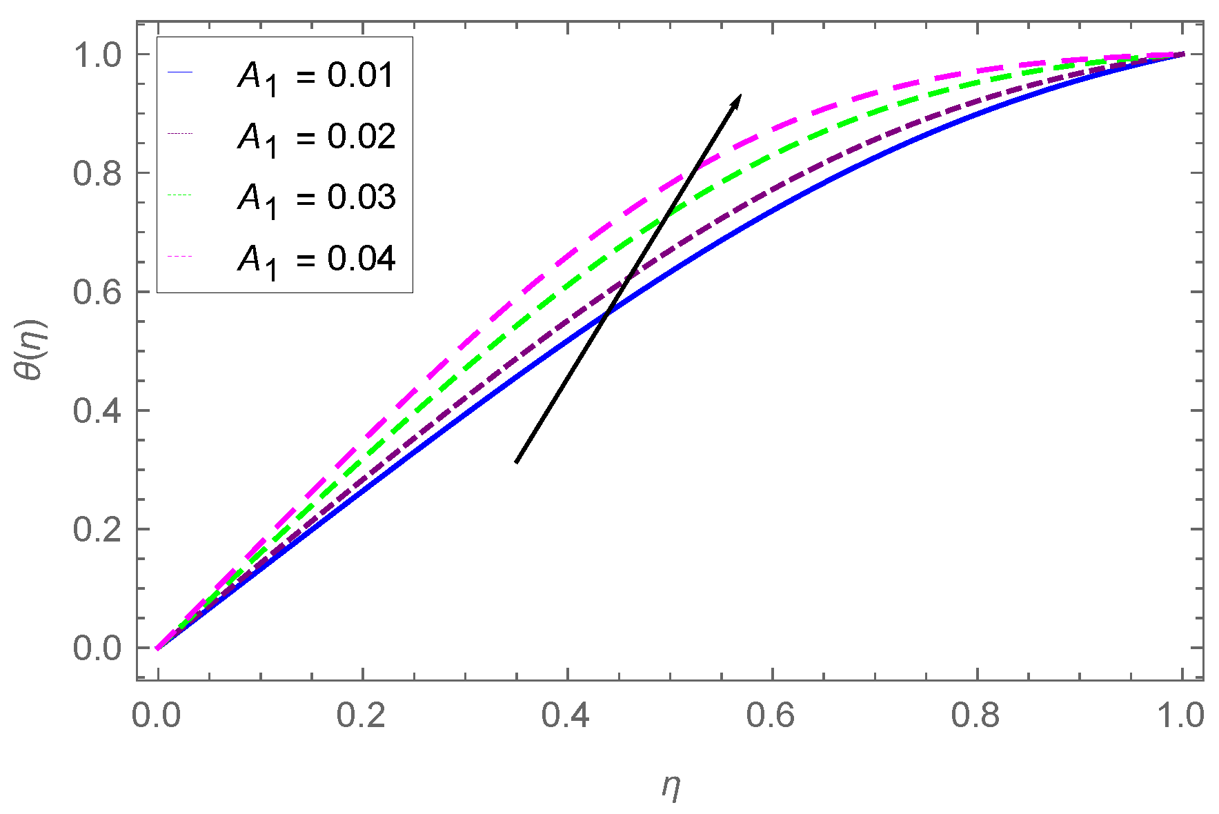
The dependence of the fluid temperature
on
for increasing values of
is shown in
Figure 10. An increasing trend in the temperature is observed at the intermediate values of
for increasing
. Thus, the changing dynamic nanofluid viscosity, which is associated with increasing
, results in an increase in the temperature distribution of the nanofluid.
The dependence of
on
for varying
is displayed in
Figure 11. We observed the same behavior as in the case of
Figure 10. This increase in the temperature with increasing values of
is due to increasing nanofluid-specific heat.
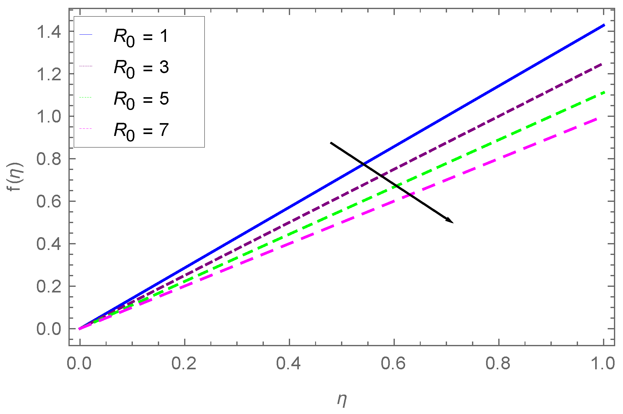
The dependence of
on the rotation parameter (
) is displayed in
Figure 12. The figure shows that
increases with increasing
at fixed
. The velocity profile drops with increasing
. Thus, the increasing rotation rate increases the opposition to the flow in the axial direction, and hence decreases the velocity in that direction. The spacing between different curves is reduced with increasing
.
Figure 13 depicts the variation in
with changing
. It is observed that
shows completely opposite behavior with increasing
, as shown by
in
Figure 12. This means that the changing rotation rate associated with the higher values of
increases
.
The effect of
(couple stress parameter) on
is plotted in
Figure 14. It is observed that the velocity profile changes with higher
values. Thus, the increasing couple stress parameter changes the nanofluid velocity in the axial direction. Near the surface, the viscosity effect is dominant, and in a particular region away from the surface, the higher values of
decrease the viscous effects and, as a result, the velocity profile increases in the axial direction.
The variation in
with changing values of (
) is displayed in
Figure 15. A similar trend is also shown in
Figure 14 for the axial velocity. The couple stress parameter is linked with the viscosity, so increasing the couple stress parameter reduces the viscosity effects and, as a result, the velocity profile increases. On the other hand, far away from the surface where the viscosity effects are negligible, the velocity profile declines with higher values of the couple stress parameter.
The impact of the nanofluid volume fraction parameter on the axial velocity
is displayed in
Figure 16. It is clear from the figure that at intermediate values of the independent variable (
), the velocity profile declines at a rapid rate as compared to the boundary values. Physically, when the nanoparticle volume fraction increases, the mass per unit volume also increases, and as a result, when the nanofluid volume fraction increases from
to
, the axial velocity profile declines.
The impact of the nanoparticle volume fraction parameter
on the draining velocity
in the x-direction is displayed in
Figure 17. A similar trend is displayed in
Figure 16 for the axial velocity. The larger values of the nanoparticle volume fraction reduce the velocity profile, and it is maximum at the intermediate values of
. On the other hand, the nanoparticle volume fraction decreases the boundary layer thickness as well. In conclusion, we can say that the velocity of the ordinary fluid (water in our case) is higher as compared to nanofluids. These results are also reported by Gireesha et al. [
56].
The variation in the thermal boundary layer for various values of the nanoparticle volume fraction is portrayed in
Figure 18. As we have stated earlier, the larger values of the nanoparticle concentration decrease the boundary layer thickness. That is why the larger values of the nanoparticles increase the temperature profile. The variation in the thermal boundary layer is larger at
, when the nanoparticle volume fraction values increase from
to
.
The dependence of the Nusselt number (
) on
for changing values of
is plotted in
Figure 19. The figure shows that for a fixed value of
,
does not change with the variation in the values of
. Furthermore, the plot also shows that by increasing
to larger values,
also increases in approximately equal proportions. Thus, the increasing Pr, which is due to the higher values of momentum diffusivity, augment the convective thermal energy flow of the nanofluid.
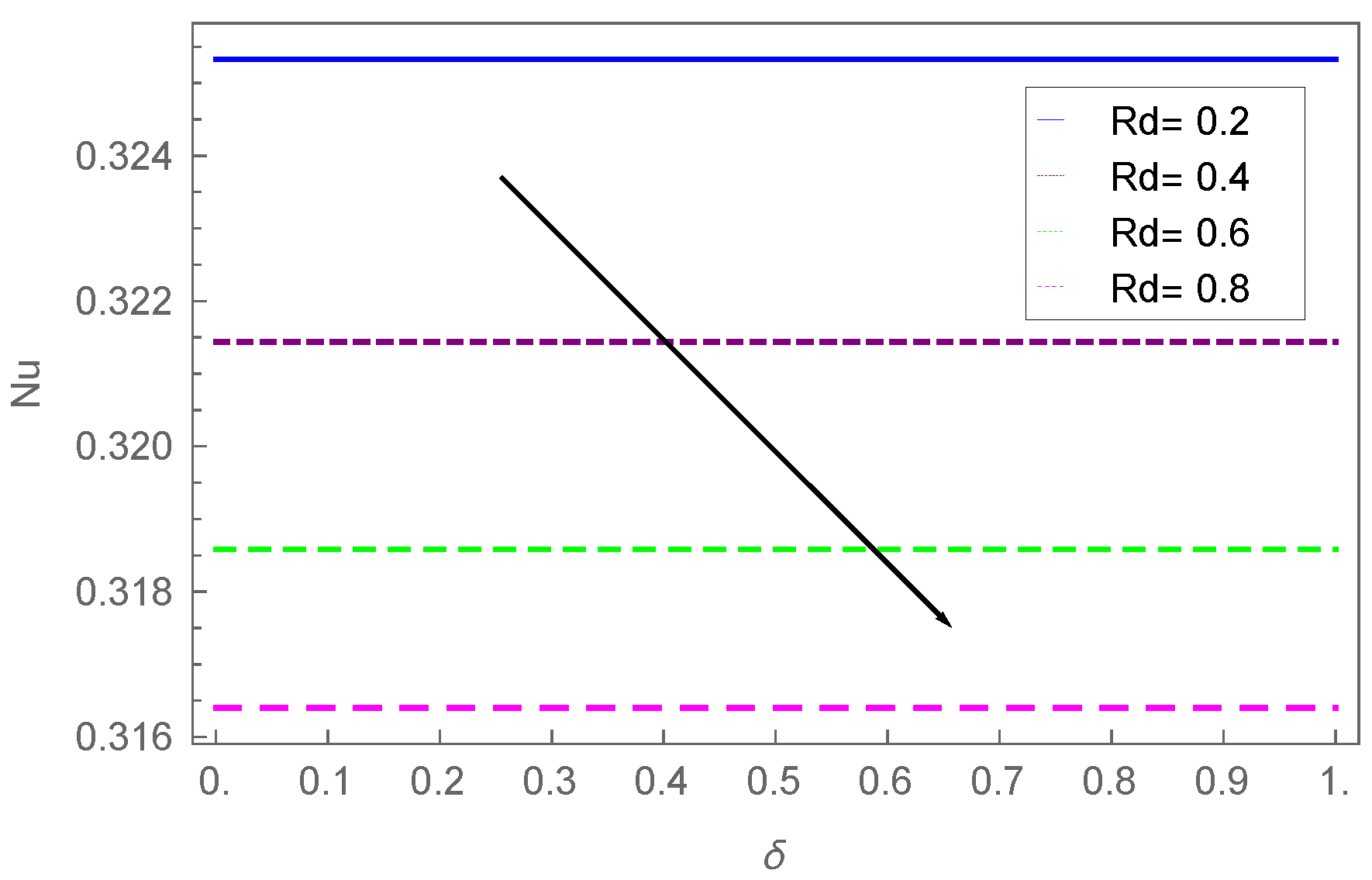
Figure 20 displays the Nusselt number (
) against
for varying radiation parameter (
) values. It is clear that at a fixed value of
,
remains constant when changing the values of
. By increasing
to larger values,
drops to smaller values, maintaining the same constant trend with increasing
. This shows that the changing radiation parameter values decrease the convective thermal energy flow.
6. Discussion of Tables
This section is devoted to the comparison of the present (numerical) and analytical (HAM calculation of the same study) results for the velocity components and temperature function. This comparison is described in
Table 1,
Table 2,
Table 3,
Table 4 and
Table 5. We can see that the HAM and numerical results agree with one another with a good degree of accuracy.
Table 1 shows the comparison for the velocity component
. The value of
changes from
to
, with a step size equal to
. From the table, it is clear that after a few iterations, the numerical results match with HAM results up to four decimal places, as is evident from the absolute error on the rightmost column. The relative difference between the two computations decreases to three decimal places beyond
.
Table 2 shows the comparison of the velocity component
for the two computations. The step size is chosen to be
, whereas
varies from
to
. The HAM and the numerical calculations are in excellent agreement and the absolute error is very small in this case. The maximum relative difference for the two results decreases to six significant figures beyond
. The comparison between analytical and numerical computations for the component
is given in
Table 3. The independent variable
ranges from
to
with a step size equal to
. We see that the numerical and the analytical calculations are in agreement after a few iterations. The absolute error calculation in the right column demonstrates that both results are in agreement up to four significant figures. Similarly, from
Table 4, we note that HAM and numerical calculations are in excellent agreement for
as well. We have compared the results of both procedures (HAM and numerical) for the evaluation of the temperature function (
) in
Table 5. It is evident that there is a very small absolute error between numerical results and HAM calculations. The absolute error for the largest value of the independent variable,
, is
, which is a negligible number. Thus, we can see that the numerical calculations match completely with the analytical (HAM) results.


 ,
, 


