Centralized Energy Prediction in Wireless Sensor Networks Leveraged by Software-Defined Networking

Abstract

Resource Constraints in Wireless Sensor Networks are a key factor in protocols and application design. Furthermore, energy consumption plays an important role in protocols decisions, such as routing metrics. In Software-Defined Networking (SDN)-based networks, the controller is in charge of all control and routing decisions. Using energy as a metric requires such information from the nodes, which would increase packets traffic, impacting the network performance. Previous works have used energy prediction techniques to reduce the number of packets exchanged in traditional distributed routing protocols. We applied this technique in Software-Defined Wireless Sensor Networks (SDWSN). For this, we implemented an energy prediction algorithm for SDWSN using Markov chain. We evaluated its performance executing the prediction on every node and on the SDN controller. Then, we compared their results with the case without prediction. Our results showed that by running the Markov chain on the controller we obtain better prediction and network performance than when running the predictions on every node. Furthermore, we reduced the energy consumption for topologies up to 49 nodes for the case without prediction.

1. Introduction

Wireless sensor networks (WSN) are formed by interconnected nodes with the capacity of sensing, processing, and communicating. Advances in digital electronics, wireless communication, and microelectromechanical systems (MEMS) have enhanced WSN popularity, a technology currently used in a vast number of applications, such as environmental, industrial and health monitoring, tracking and detection, home automation, and security [1]. WSN is also a key technology in the development of the Internet of Things (IoT) [2]. These networks are resource constrained, typically having low processing power, low storage capacity, limited bandwidth, and limited energy. Those restrictions are important to reduce the cost of hardware production but limit the network flexibility, resource reuse, security, and network lifetime.

Kobo et al. [3] state that to solve WSN-inherent problems, including energy and computational constraints, a holistic solution is necessary. Previous works propose integrating WSN with Software-Defined Networking (SDN) as a potential solution to the previously mentioned limitations. The SDN approach decouples the control plane from the data plane, centralizing the routing decisions in the SDN controller [4,5]. The integration of WSN and SDN is referred to in the literature as Software-Defined Wireless Sensor Networks (SDWSN) [6,7,8,9], and results show that SDWSNs perform as well as RPL [9] (IPv6 Routing Protocol for Low-Power and Lossy Networks, RFC 6550).

Routing in WSN considers the resource constraints and the performance demands from applications [10,11]. For example, an energy-aware routing protocol uses energy consumption metrics to extend the network lifetime [12]. In SDN-based networks, the controller is in charge of all routing decisions, and for this reason, it needs information about the network topology and status (i.e., performances metrics), such as energy consumption metrics. To understand the importance of this information in the SDN controller, Oliveira and Margi [12] applied energy-aware route selection to SDWSN. In their proposal, each node reports its remaining energy to the controller every time there is a decrease higher than 1% of the total energy supply. The energy-aware route selection performance was compared to a link quality route selection using the expected transmission count (ETX), a routing metric based on active probing measurements [13]. Their results showed that using the energy-aware route selection increases the network lifetime and reduces the number of route changes. However, this requires that the network devices periodically inform their energy information (i.e., average energy consumption or residual energy) to the SDN controller to maintain the routing metric updated, which increases packets traffic and impacts the network performance.

Several authors proposed mechanisms to reduce the transmissions of these packets. Their main objective is to predict future values of a monitored variable to reduce the frequency of transmissions to update the metric value [14,15,16,17]. For example, Dias et al. [16] implemented autoregressive algorithms in an IoT context to predict sensing measurements, with results depicting a reduction in data transmission and energy consumption. Mini et al. [17] compared Markov chain and time series based node energy consumption prediction algorithms in WSN, and obtained a reduction in the number of messages with energy consumption information for both cases. On the other hand, the prediction requires processing and energy resources that are scarce in WSN nodes.

In this work, we study the benefits and consequences of moving the prediction execution from every WSN node to one centralized node without resource constraints. For this, we decided to implement our proposal using an SDN architecture. Thus, we can use the SDN controller processing power to predict the energy consumption of every node in the network and its communication structure to share the information between the WSN nodes and the controller. Our hypothesis is that by centralizing the prediction we can improve the prediction accuracy and network performance if compared with the case that every node runs the prediction. This is important for two main reasons: (i) improving network performance means improving the delivery rate and decreasing delay of energy information required for control decisions without impacting on other packets traffic, and (ii) in case of missing packets, the controller will be able to predict the missing information. The second point is not possible to solve in the cases without prediction or executing the prediction on every node unless the node retransmits the packet, which means more packets traffic.

Previous works tested Markov chain [18,19] for energy consumption prediction in SDWSNs but, to the best of our knowledge, only our previous work [20] implemented the Markov chain running in the controller to predict the network energy consumption of each node in the network. Here, we extend our previous research by implementing and comparing two strategies: the prediction algorithm runs on all the sensor nodes and the prediction algorithm runs only on the controller node. The metrics we used to compare the performance were prediction accuracy, energy consumption, packets delay, delivery rate, and control packets overhead. Despite being widely used to support prediction in networks, machine learning strategies do not apply to our problem as one could not run the ML prediction algorithm on resource-constrained devices given a large amount of data necessary [21].

Our key findings are that by moving the prediction processing overhead to the SDN controller, we obtain a better prediction accuracy, improved network performance, and reduced energy consumption. However, this approach increases the traffic of packets related to energy consumption information.

The remainder of this paper is organized as follows. Section 2 reviews related works about energy consumption prediction using Markov chain in WSN. Section 3 explains the Markov chain based energy consumption prediction. Section 4 details our energy prediction proposal. Section 5 shows and discusses the experiments and results, and Section 6 concludes the paper.

2. Related Work

In this section, we analyze the literature about energy consumption prediction in WSN using Markov chain models. We emphasize the analysis of works studying energy consumption prediction on SDN-based networks.

Main results presented by the works implementing Markov chain for energy consumption prediction in WSN have shown a reduction of the traffic of packets containing energy information and the energy consumption itself [17,22,23]. Moreover, the energy models used in these works did not include important elements that affect the accuracy, e.g., the sensing module or the processing module energy consumption [24]. More accurate models provide more accurate and precise network lifetime estimation but require more memory and processing resources. Thus, the implementation of accurate energy models in resource-constrained devices is a current challenge.

Recent works propose different strategies to improve energy efficiency and network performance based on the prediction of energy-wise information. In [25], authors propose to predict link quality metric based on an energy density factor using a fuzzy interference system. Then, in [26] authors propose a black widow optimization based algorithm to predict sinks location in mobile WSNs. Their results showed an improvement in energy efficiency; moreover, these works did not address the problem of centralization of energy information and its impact on the network performance.

In traditional WSN networks, it is common that individual nodes run the energy consumption prediction algorithm and inform the result to a central node. The SDN paradigm has open the opportunity to migrate processes from individual nodes to the SDN controller, such as communication channel assignment [27], traffic analysis [28], intrusion detection [29,30], or energy consumption prediction.

In a previous work [20], we implemented a centralized energy consumption prediction for SDWSNs. Similar approaches were implemented by Rahimifar et al. [18] and by Miranda et al. [19]. In [18,20], the SDN controller receives energy consumption information from the nodes in the network; the main difference is that in [18] the nodes do the prediction and send an energy consumption rate to the controller, while in [20] the nodes send to the controller the information required to do the prediction using Markov chain. Unlike the works in [18,20], in [19] the WSN nodes communicate the energy information to a specific sink instead of to the controller. Moreover, they propose a centralized detection as well.

From the results in [18,19,20], we know that the energy prediction strategy can reduce the average energy consumption of the nodes and delay of the packets containing energy information. However, these works do not investigate the impact of their proposals in performance metrics such as control and data packets overhead, delivery rate, and delay. Moreover, the energy models used are not “complete”. According to the works in [31,32], processing and sensing processes represent around $15\%$ of the total consumption. Furthermore, the authors of [24] showed that the consumption by states transitions could have a significant part in the final result. Thus, accurate energy consumption models should consider processing, sensing, communication and transitions energy consumption.

From previous works, we noticed that (i) energy prediction proposals for WSN using Markov chain are based on energy models that omit the processing and/or sensing energy consumption, (ii) the energy consumption prediction proposals have been tested through simulations but there is a lack of experiments in real devices, and (iii) the centralized prediction works based on Markov chain have shown promising results, but there are not enough results to measure the impact of its implementation in the network performance.

In this work, we addressed these gaps in the literature by implementing a centralized Markov chain-based energy consumption prediction using an energy model that considers processing, sensing, communication, and transitions consumption. Our objective is to propose an energy consumption prediction algorithm leveraged by SDN that is accurate and lightweight in terms of processing and communication resources. We evaluated the performances of our proposal through simulations, emulating sky motes, and experiments on real devices using TelosB motes. To evaluate the impact on the network performance, we measured the delivery rate, delay, packets overhead, and energy consumption.

3. Energy Consumption Prediction

This section has three main parts: first, we explain the basics of Markov chain and how we apply it to predict energy consumption in WSN; second, we propose an energy consumption model for WSN; and third, we explain the integration of the energy consumption model and the Markov chain for energy consumption prediction.

3.1. Markov Chain

A Markov chain is a stochastic process commonly used to model dynamic systems, such as computer behavior [33]. A Markov chain is composed of a set of states and the transition probabilities from one state to another, where the probability of the next state depends only on the current state (Markov property).

The Markov chain is represented by a probability matrix or by a transitions diagram, among other representations. In the case of using a matrix, the entries are the probabilities of a transition from one state to another. For example, for a probability matrix P, the element $P_{12}$ is the probability of a transition from the state “1” to the state “2”. Assuming $X_0$ is the initial state-space distribution and $X_1$ is the state-space distribution in the next time-step, $X_1=X_{0}P$. Then, $X_2=X_{1}P=X_{0}PP$, hence $X_n=X_0{P}^n$, where $P^n$ is the probability matrix to the power of n.

Then, assume $E_R$ represents the state’s energy consumption prediction. To calculate $E_R$, we need to predict the number of visits to each state for the time we want to predict the energy consumption. The number of visits to state j starting from state i for n steps is $N_j={\sum }_{t=1}^n{P}_{ij}^t$, where $P_{ij}^t$ is the probability of going from state i to state j to the power of t. Moreover, the number of visits for all states is calculated as shown in Equation (1), where $P^t$ is the probability matrix to the power of t.

$$N=\sum _{t=1}^n{P}^t$$

(1)

Then, the energy consumption by all the states $E_R$ is calculated as shown in Equation (2), where $E_s^T$ is a vector that contains the average energy consumption of each state transpose.

$$E_R=X_{0}N{E}_s^T$$

(2)

Substituting $E_S^T$ in Equation (2) by a matrix $K_s$ that represents the cost of one transition, we predict the energy consumption for all transitions during n steps. We obtain $K_s$ calculating the element-wise product (∘) of probability matrix P and transitions cost matrix B, as shown in Equation (3). Then, $E_B$ in Equation (4) is the energy consumption only by transitions after n steps, where e is a vector with all the entries 1.

$$K_s=P\circ B$$

(3)

$$E_B=X_{0}N\left(K_s{e}^T\right)$$

(4)

Therefore, the total energy consumption predicted for the next n steps is

$$E_{total}=E_R+E_B$$

(5)

3.2. Energy Consumption Model

The energy consumption prediction using Markov chain requires that the energy consumption of each state in the set is known. Furthermore, we need a mechanism to evaluate the prediction accuracy of our proposal. To fulfill both requirements, we propose an energy consumption model that considers processing, sensing, communication, and transitions consumption.

3.2.1. Sensing Module

The sensing modules operate mostly using two states: active and sleep mode. In the active state, the module takes the measurement and transmits it to the MCU. In the sleep mode, it turns off most of its submodules to reduce the energy consumption and remains waiting for a signal to acquire the next measurement. Considering both states and the transitions between them, the sensing module energy consumption (represented as $E_{Sen}$) is calculated using Equation (6). The term $E_{sen-act}$ represents the active state, $E_{sen-sleep}$ the sleep mode, $E_{sen-on}$ the turning on transition, and $E_{sen-off}$ the turning off transition.

$$E_{Sen}=E_{sen-act}+E_{sen-sleep}+E_{sen-on}+E_{sen-off}$$

(6)

To calculate the energy consumption for a certain period, the terms $E_{sen-act}$ and $E_{sen-sleep}$ are expressed in terms of power consumption and time. Then, we calculate the transitions energy consumption by multiplying the average transition energy consumption by the total transitions counted in this period of time. Thus, $E_{Sen}$ is expressed as shown in Equation (7), where $P_{sen-act}$ and $P_{sen-sleep}$ are the active and sleep mode states average power consumption; $T_{sen-act}$ and $T_{sen-sleep}$ are the time spent on the active and sleep mode states; $e_{sen-on}$ and $e_{sen-off}$ are the average energy consumption of one turning on and turning off transitions; and $N_{on}$ and $N_{off}$ are the number of transitions.

$$\begin{array}{c}{E}_{Sen}=P_{sen-act}{T}_{sen-act}+P_{sen-sleep}{T}_{sen-sleep}+N_{on}{e}_{sen-on}+N_{off}{e}_{sen-off}\end{array}$$

(7)

3.2.2. Processing Domain

The processing module’s energy consumption model is based on the work in [31], which considers at least three states: active, idle, and sleep. For our proposal, we change the sleep state for power-saving states. This means more than one state is meant to reduce energy consumption. Thus, the processing energy consumption $E_{CPU}$ for a certain period is calculated as shown in Equation (8).

$$\begin{array}{c}{E}_{CPU}=P_{cpu-act}{T}_{cpu-act}+P_{cpu-id}{T}_{cpu-id}+\sum _{s=1}^S{P}_{\{pp,s\}}{T}_{\{pp,s\}}+\sum _{g=1}^G{N}_g{P}_{\{cput,g\}}\end{array}$$

(8)

The terms $P_{cpu-act}$, $P_{cpu-id}$, and $P_{\{pp,s\}}$ are the active, idle, and power-saving states average power consumption, respectively. The terms $T_{cpu-act}$, $T_{cpu-id}$, and $T_{\{pp,s\}}$ are the time spent in the active, idle, and power-saving states, respectively. The terms $N_g$ and $P_{\{cput,g\}}$ are the number of g transitions and their average power consumption. The transitions energy consumption is calculated by multiplying the number of transitions and their average energy consumption.

3.2.3. Communication Domain

Two approaches are used to calculate the energy consumption in the communication module. One approach is based on the number of bits transmitted and received [32,34]. The other approach is based on operation states, measuring the time spent on each state to estimate the total energy consumption [31,35], as explained for the processing and sensing modules. We chose to use the operation states approach to give homogeneity to the model.

Figure 1 depicts a simplified block diagram for a WSN communication module, based on four IEEE 802.15.4-compliant radios modules (CC2420 [36], CC1120 [37], MRF24J40 [38], and CC2520 [39]). Then, based on the simplified block diagram, four states were defined: transmitting, receiving, idle, and sleeping. When the module is in the transmitting state, the transmitter circuitry and the control logic block are active. In the receiving state, the receiver circuitry and control logic block are active. When the receiver and transmitter circuitry are turned off and the control logic block is turned on, the module is in the idle state. Last, when the receiver and transmitter circuitry are turned off and the control logic block is in the sleeping mode, the module is in the sleeping state.

Equation (9) express the energy consumption for a certain period of time. The terms $P_{Tx}$, $P_{Rx}$, $P_{com-id}$, and $P_{com-sl}$ are the transmitting, receiving, idle, and sleeping states average power consumption. The terms $T_{Tx}$, $T_{Rx}$, $T_{com-id}$, and $T_{com-sl}$ are the time spent on transmitting, receiving, idle, and sleeping states. The terms $N_q$ and $P_{\{ct,q\}}$ are the number of q transitions and its average power consumption, respectively.

$$\begin{array}{c}{E}_{Com}=P_{Tx}{T}_{Tx}+P_{Rx}{T}_{Rx}+P_{com-id}{T}_{com-id}+P_{com-sl}{T}_{com-sl}+\sum _{q=1}^Q{N}_q{P}_{\{ct,q\}}\end{array}$$

(9)

3.3. Energy Consumption Prediction Implementation

As our proposal is for WSN, we decided to implement our energy consumption model on TelosB motes, an IEEE 802.15.4-compliant platform with an MSP430 microprocessor and 48 kB of flash memory. We modeled the TelosB mote energy consumption considering the device would run a temperature monitoring application, considering that the whole WSN was programmed using Contiki-3.0 [40]. Next, we describe the states of each module.

The temperature sensor of the TelosB is a Sensirion STH11 and it operates in two states: active and sleep. Regarding the processing energy consumption, Contiki avoids staying idle and it supports only two low-power modes: LPM1 and LPM3. Using the default configuration, the microprocessor never enters in LPM3 state. Thus, the processing module operates in two states: active and LPM1. The communication module behavior is defined by the CC2420 Contiki implementation. Contiki uses a radio duty cycle mechanism named ContikiMAC [41]. This mechanism uses a power-aware wake-up mechanism with a set of timing constraints aiming to keep the transceiver turned off as long as possible. An important issue is that using ContikiMAC, the communication module does not enter in the idle state. Furthermore, whenever ContikiMAC turns off the radio, the frequency synthesizer is disabled, which means the module is in the power down state. Based on these characteristics, the communication module operates in three states: transmitting, receiving, and power down.

Based on the TelosB energy consumption characteristics, we defined five states for the Markov chain: Sensing, Processing, LPM1, Transmitting, and Receiving. Each state is composed of three substates, one for each module.

Table 1. Set of states of the Markov chain.

State	Domain
	Sensing	Processing	Communication
Sensing	active	active	sleeping
Processing	sleeping	active	sleeping
LPM1	sleeping	LPM1	sleeping
Transmitting	sleeping	active	transmitting
Receiving	sleeping	LPM1	receiving

describes the configuration of each Markov chain state.

The probability matrix is constructed after a training period where each node monitors its transitions. Each node constructs a transitions matrix to organize the number of transitions between states and a transitions vector to store the total of transitions of each state. Then, dividing each row of the transitions matrix by the total number of transitions, as shown in Equation (10), we obtained the probability matrix. Then, we can calculate Equations (2) and (4) to obtain the energy consumption prediction. Note that P depends on the node’s behavior, which means that it can change every time it is calculated, according to the transitions (a and v) counted.

$$P=\left(\begin{array}{ccccc}{a}_{11}/v_1& a_{12}/v_1& a_{13}/v_1& a_{14}/v_1& a_{15}/v_1\\ a_{21}/v_2& a_{22}/v_2& a_{23}/v_2& a_{24}/v_2& a_{25}/v_2\\ a_{31}/v_3& a_{32}/v_3& a_{33}/v_3& a_{34}/v_3& a_{35}/v_3\\ a_{41}/v_4& a_{42}/v_4& a_{43}/v_4& a_{44}/v_4& a_{45}/v_4\\ a_{51}/v_5& a_{52}/v_5& a_{53}/v_5& a_{54}/v_5& a_{55}/v_5\end{array}\right)$$

(10)

4. Centralized Energy Consumption Prediction

According to the literature review, previous works implementing centralized energy consumption prediction in WSN maintain the prediction processing overhead on the sensor nodes. The WSN nodes monitor their behavior, execute the prediction algorithm, estimate an energy consumption rate, and send this information to a sink or controller. We propose to move most of the processing required for the prediction to the SDN controller, assuming that the SDN controller does not have energy, processing power, or memory space constraints. In this manner, the WSN nodes monitor their behavior and the controller executes the prediction algorithm.

In detail, the WSN nodes execute a training period to calculate their probability matrix. Each node has to register all the transitions and order them in a matrix, just as explained in Section 3.3. When the training process ends, the node calculates the probability matrix and the energy spent up to this moment; then, it sends this information to the SDN controller. The SDN controller creates an energy profile for each node. This profile contains the probability matrix and an energy consumption time series, constructed from the information sent by the WSN nodes and the prediction results.

The SDN controller executes the prediction algorithm (Algorithm 1) to calculate the energy consumption for the next n steps. Then, the SDN controller informs the prediction value obtained to the respective WSN node. In this manner, after n steps the node can calculate the prediction error by comparing the prediction and the energy consumption obtained through the energy model. If the error is above a threshold previously defined, the WSN node initiates a new training period to update the energy information in the energy profile in the SDN controller. On the other hand, if the error is below the threshold, the SDN controller continues the time series construction using the value predicted.

Algorithm 1 Markov chain running on the controller

1: n: number of steps 2: $prediction$: energy consumption prediction for n steps 3: $error$: prediction error 4: $threshold$: maximum error accepted 5: $p\_matrix$: transitions matrix 6: $s\_consumption\left(n\right)$: energy consumption prediction during n steps for states 7: $t\_consumption\left(n\right)$: energy consumption prediction during n steps for transitions 8: ⎯⎯⎯⎯⎯⎯⎯⎯⎯⎯⎯⎯⎯⎯⎯⎯⎯⎯⎯⎯⎯⎯⎯⎯⎯⎯⎯⎯⎯⎯⎯⎯⎯⎯⎯⎯⎯⎯⎯ 9: Running on WSN nodes 10: launch the training 11: wait the training period ends 12: calculate $p\_matrix$ 13: send $p\_matrix$ to the controller 14: while true do 15:   wait n steps 16:   calculate energy consumption 17:   calculate error(energy consumption, last prediction) 18:   if $error$ > $threshold$ then 19:    obtain a new $p\_matrix$ 20:    send new $p\_matrix$ to controller 21:   end if 22: end while 23: ⎯⎯⎯⎯⎯⎯⎯⎯⎯⎯⎯⎯⎯⎯⎯⎯⎯⎯⎯⎯⎯⎯⎯⎯⎯⎯⎯⎯⎯⎯⎯⎯⎯⎯⎯⎯⎯⎯⎯ 24: Running on the SDN controller: 25: wait for WSN information 26: functionprediction ($p\_matrix,n$) 27:   calculate $s\_consumption\left(n\right)$ and $t\_consumption\left(n\right)$ 28:   prediction=$s\_consumption+t\_consumption$ 29:   update time series 30:   send $prediction$ to sensor nodes 31: end function

Implementation

The implementation was conducted using Contiki-3.0 [40], a widely used open-source operating system for WSN, and IT-SDN version 0.4 [9,42] (Available at http://www.larc.usp.br/users/cbmargi/www/it-sdn/, last time accessed 12 August 2021). IT-SDN is an open-source SDWSN framework implemented in our group, with results showing that its performance is similar to RPL for topologies up to 289 nodes.

Previous works used time steps of 1000 ms [17] and 100 ms [43]. Moreover, we decided to use a time step of 1 ms to obtain a more accurate probability matrix. For example, ContikiMAC [41] channel checking takes $0.884$ ms plus the radio turning on and turning off time. Thus, time steps of 1000 ms and 100 ms lose information in our evaluation environment.

The communication between sensor nodes and the controller was implemented using the IT-SDN communication stack. IT-SDN [9,42] is an SDWSN framework composed of three communication protocols: the Southbound protocol, the Neighbor Discovery protocol, and the Controller Discovery protocol. The Southbound protocol defines the message formats for communication between the WSN and the controller. The WSN nodes use the Controller Discovery protocol to find a route to the controller and the Neighbor Discovery protocol to collect neighborhood information. The controller uses the neighbor information to define the routes according to the policies programmed. Then these routes are configured in the WSN nodes.

The Southbound protocol has six packet types: flow request, flow setup, flow ID register, acknowledgment, neighbor report, and data packet. Moreover, we created two more packets to address energy and prediction information communication: one packet exclusively to send energy information (i.e., from sensor nodes to the controller), and another packet exclusively to send the controller’s reply (i.e., from the controller to sensor nodes). The energy information packets are routed using a flow identifier and the reply packets are source-routed from the controller.

All the energy information packets contain a byte specific for prediction mechanism identification. Thus, in the case of having more than one prediction algorithm, the receiver will know how to process the packet. For example, running the prediction on the WSN nodes and running the prediction on the SDN controller. Each case requires different information to be shared, thus using this identifier we inform which one we are implementing. Furthermore, using this identifier we are able to mix both approaches.

Table 2. Energy information packets’ sizes.

Energy Information
Approach	Packet size (B)
Running on the controller	89
Running on the WSN node	15
Controller reply
Running on the controller	12 + 2 × hops

shows packets’ sizes in bytes for both cases.

5. Experiments and Results

In this section, we describe the experiments we used to measure the performance of our energy consumption model and our centralized energy consumption prediction proposal. Then, we analyze and discuss the results obtained.

5.1. Energy Consumption Model Accuracy

The energy consumption model accuracy was evaluated using an N6705C DC power analyzer from Keysight. First, we measured the states and transitions average energy consumption using the power analyzer. Then, we deployed a network as shown in Figure 2 to obtain the energy consumption estimation from one node in an SDWSN and measure its energy consumption with the N6705C at the same time. The controller software runs on a desktop computer Intel Core i5 CPU 750 and 8 GB of memory RAM. All the nodes in the WSN are TelosB motes, including the gateway used to communicate the WSN and the SDN controller. Figure 3a depicts the connection to collect energy consumption measurements using the N6705C equipment and Figure 3b depicts the connection between the SDN controller and the WSN gateway.

We compared the node estimation and the N6705C measurement to calculate the energy consumption model accuracy. During the testing, all the sensor nodes send temperature measurements to the sink and energy consumption measurements to the controller every 20 s. The experiment was replicated ten times, taking ten energy consumption measurements per time. We obtained an average error of $4.98\%$ and a confidence interval of $1.53\%$ using a significance level of $0.05$.

5.2. Prediction Mechanisms Performance Evaluation

The energy consumption prediction proposal performance was evaluated from simulations using COOJA [44] and emulating sky motes, which is a TelosB equivalent available in COOJA simulator. We also executed experiments running the prediction algorithm in the WSN nodes, such as proposed by Rahimifar et al. [18], which for the best of our knowledge, it is the most recent work about energy consumption prediction using Markov chain in SDWSN.

Both approaches were simulated using multihop grid topologies from 16 nodes to 81 nodes, including one controller node and one sink node. We also simulated the scenario without prediction to use it as a baseline. In this case, all WSN nodes send their energy consumption to the SDN controller every 60 s. In parallel, we run a temperature monitoring application where every node sends a temperature sample (2 bytes message) every 60 s as well. Furthermore, all nodes wait 60 s plus a random value between 0 and 60 s before initializing the prediction algorithm and the temperature application. We use the random value to prevent all nodes from transmitting energy and temperature packets at the same time, which would create packets collisions.

The metrics to evaluate the energy consumption prediction proposals include prediction performance and network performance metrics. These metrics are prediction accuracy, total delay, total delivery rate, packets overhead, and energy consumption. The total delay is the average time the packets spent to reach the destination. The prediction accuracy is evaluated in two ways: prediction error and valid predictions rate. The prediction error is the average error of all the predictions during the test. The valid predictions rate is the number of predictions with an error lower than $5\%$ divided by the total predictions performed. We chose $5\%$ based on the average estimation error we obtained using our energy consumption model (Section 5.1). The total delivery rate is calculated by dividing the number of packets successfully received by the number of packets sent. The packets overhead is quantified as the number of packets per minute. The energy consumption is the average energy consumption per minute of all nodes, excluding the sink node and the controller node.

The total delay, total delivery, and overhead metrics are classified by type of packet. Control packets are those related to the IT-SDN control plane, data packets are the application packets sent to the sink, and energy packets are the packets related to the prediction mechanisms and energy information. The graphics in this section show the average results calculated among replications.

Table 3. Abbreviations for the schemes simulated.

Abbreviation	Scheme
No-Prediction	Without prediction
Markov-Node	Markov chain running in the sensor node
Markov-PC	Markov chain running in the controller

shows the abbreviations used for each scheme, and

Table 4. Simulation parameters.

Simulation Parameters
Topology	Square grid
Number of nodes	16, 25, 36, 49, 64, 81
Number of sinks	1
Data traffic rate	1 packet every 60 s
Data payload size	2 bytes
ContikiMAC channel check rate	8 Hz
Radio medium	Unit disk graph medium
Distance between nodes	50 m
Transmission range	55 m
IT-SDN parameters
Neighbor discovery protocol	Collect-based
Link metric	ETX
Controller discovery protocol	none
Route calculation algorithm	Dijkstra
Route recalculation threshold	$20\%$
Flow table size	15 entries

and

Table 5. Energy consumption parameters.

Energy Consumption Parameters
Transmission current consumption	20.3 mA
Receiving current consumption	18.75 mA
Processing current consumption	2.21 mA
Sleeping mode current consumption	0.67 mA
temperature sensor current consumption	2.3 mA
Operation voltage	3 V

summarize the simulation and energy consumption parameters, respectively.

Table 6. Transitions’ energy consumption ($\mathsf{\mu }$J).

	Sensing	Processing	LPM1	Transmitting	Receiving
Sensing	0	0	0	0	0
Processing	75.6	0	1.35	5.94	0
LPM1	75.6	1.35	0	0	7.38
Transmitting	0	10.8	0	0	0
Receiving	0	21.6	0	0	0

represents the cost per transitions in microjoules, i.e., matrix B in Equation (3). The cases with cost zero are transitions that never occurred or that we were not able to measure with our equipment. Last, according to our tests, the initial state is always Processing. Thus, the initial vector $X_0=\begin{array}{ccccc}[0& 1& 0& 0& 0]\end{array}$.

Results Analysis

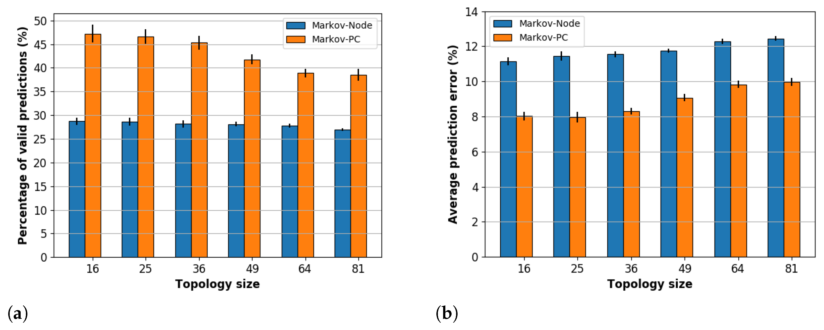
Figure 4a depicts the percentage of valid predictions and Figure 4b depicts the average prediction error metric. The Markov-PC scheme obtained the highest percentage of valid predictions and the lowest prediction error, which means it is the most effective to reduce energy packets updates. Moreover, we observed that the topology size has more impact on the Markov-PC scheme than on the Markov-Node scheme. In terms of percentage of valid predictions, the average results in the Markov-scheme decrease $8.68\%$, from 16 nodes to 81 nodes, while for the Markov-Node scheme the decrease is $1.76\%$.

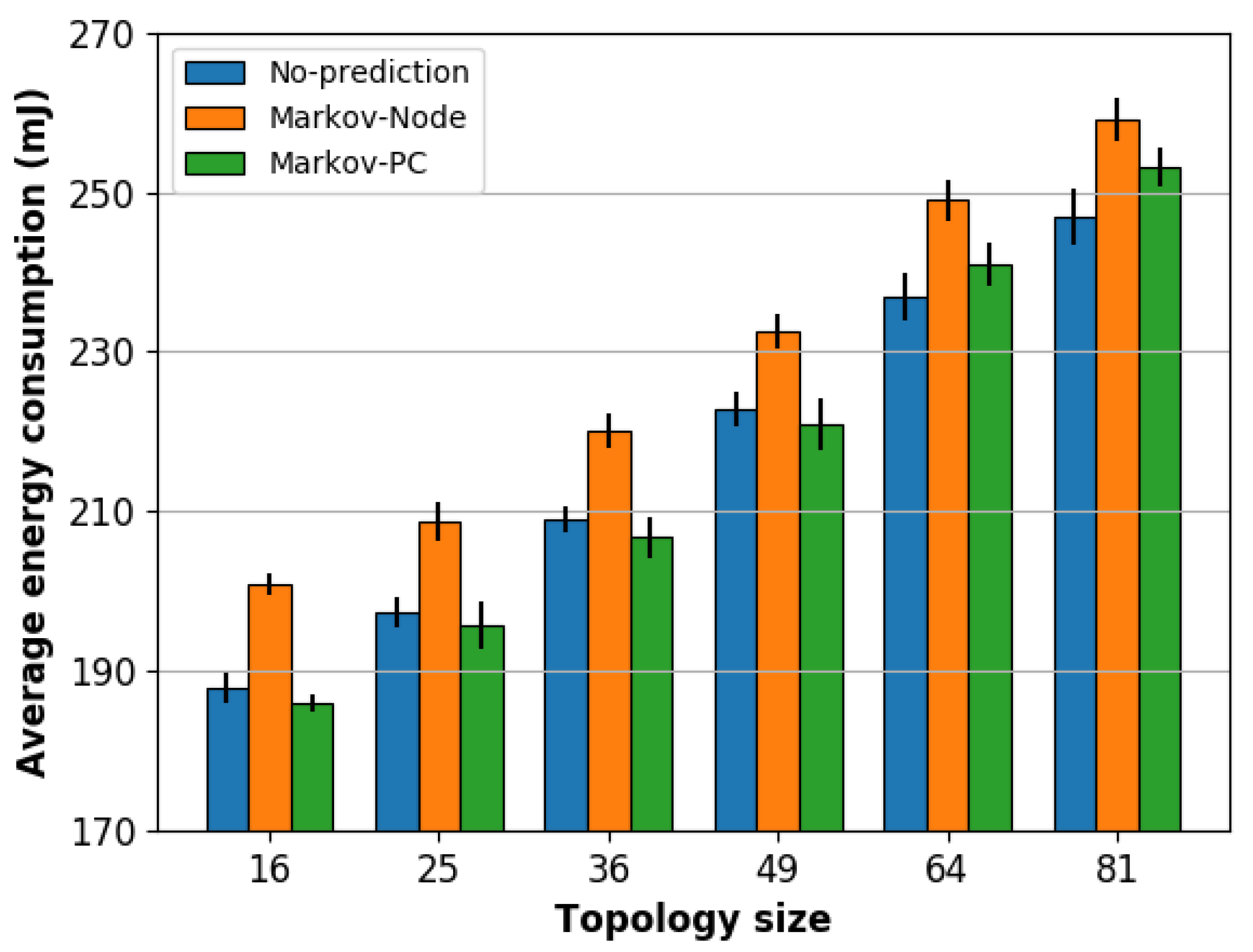
Figure 5 depicts the average energy consumption including the scenario without prediction. Comparing both Markov chain schemes with the No-Prediction scheme, the Markov-PC scheme reduces the average energy consumption of the networks with sizes from 16 to 49 nodes, whereas the Markov-Node scheme increases the average energy consumption for all sizes. This means that the Markov-Node scheme energy consumption trade-off is not positive: it spends more energy than the amount it is able to save. On the other hand, the Markov-PC scheme, the one with the better prediction performance, saves approximately 1% of energy consumption in the topologies between 16 and 49 nodes but increases this metric 1% for 64 nodes and 5% for 81 nodes. If we go back to the percentage of valid predictions in Figure 4a and compare those results with the energy consumption results for Markov-PC scheme, we can say that it is necessary over 40% of valid predictions to save energy.

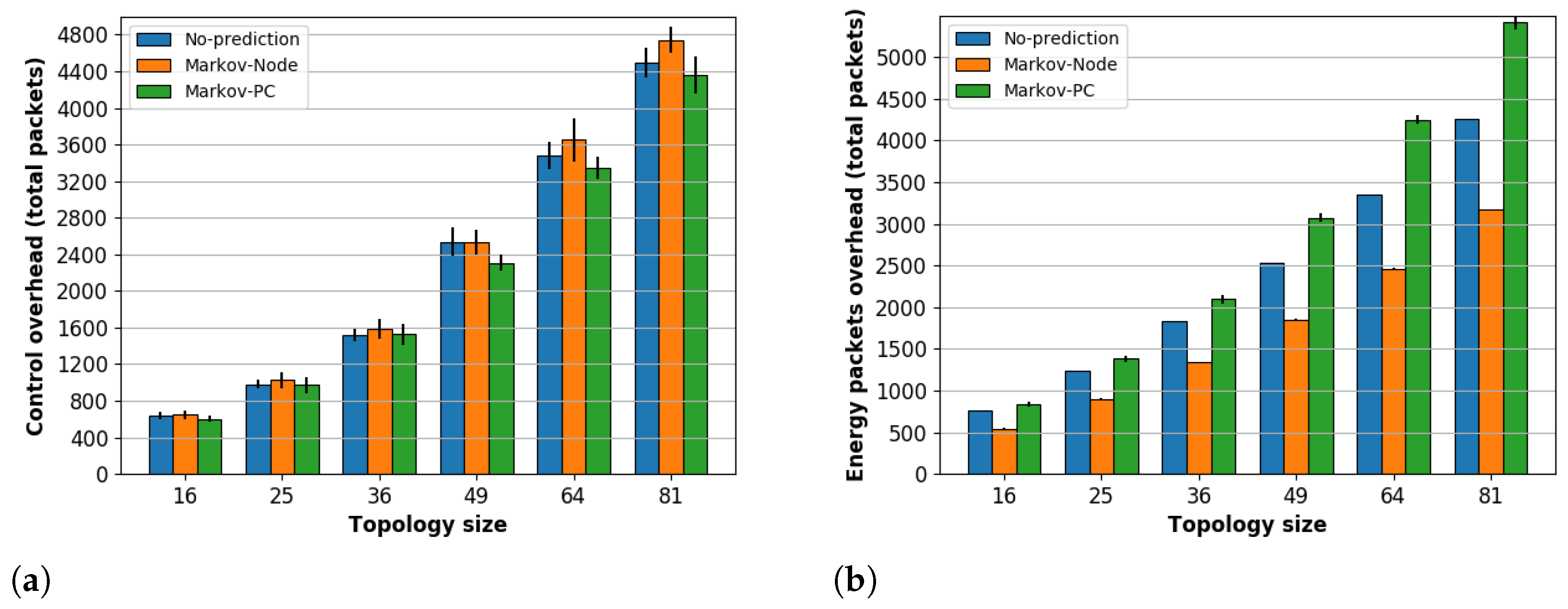
Figure 6a,b depicts the control and energy packets overhead, respectively. Regarding control packets overhead, the results show similar values for all the schemes in topologies from 16 to 36 nodes. This means that the prediction schemes implementation do not increase the control overhead for small networks. Moreover, we observed that the Markov-PC reduces the control overhead in around $3\%$ and $9\%$ for 49, 64, and 81 nodes. On the other hand, the Markov-Node scheme increases the control overhead between $4.9\%$ and $5.4\%$ for topologies with 64 and 81 nodes. This increase is related to the control packets delivery rate, which is analyzed further below.

Then, the results in Figure 6b show that the Markov-Node scheme reduces the energy packets traffic while the Markov-PC scheme increases it. Even though the Markov-PC scheme has a lower prediction error and a higher percentage of valid predictions than the Markov-Node scheme, the increase is because in the Markov-PC scheme the controller replies every energy information update with the energy consumption prediction result, but in the Markov-Node scheme this is not necessary. This means that using the Markov-PC we need $50\%$ or more valid predictions to at least equal the No-Prediction scheme. On the other hand, around $27\%$ of valid predictions (Figure 4a) in the Markov-Node scheme are enough to reduce up to $25\%$ of the energy packets traffic.

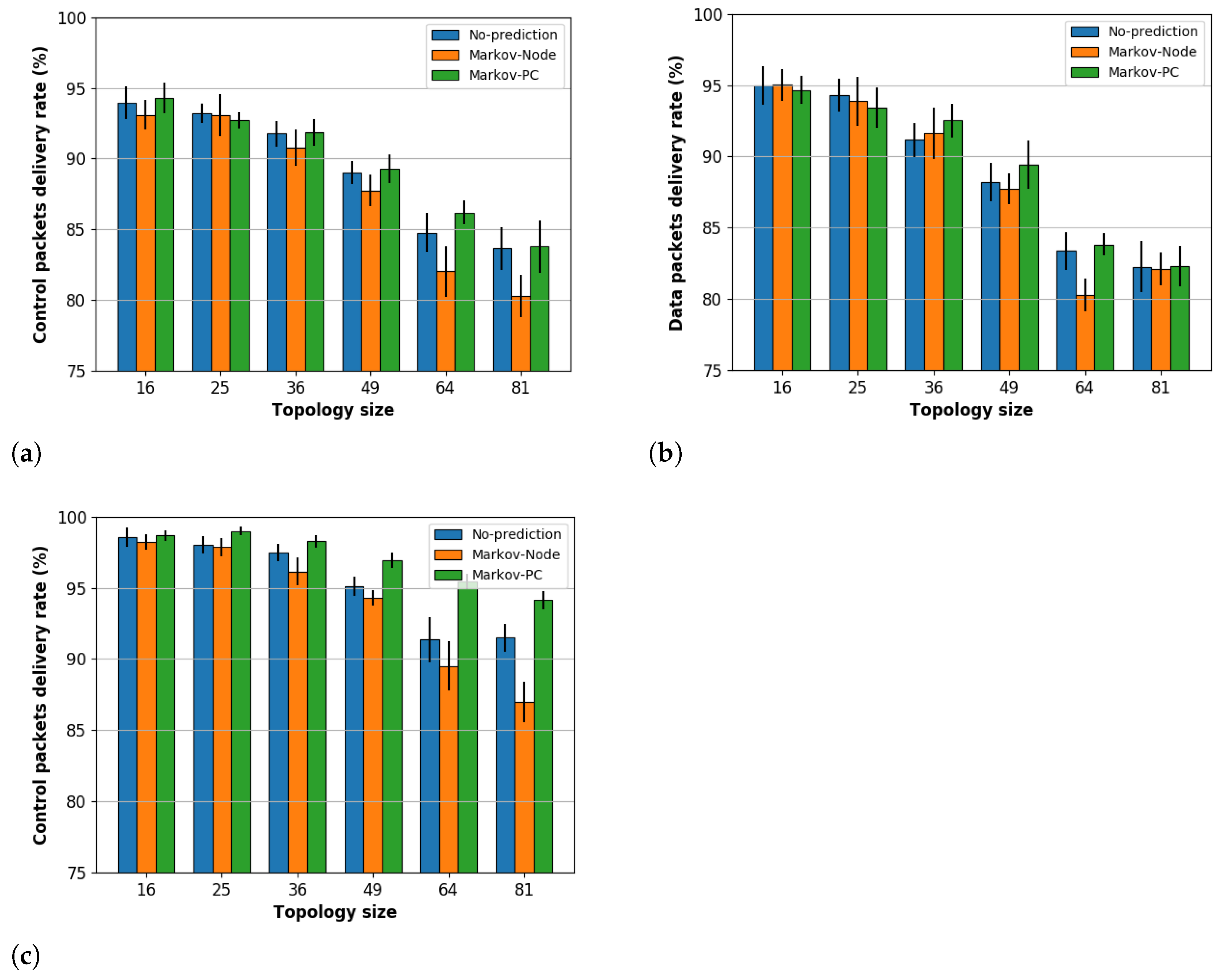
Figure 7a–c depicts the delivery rate for control, data, and energy packets, respectively. From those figures, we observed that the Markov-PC scheme equals or improves the delivery rate with respect to the No-Prediction scheme results. For example, in the case of the energy packets delivery rate, the result for the Markov-PC are between $1.8\%$ and $4.4\%$ over the No-Predictions scheme.

On the other hand, using the Markov-Node scheme the delivery rate is below the No-Prediction scheme results in most cases. This is interesting since the Markov-Node scheme obtained the lowest energy packets overhead, with up to $40\%$ less than the Markov-PC scheme. To understand this, we have to remember that in WSNs all packets share the same band and channel in some cases. Despite the Markov-Node obtained the lowest energy packets overhead, it also obtained the highest control packets overhead, which can affect the energy packets delivery rate. Furthermore, in the Markov-Node scheme all energy packets go upward (i.e., from sensor nodes to the controller) while in the Markov-PC scheme half of them go upward and the other half go downward (i.e., from the controller to sensor nodes). This helps to alleviate the congestion of the routes hence the delivery rate.

The control packets delivery rate results also helped us to understand the increase in the control overhead using the Markov-Node scheme for 64 and 81 nodes noticed before (Figure 6a). In Figure 7a, we observed that for topologies from 16 to 49 nodes, the decrease is less than $1.25\%$, while for 64 and 81 nodes, the decrease is around $3\%$ and $4\%$, which is a match to the increase in the control packets overhead. These metrics are related since the overhead is caused by the retransmissions for the lost packets. A lower delivery rate is a sign that more retransmissions were required.

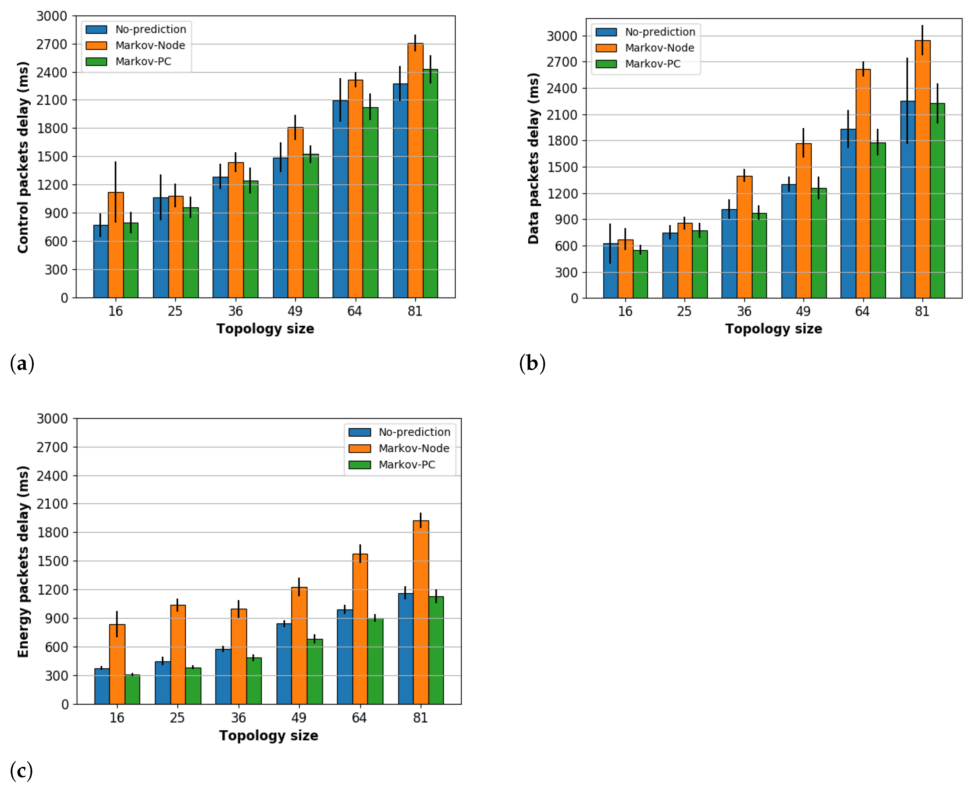
Figure 8a–c depicts the average delay for control, data, and energy packets, respectively. The first we observed is that the Markov-Node scheme obtained the highest delay in all the packet types, with a significant difference in the energy packet. In this case, the delay is from $65\%$ to $122\%$ higher than the delay in the No-Prediction scheme. Unlike the Markov-Node scheme, the Markov-PC scheme was able to maintain the control and data packets delay with respect to the No-Prediction scheme, but also it was able to reduce the delay up to $18\%$ in the case of the energy packets.

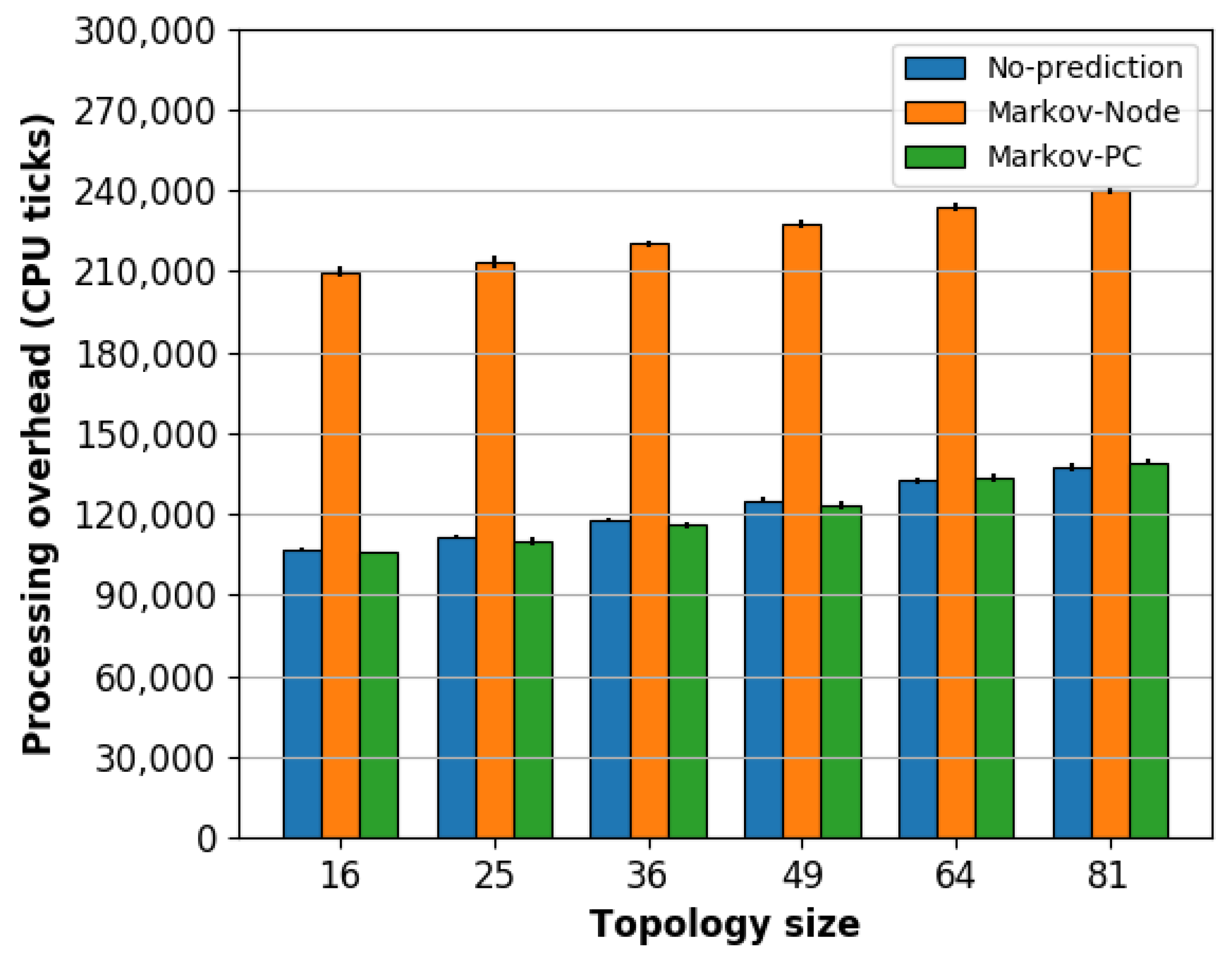
The increase in the delay using the Markov-Node scheme is caused by its processing overhead. As shown in Figure 9, the Markov-Node scheme doubles the processing overhead of the Markov-PC and No-Prediction schemes. This processing overhead delays energy packets forwarding. Furthermore, as energy and data updates have the same period, it also delays data packets forwarding. The Markov-PC and No-Prediction schemes have similar processing overheads. Thus, recalling the overhead and delivery rate results, despite the fact that the Markov-Node scheme reduces the number of energy packets in the network, the high delay caused by processing overhead could be affecting both energy packets and data packets delivery rate.

Summarizing, the Markov-PC scheme overcomes the Markov-Node scheme in all the metrics evaluated, except for the energy packets overhead. This means, executing the prediction in the SDN controller we obtain better accurate prediction and delivery rate, and less energy consumption, control packets overhead, delay and sensor nodes’ processing overhead. Then, with respect to the No-Prediction, the Markov-PC scheme reduces the energy consumption for topologies between 16 nodes and 49 nodes and increases it for topologies between 64 and 81 nodes. We also observed the Markov-PC scheme increases the energy packets delivery rate and reduces their delay. Moreover, in terms of control and data packets delivery rate and delay, the Markov-PC and No-Prediction scheme obtained a similar performance.

Thus, considering the whole picture, the Markov-PC scheme obtained better performance than the Markov-Node scheme, but also it provides benefits in terms of energy efficiency and network performance if compared with the No-Prediction scheme.

6. Conclusions

In this work, we proposed a centralized energy consumption prediction mechanism for WSN leveraged by SDN. Our hypothesis was that by moving the prediction processing overhead to the SDN controller we can improve the prediction accuracy and consequently the network performance. To test our hypothesis, we proposed an energy consumption model and implemented a prediction algorithm using Markov chain. Then, we evaluated the prediction and network performance when running the algorithm in every node and running it only in the SDN controller. Furthermore, to determine the real benefit, we compare the performance of both approaches with the case without prediction.

Results showed that by moving the prediction algorithm processing overhead from every node to the SDN controller we improved the prediction accuracy, delivery rate and delay of control, data and energy packets. Moreover, we reduced the control packets overhead, however there is a significant increase in the energy packets traffic.

Concerning the No-Prediction scheme, the Markov-PC scheme reduced the energy consumption, the control packets overhead and the energy packets delay. Furthermore, it improved the energy packets delivery rate. In the remaining metrics, excluding the energy packets overhead, the Markov-PC and the No-Predictions scheme obtained similar performance. These results show our centralized approach improves the prediction accuracy and network performance with less than $50\%$ of predictions attempts correct. Therefore, there is room to improve the prediction accuracy and, thus, the network performance.