Article

Modeling Pollutant Emissions: Influence of Two Heat and Power Plants on Urban Air Quality

by
Robert Cichowicz
* and
Maciej Dobrzański
Faculty of Architecture, Civil and Environmental Engineering, Lodz University of Technology, Al. Politechniki 6, 90-924 Lodz, Poland
*
Author to whom correspondence should be addressed.
Energies 2021, 14(17), 5218; https://doi.org/10.3390/en14175218
Submission received: 5 August 2021 / Revised: 11 August 2021 / Accepted: 17 August 2021 / Published: 24 August 2021

Abstract

:
Large industrial plants, power plants, and combined heat and power plants are popularly believed to be the main sources of point emissions, affecting both local and global air quality. This is because these installations emit significant amounts of pollutants at high altitudes every year. In this study, we investigate the impact of two solid fuel (hard coal)-fired CHP plants located within the urban agglomeration on the air quality of the city of Lodz in Poland (Europe). We used an OPA03 computer software to model the spatial distribution of pollutants. The results show that the annual average concentrations of pollutants were highest at an altitude of 25 m above ground level and decreased at lower measurement heights. The concentrations did not exceed permissible levels, reaching only 4% of national and international regulatory limits. We also made field measurements during the winter heating period, using an unmanned aerial vehicle (UAV) equipped with sensors to map the distributions of dust and gas pollutants in the areas with the highest concentrations of emissions from the two heat and power plants. Overall, the field measurements confirmed that it is not high-altitude emissions that have the greatest impact on local air quality.

1. Introduction

Air pollution is caused by the emission of gaseous, liquid, and solid substances in amounts that cause environmental damage, adversely affecting flora and fauna, water, soil, and human health [1]. The main air pollutants include nitrogen compounds (NO, NO2), carbon compounds (CO, CO2), sulfur dioxide (SO2), heavy metals (mercury, nickel, lead, arsenic, cadmium), hydrocarbons, and their derivatives, as well as particulate matter pollutants PM10, PM2.5, and PM1.0. Particulate matter pollutants have a negative impact on human health, both directly, by penetrating the body causing allergies and lung diseases, and indirectly, by acting as a carrier for heavy metals, microorganisms, and bacteria [2,3,4]. Therefore, it is important both to monitor the concentrations of pollutants in the air and to effectively control the amounts of pollutants emitted. Unfortunately, the regulations of the European Union set permissible dust concentrations only for the PM10 and PM2.5 fractions [5]. The permissible level of PM10 is 50 µg/m3 for the daily average and 40 µg/m3 for the annual average. For PM2.5, the maximum limit is 25 µg/m3 (annual average). According to WHO recommendations from 2005 [6], the average annual concentration of PM10 should not exceed 20 µg/m3, with a daily average of 50 µg/m3, whereas for PM2.5, the annual average concentration should not exceed 10 µg/m3 with a daily average of 25 µg/m3. No limits have been set for the PM1.0 fraction, although it is increasingly considered the most dangerous type of PM.
Particulate matter is not the only dangerous type of air pollution, however. Gaseous pollutants such as SO2, which is highly toxic with a suffocating odor, also pose a problem. Sulfur dioxide has a high specific gravity and relative density, which causes it to slowly spread through the atmosphere. It arises mainly as a result of burning solid and liquid fuels contaminated with sulfur (e.g., hard coal, crude oil) in combustion engines, power plants, and combined heat and power plants [7,8]. The amount of SO2 introduced into the environment largely depends on the quality of the fuel used. Sulfur compounds contribute to acidification of the environment, which leads to the formation of acid rain, lower soil fertility, inhibition of plant growth, and plant death [9]. Sulphur dioxide pollution is “seasonal”, in the sense that higher concentrations are observed during the winter/heating seasons, while in summer/vegetation seasons, there are lower concentrations of SO2. According to a European Union Directive 2008/50/EC [5], the permissible average daily concentration of SO2 is 125 µg/m3, and the permissible average hourly concentration is 350 µg/m3. These levels are the acceptable values for the protection of human health. The WHO [6] sets a much lower limit of 20 µg/m3 for the daily average. Unfortunately, the WHO guidelines do not provide a limit value for the annual average of SO2.
Nitrogen compounds NOx (NO, NO2) are another significant threat. These compounds are formed during the combustion of fuels at high temperatures, which leads to the oxidation of nitrogen contained in the fuels and in the atmosphere. The main sources of NO2 are road transport (so-called “linear emissions”) [10,11,12] and energy and heating systems (“point emissions”) [13]. The most dangerous nitrogen compounds are odorless and colorless nitrogen oxides and brown-colored suffocating NO2. Nitrogen oxides could contribute to photochemical smog and high ozone levels. However, more and more scientific works indicate to the contrary that nitrogen oxides can lead to ozone depletion in the air [14]. Nitrogen dioxide emissions are mainly caused by heavy traffic (linear emissions), as well as by heating systems and the energy sector (point emissions) [12]. The environmental damage caused by NOx includes eutrophication, which is associated with the degradation of terrestrial and aquatic ecosystems [15]. Nitrous oxides also contribute to the formation of tropospheric ozone [16] and acidification of the environment [17]. According to European standards, the daily average NO2 limit is 130 µg/m3 (these levels are the limit values for the protection of human health) [5]. According to WHO guidelines [6], the permissible average annual NO2 concentration is 40 µg/m3, and the hourly average is 200 µg/m3.
The basic method for determining the state of air quality is to measure pollutant concentrations. Stationary ground stations monitor pollutant concentrations in manual daily and automatic continuous systems [18,19,20]. However, the small number of such stations and the distance between them mean that the data they collect can only be used to evaluate the state of air quality on a global or national scale. It is not possible to assess the impact of individual emitters on the state of local air quality [21,22]. Local analyses are influenced by a number of important factors, such as wind direction and strength, meteorological conditions, topography, and roughness of the terrain [23,24,25]. To take into account all of these variables in the analysis, it would be necessary to have a complex network of numerous measuring stations located around the area. This is a very time-consuming and costly solution, so computer programs are used to simulate the concentrations and spread of pollutants based on detailed emitter data. Examples of such software include Aero 2010, Emitor, OPA03 [26], AERMOD [27], ENVI-met, and Austal 2000 [28].
Local analysis should also take into account the division of pollutant emissions into so-called “low” and “high” emissions. Low emissions are from pollution sources up to a height of about 40 m from ground level, i.e., from “line emitters” such as communication routes [29], “point emitters” such as the flue gas systems used in small industrial plants and individual households, and “surface emitters” such as densely built-up and inhabited residential quarters with individual heating systems [30]. “High emissions” are mainly produced by large industrial plants, power plants, and combined heat and power plants [31,32,33].
Here, we analyze an area of the city of Lodz (in the center of Poland, in Central Europe). The main sources of “high” and “point” emissions in Lodz are two coal-fired CHP plants. Despite technological progress and the introduction of substitutes in the form of biomass, hard coal is still the main raw material used to generate energy, with several hundred megagrams being burned each year. As a result, facilities such as combined heat and power plants are popularly considered to be the main emitters of air pollutants. In this study, we set out to determine whether the CHP plants are in fact the largest emitter of pollutants and the extent of their impact on the local environment.

2. Analyzed Objects

We analyzed emissions from the two main combined heat and power plants in the city of Lodz (Figure 1). Lodz is the third largest city in Poland (Central Europe) in terms of the number of inhabitants (area: 293.2 km2; population density: 2292.2 people/km2; population: 672,185). In the north-west part of the city, there is a combined heat and power plant designated with the number EC-3 (Figure 2A). This combustion installation includes five coal-fired steam boilers, including one capable of co-firing 20% biomass with hard coal, one steam boiler fired with light fuel oil, and three water boilers fired with heavy oil. The total thermal power is 804 MW, and the electric power is 205.85 MW. To the north and west of EC-3 there are industrial areas, and to the east and south there are single-family and multi-family residential areas. The gross development index in the area ranges from 0.5 to 1.0.
The second facility is the EC-4 CHP plant in the east of the city (Figure 2B). The EC-4 fuel combustion installation includes two coal-fired steam boilers, one biomass-fired steam boiler, one light fuel oil-fired steam boiler, and three coal-fired water boilers. The total thermal power of EC-4 is 820 MW, and its electric power output is 198 MW. In the immediate vicinity of EC-4 is an industrial and storage district. However, to the north and north-west nearby, there are single-family housing and collective housing areas. Towards the south, there are industrial areas, and towards the east and north-east, there are recreational and leisure areas with high greenery in the form of trees. The gross development index in this area ranges from 0.5 to 1.0. Significant sources of pollution in close proximity to both heat and power plants include busy roads leading to housing estates and out of the city. These line sources contribute to increasing the level of pollution in the area.

3. Methodology

The year 2019 was selected for analysis because it was the most recent before the COVID-19 pandemic, and so, there were no possible changes in pollutant emissions resulting from health restrictions. Detailed, real input data were provided for scientific purposes by Veolia Energia Łódź. OPA03 (Eko-Soft) [34] computer software was used to calculate the concentration of pollutants in the atmospheric air and their spatial dispersion. The program also includes the MAPS module, which is used for graphical interpretation of the results. The OPA03 system can analyze up to 900 point, surface, line, and equivalent emitters. The software enables calculation of boundary dust and gaseous emissions, with the diameter and height of the emitters as variables. The calculations were based on the legal regulation in force in Poland and the European Union [5,35], assuming “limit values” for selected substances in the air, “conditions” for which the reference values are determined (such as pressure and temperature), “periods” for which average reference values are provided, “conditions” for which reference values are considered acceptable, and reference values or “methods of modeling” levels of substances in the air. As part of the analysis, two dust pollutants PM10 and PM2.5 and two gaseous pollutants sulfur dioxide (SO2) and nitrogen dioxide (NO2) were selected. Due to the legal acts in force in Poland based on the regulations of the European Union [5,35], the background of pollutants for emitters higher than 100 m is not determined. In the analyzed cases, the background pollution was not taken into account, due to the fact that all chimneys/emitters are higher than 100 m (for the EC-3 CHP plant the height of the chimney is 120 m, and for the EC-4 CHP plant, the chimneys are 200 m and 250 m high). Pollution from the H120 stack was analyzed for the EC-3. However, for the EC-4 CHP plant, the basic configuration is the H250 chimney and the H200 chimney, to which five boilers are connected.
Data from the “wind rose” for the year 2019 (Figure 3) were entered into the program. In the city of Lodz in 2019, the prevailing winds were from the west (13%), north-west (14%), and south-west (11%), while northerly and southerly winds (about 4%) were much less frequent, and easterly winds were the least frequent (2%). The year 2019 can be considered typical in terms of these meteorological parameters.
To obtain more accurate calculation data, 2019 was divided into three sub-periods: the “summer” period (from April 1 to September 30) and two “winter/heating” periods. In the “1st winter/heating period” (from 1 January to 31 March), the average air temperatures were lower (Table 1) than those in the “2nd winter/heating period” (from 1 October to 31 December). This is a typical phenomenon in the region of Central Europe. As a result, there is greater demand for thermal energy in the period from January to March, which translates into higher pollutant emissions.
Three heights of pollution dispersion were selected for analysis: 1.5, 14, and 25 m. The height of 1.5 m is the minimum measurement height recommended in national regulations based on European Union directives [5,17,35]. The height of 14 m is the height at which anemometers (devices used to measure the speed of movement of gases and liquids) are located. The height of 25 m is the average height of skyscrapers in Lodz.
Field measurements were also made, using an unmanned aerial vehicle (UAV) equipped with mobile measuring equipment [37,38]. The measuring equipment included a laser-scattered (LS) sensor to measure PM10, PM2.5, and PM1.0 (10,000 particles per second) and electrochemical (EC)-type sensors to measure H2S (3 ppb–1 ppm), O2 (0.20–100%), and SO2 (0.5–2000 ppm). Measurements were made at the heights of 1.5, 14, 25, 30, and 50 m, in those places where the numerical analysis had predicted the highest concentrations of emissions from the two power stations. The field measurements were compared to the results of the numerical analysis.

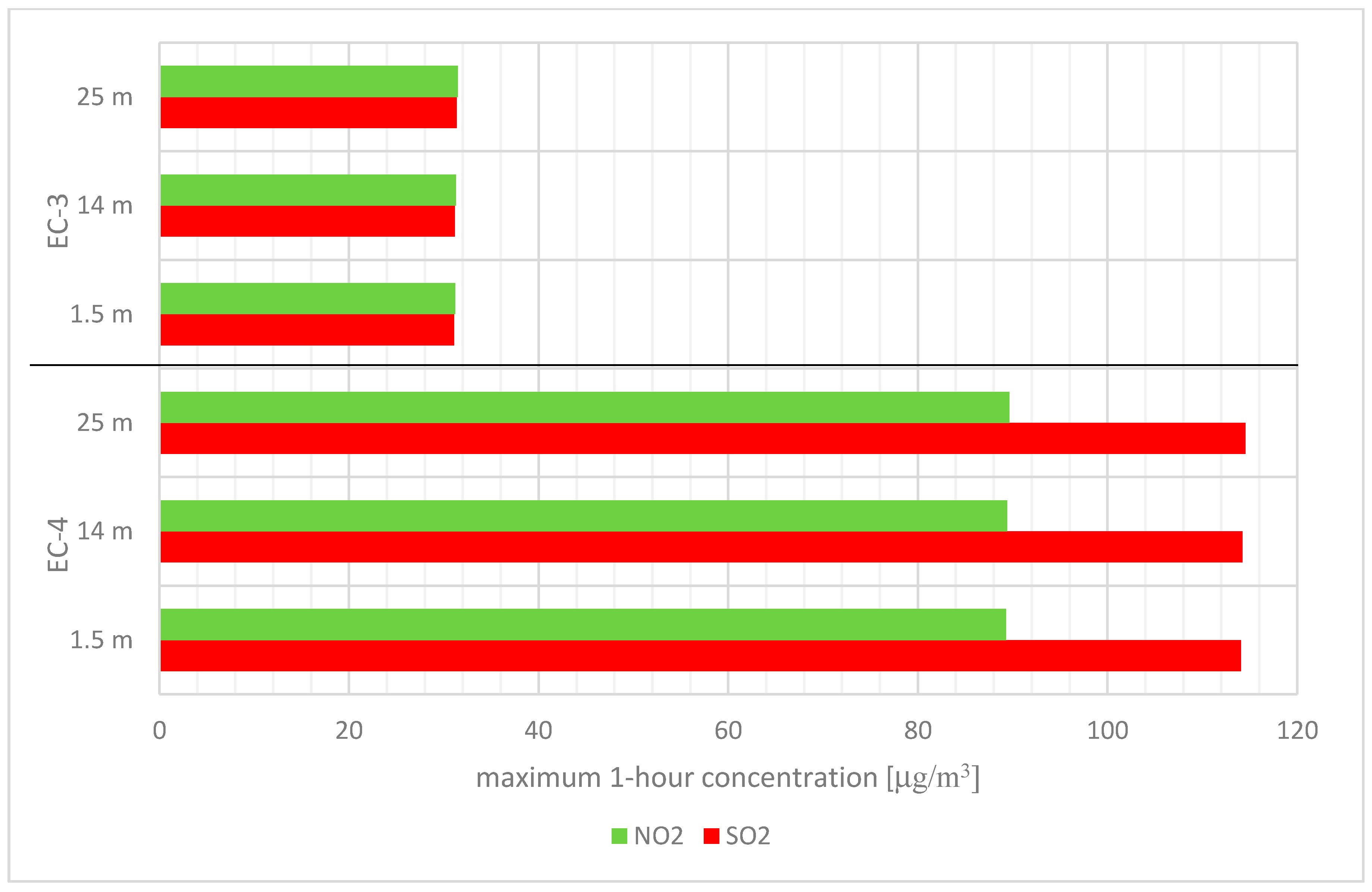
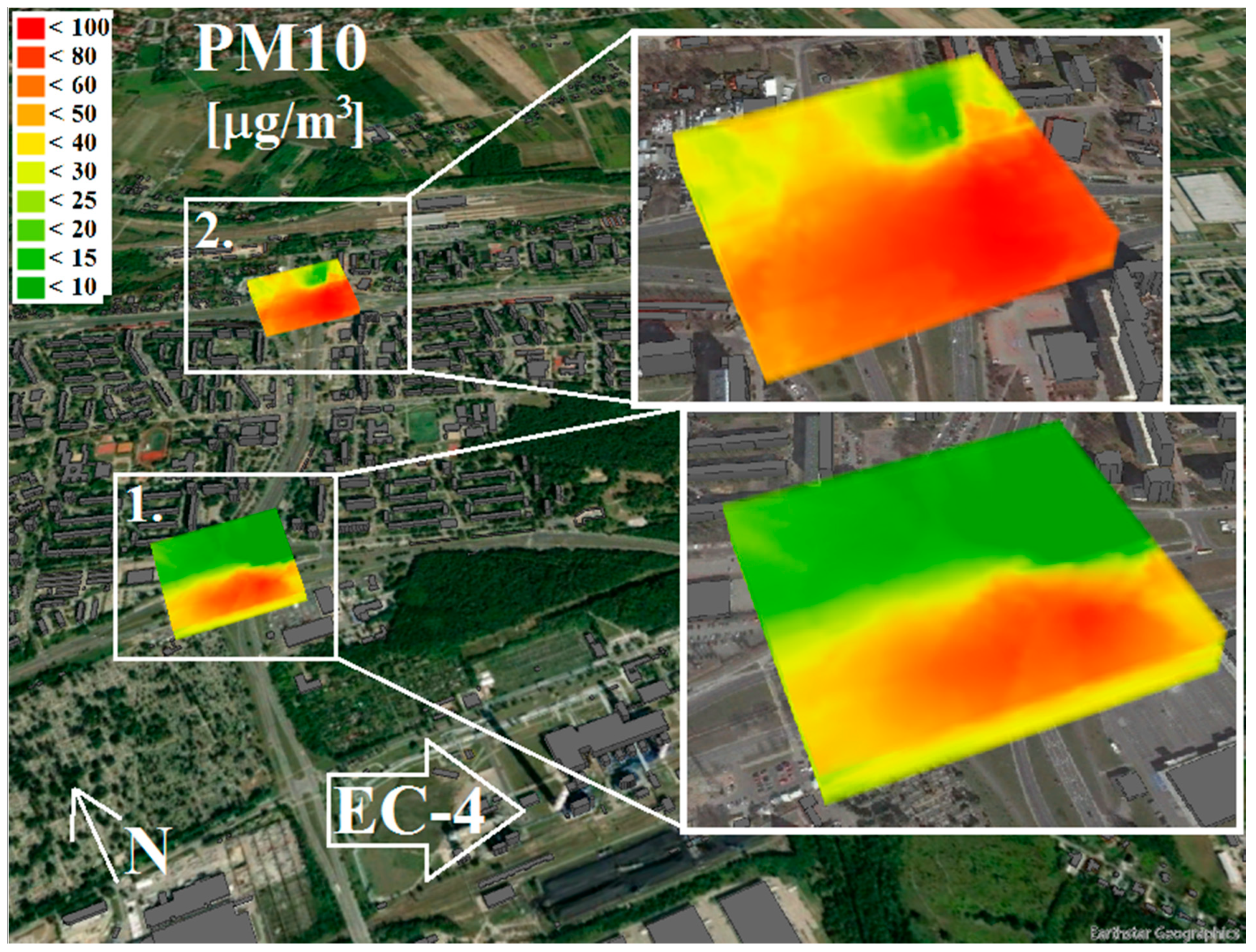
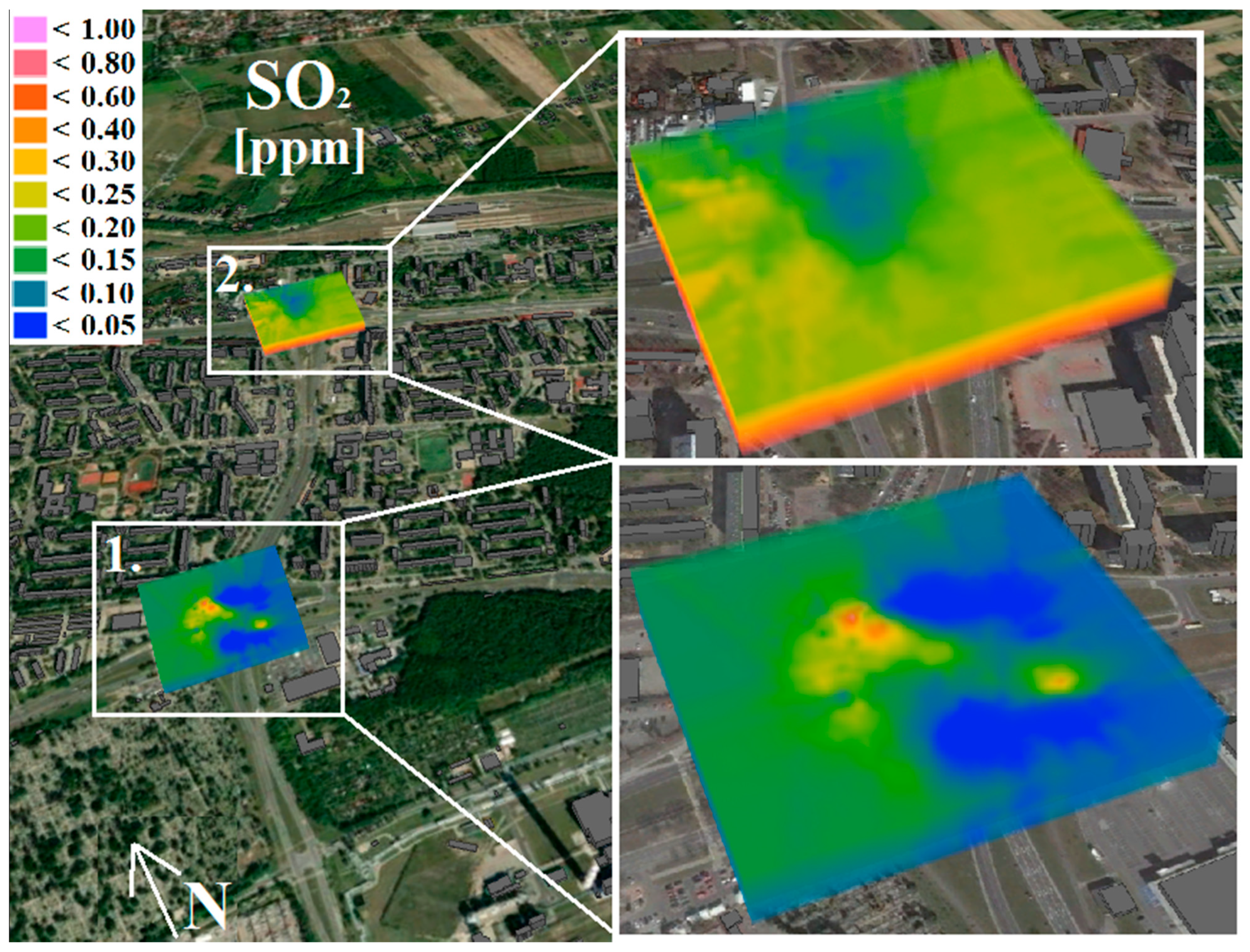
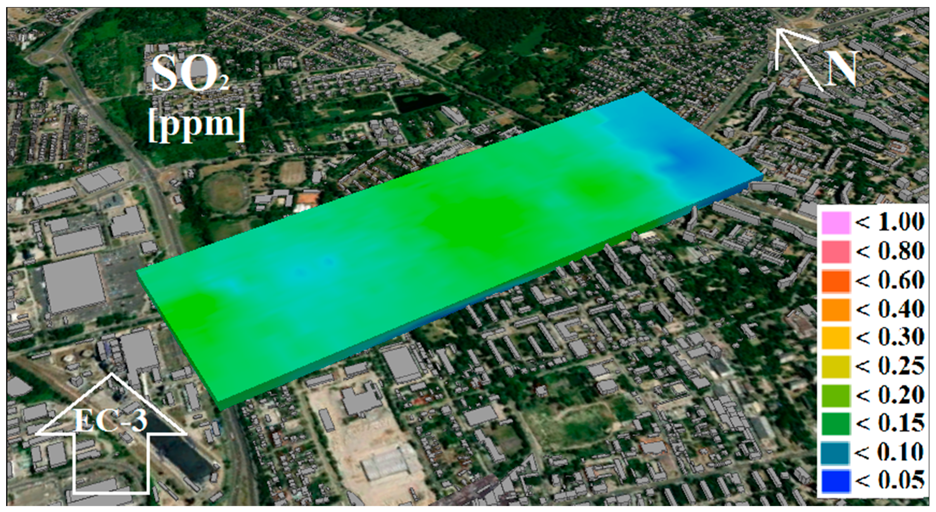
4. Results and Discussion

The total emissions of pollutants in 2019 were calculated based on measurement data provided by the network heat supplier, Veolia Energia Łódź (Table 2). Despite the comparable power of the two heat and power plants, “EC-4” emitted higher total emissions of pollutants than “EC-3”. This was probably caused by the higher fuel consumption of the EC-4 CHP plant, due to the greater demand for power in this area of the city of Lodz.
Based on the data in Table 2 and the operating time of individual boilers, the maximum hourly emissions of pollutants (Table 3) from the EC-3 and EC-4 CHP plants in 2019 and the average hourly emissions (Table 4) for selected sub-periods were also calculated. The highest average hourly emissions (kg/h) and maximum hourly emissions occurred in the “1st winter and heating period”. Most likely, this was associated with the low atmospheric temperatures (Table 1) and the need to generate more thermal power for residential properties. In the coldest periods, all CHP boilers work to cover the demand for heating. The atmospheric temperatures in the “2nd winter/heating period” were on average 3.9 °C higher, and there was, therefore, a lower demand for thermal energy.
The lowest average hourly emissions (kg/h) occurred in the “summer period”, when, due to the higher atmospheric temperatures, the combined heat and power plants needed to generate only enough energy to provide domestic hot water to premises connected to the heating network and to cover demand for electricity and, therefore, burned less fuel. On the other hand, the highest average hourly emissions (kg/h) occurred in the “I winter-heating period“, when, due to the lower atmospheric temperatures (Table 1), the combined heat and power plants needed to generate the greatest amount of energy. The permissible emissions of pollutants were not exceeded in any of the sub-periods, thanks to the high quality standards for exhaust gasses maintained by environmental protection devices, such as electrostatic precipitators and flue gas desulphurization installations.
In the next stage of the analysis, we simulated the environmental impact of the CHP plants. The value of the load of imitated pollutants was converted into the concentration of the pollutants in the air. The average annual and maximum hourly concentrations were taken into account for three heights: 1.5 m, 14 m, and 25 m. We also analyzed the spatial dispersion of the selected pollutants in the vicinity of the two CHP plants.
As can be seen from Figure 4 and Figure 5, the EC-4 CHP plant was associated with the highest calculated average annual concentrations of pollutants in the air. This is consistent with the higher emission (kg) of pollutants from EC-4 compared to EC-3. Calculations made using OPA03 software for the EC-4 CHP plant show that the highest calculated annual average concentrations for PM10 was still very low, amounting to only about 0.04% of the reference value of 40 µg/m3 stipulated in Directive 2008/50/EC [5]. Similar conclusions apply to the annual average concentrations of PM2.5, which were also about 0.03% of the reference value of 25 µg/m3. Much higher concentrations were calculated for gaseous pollutants than for dust pollutants. The average annual concentration of SO2 was 4.24% of the reference value of 20 µg/m3 [6]. The highest average annual concentration of nitrogen compounds, including both NO2 and NO converted to NO2, amounted to 1.73% of the reference value (40 µg/m3). Detailed calculations made using OPA03 software for EC-3 show that the highest of the annual concentrations for PM10 and PM2.5 were only 0.02 and 0.01% of the permissible values, respectively. As in the case of EC-4, lower concentrations than the permissible values were recorded for gaseous pollutants in EC-3. The average annual concentration of SO2 reached 2.46% of the limit value and, for NO2, amounted to 1.17% of the limit value. Generally, the concentrations of pollutants increased at higher altitudes (1.5 m, 14 m, and 25 m). The highest concentrations were recorded primarily at the height of 25 m.
Overall, the average annual concentrations of the analyzed pollutants amounted to a maximum of 4% of the relevant permissible values. This is probably due to the flue gas cleaning systems used in both CHP plants, which reduce the emission of pollutants into the atmosphere. Another important parameter in the analysis of the impact of the CHP plant on air quality is the maximum 1 h concentration (Figure 6). In general, the changes in the concentrations of gaseous pollutants that occurred at increasing heights were negligible. In the case of the EC-4 plant, the maximum 1 h concentration of SO2 was approximately 114.5 µg/m3, which is approximately 33% of the reference value of 350 µg/m3. For NO2, the concentration was about 89.5 µg/m3, i.e., about 45% of the reference value of 200 µg/m3. In the case of the EC-3 plant, the values for SO2 were around 31 µg/m3, which is about 9% of the reference value (350 µg/m3). For NO2, the hourly concentration was about 31.5 µg/m3, which is about 16% of the reference value (200 µg/m3).
To analyze more fully the impact of the heat and power plant on the surroundings, we made dispersion maps. The black points on the maps show the location of the EC-3 and EC-4 CHP plants and the administrative borders of the city of Lodz. Figure 7 shows the dispersions of SO2 from the EC-4 plant at heights of 1.5 m, 14 m, and 25 m.
The values range from 0.2 µg/m3 to 0.8 µg/m3, which is between 1% and 4% of the reference value. The area with SO2 concentrations of 0.8 µg/m3 doubled as the measurement height increased from 1.5 m to 25 m (Figure 7). The SO2 pollution from EC-4 spread in accordance with the wind rose shown in Figure 3. The pollution spread mainly towards the north, north-east, and east, i.e., following the prevalent winds for Lodz in 2019. Concentrations of SO2 above 0.2 µg/m3 covered about 35% of the area of the city of Lodz.
Figure 8 shows the dispersions of SO2 pollutants from EC-3 at heights of 1.5, 14, and 25 m. The average annual concentrations range from 0.2 to 0.5 µg/m3. The area with a concentration of SO2 equal to or greater than 0.5 µg/m3 doubled as the measurement height increased from 1.5 m to 14 m. However, at a height of 25 m, it tripled relative to the concentration at 1.5 m. The dispersion of pollutants again coincided with the established wind rose. The impact of pollutants from EC-3 was negligible, amounting to a maximum of 3.4% of the reference value. Hao et al. report similar results [33]. Concentrations of SO2 from EC-3 above 0.2 µg/m3 (Figure 8) covered about 13% of the area of the city of Lodz.
Figure 9 shows an example of the dispersion of NO2 pollutants from the EC-4 heat and power plant at heights of 1.5, 14, and 25 m. As can be seen, the highest annual average NO2 concentration is 0.6 µg/m3. The area with a concentration of 0.6 µg/m, which constitutes 1.5% of the reference value, is 40 µg/m3. Ghermandi et al. also showed that the limit values were not exceeded during their computer analysis of NO2 emissions from a CHP plant in San Marino [39]. The dispersion of NO2 pollutants also coincided with the wind rose for Lodz for 2019.
Figure 10 shows the spatial dispersion of PM10 from EC-4. The distribution of pollutants at 1.5 m is shown on the left, and the distribution at 25 m is shown on the right. The concentrations of pollutants are in the range of 0.003–0.015 µg/m3, which is 0.007–0.03% of the reference value. The highest values of 0.015 µg/m3 occurred only at a height of 25 m. Of all the pollutants, PM10 had the largest area of influence.
Summarizing the results of analysis using the OPA03-Maps program, the average annual concentrations range from thousandths of a percent to several percent of the permissible values. This can be attributed to the use of dedusting devices, flue gas denitrification, and desulphurization installations, as well as various types of filters with high dedusting efficiency. Both CHP plants, thus, have a negligible impact on air quality. The highest concentrations of pollutants occurred at a height of 25 m. Due to the movement of air masses, the concentrations of pollutants from the heat and power plants fall significantly as the measuring height reduces. This is very important because, as shown by the pollution dispersion maps, the main areas to which the pollutants are transported by the predominant wind directions are mainly collective and individual residence areas, as well as green areas used by residents for relaxation and recreation.
Field measurements were made with the use of UAV to verify the impact of the CHP plants on air quality. The field measurements were taken during the heating season in the areas with the highest concentrations of pollutants from the heat and power plants, according to the analysis in OPA03. In the case of EC-4, these were two intersections of the main streets in the city, indicated in Figure 11.
As shown in Figure 11, in location no. 1, located closer to EC-4, the concentration of PM10 varied in the range 27.57–84.76 µg/m3. In location no. 2, the concentration of PM10 varied in the range 44.05–80.37 µg/m3. According to the analysis in OPA03, the highest average annual concentration of PM10 particulate pollutants emitted from EC-4 was 0.016 µg/m3. The concentrations recorded in the field measurements were 5000 times higher. This proves the negligible impact of the EC-4 heat and power plant on air quality. It can be assumed that the high measured concentrations of PM10 were caused by “low emissions” from transport and individual heating systems, which in Poland, do not have to meet high standards for exhaust gas treatment, such as those set for municipal heat and power plants. The concentration of SO2 measured for location no. 1 varied in the range 0.06–0.40 ppm (Figure 12), i.e., about 170–1130 µg/m3. In location no. 2, the concentration of SO2 varied in the range 0.15–0.40 ppm (420–1130 µg/m3). According to the analysis in OPA03, the maximum hourly concentration SO2 emitted from EC-4 was 115 µg/m3. This means that the SO2 concentrations measured in location no. 2 were almost 10 times higher than the emissions from the combined heat and power plant. As in the case of particulate pollutants, this can be explained by “low emissions” providing the dominant share of the total concentration of sulfur dioxide.
Another area we analyzed was at a distance of approx. 1.5 km from the EC-3 heat and power plant (Figure 13 and Figure 14). The concentration of PM10 varied spatially in a narrow range, from 13.52 to 38.25 µg/m3 (Figure 13). The real concentrations were, thus, more than 5000 times higher than the emissions from EC-3 determined on the basis of OPA03 modeling (the highest annual average concentration was 0.007 µg/m3).
On the other hand, field measurements of the SO2 concentration (Figure 14) showed variations in the range 0.01–0.14 ppm (about 30–390 µg/m3). The real concentrations were more than 12 times higher than the maximum hourly value of about 32 µg/m3 calculated in OPA03. As in the case of EC-4, the EC-3 CHP plant was, therefore, found to emit only a small proportion of the actual concentration of pollutants. This proves that the main sources of the analyzed pollutants were not the CHP plants, but probably “low” and “linear” emissions from transport and individual heating.

5. Conclusions

Based on our analysis of the dispersion of atmospheric air pollutants in 2019, the concentrations of pollutants from the EC-3 and EC-4 municipal heat and power plants do not exceed the permissible values and do not independently present a threat to human health. Organizational units of Veolia Energia Łódź, which manage facilities including the EC-3 and EC-4 CHP plants, comply with the applicable regulations and implement plans to limit emissions into the air, using desulphurization installations and flue gas cleaning devices. However, field measurements showed that total emissions including other sources, i.e., “linear emissions” in the form of transportation and “low emissions” from home furnaces, do pose a real threat to environmental health and safety, because the concentrations of pollutants exceed permissible levels in the air. In order to improve air quality, it is necessary to act to reduce the amount of pollution emitted from all sources. In particular, it is possible to mention a reduction in the number of vehicles used for public transport or replacing them with electric vehicles and the replacement of individual coal-fired boilers with gas or electric heat sources.
Our numerical analysis in OPA03 software showed that at lower measuring heights, the concentrations of pollutants from EC-3 and EC-4 decreased, and the area with the highest average annual concentrations approximately doubled. However, the field measurements showed that the highest concentrations of the pollutants were recorded close to the ground surface and decreased at higher altitudes. This demonstrates the direct impact of “low emissions” on air quality. Pollutants emitted, for example, from vehicles and individual heating systems, accumulate at the ground surface and, then, through air movement, are lifted to higher parts of the atmosphere. There, there is a gradual dilution/reduction in their concentration by mixing with air. Dispersion maps generated based on the analysis in OPA03 and field measurements confirmed that the spread of pollutants was mostly influenced by wind speed and direction. Another very important factor influencing the condition of atmospheric air is the season. As shown in Table 4, higher emissions of pollutants occur during the winter-heating period. In the “winter/heating period”, in addition to sources of air pollution that are active throughout the year, it is necessary to take into account those that are used seasonally, e.g., individual heating systems. In colder weather, there is more demand for heat energy, and therefore, higher levels of pollutants are produced both by CHP plants (“high emissions”) and home furnaces (“low emissions”).
The combined use of field measurements and computer simulations constitutes a new approach to analyzing air quality, making it possible to select areas for field analysis and to verify the impact of emitters on air quality. This method can be implemented anywhere in the world, in relation to various emitters of air pollutants.

Author Contributions

Conceptualization, R.C. and M.D.; methodology, R.C. and M.D.; software, M.D. and R.C.; writing—original draft, R.C. and M.D., review and editing, R.C. All authors have read and agreed to the published version of the manuscript.

Funding

This study was conducted as part of the research project entitled “Spatial analysis of air pollution changes in the Lodz agglomeration (in Polish: Analiza przestrzenna zmian stanu zanieczyszczenia powietrza w aglomeracji łódzkiej)”, which was co-financed by approx. 80% by the Provincial Fund for Environmental Protection and Water Management in Lodz (in Polish: Wojewódzki Fundusz Ochrony Środowiska i Gospodarki Wodnej w Łodzi). 590/BN/D/2018.

Institutional Review Board Statement

Not applicable.

Informed Consent Statement

Not applicable.

Data Availability Statement

Data available on request.

Conflicts of Interest

The authors declare no conflict of interest.

References

  1. Yang, G.; Wang, Y.; Zeng, Y.; Gao, G.F.; Liang, X.; Zhou, M.; Wan, X.; Yu, S.; Jiang, Y.; Naghavi, M.; et al. Rapid health transition in China, 1990–2010: Findings from the global burden of disease study 2010. Lancet 2013, 381, 1987–2015. [Google Scholar] [CrossRef]
  2. Sówka, I.; Kobus, D.; Skotak, K.; Zathey, M.; Merenda, B.; Paciorek, M. Assessment of the health risk related to air pollution in selected polish health resorts. J. Ecol. Eng. 2019, 20, 132–145. [Google Scholar] [CrossRef]
  3. Pope, C.A. Mortality effects of longer term exposures to fine particulate air pollution: Review of recent epidemiological evidence. Inhal. Toxicol. 2007, 19, 33–38. [Google Scholar] [CrossRef] [PubMed]
  4. Almeida, S.M.; Pio, C.; Freitas, M.; Reis, M.; Trancoso, M. Source apportionment of fine and coarse particulate matter in a sub-urban area at the Western European Coast. Atmospheric. Environ. 2005, 39, 3127–3138. [Google Scholar] [CrossRef]
  5. UNION, PEAN. Directive 2008/50/EC of the European Parliament and of the Council of 21 May 2008 on ambient air quality and cleaner air for Europe. Off. J. Eur. Union 2008, 29, 169–212. Available online: http://data.europa.eu/eli/dir/2008/50/oj (accessed on 12 June 2021).
  6. World Health Organization. Who Air Quality Guidelines for Particulate Matter, Ozone, Nitrogen Dioxide and Sulfur Dioxide. Global Update 2005. Summary of Risk Assessment, 2005. Available online: https://www.euro.who.int/en/health-topics/environment-and-health/air-quality/publications/pre2009/air-quality-guidelines.-global-update-2005.-particulate-matter,-ozone,-nitrogen-dioxide-and-sulfur-dioxide (accessed on 12 June 2021).
  7. Meng, M.; Zhou, J. Has air pollution emission level in the Beijing–Tianjin–Hebei region peaked? A panel data analysis. Ecol. Indic. 2020, 119, 106875. [Google Scholar] [CrossRef]
  8. World Health Organization. Review of Evidence on Health Aspects of Air Pollution—REVIHAAP Project. World Health Organization 309. 2013. Available online: http://www.euro.who.int/en/health-topics/environment-and-health/air-quality/publications/2013/review-of-evidence-on-health-aspects-of-air-pollution-revihaap-project-finaltechnical-report (accessed on 2 July 2021).
  9. Larssen, S.; Hagen, O.L. Air Quality in Europe, 1993. A Pilot Report. November 1996. European Environment Agency. Available online: https://www.eea.europa.eu/publications/2-9167-057-X (accessed on 12 June 2021).
  10. Kousoulidou, M.; Ntziachristos, L.; Mellios, G.; Samaras, Z. Road-transport emission projections to 2020 in European urban environments. Atmospheric. Environ. 2008, 42, 7465–7475. [Google Scholar] [CrossRef]
  11. Kota, S.; Zhang, H.; Chen, G.; Schade, G.; Ying, Q. Evaluation of on-road vehicle CO and NOx national emission inventories using an urban-scale source-oriented air quality model. Atmospheric. Environ. 2014, 85, 99–108. [Google Scholar] [CrossRef]
  12. Mohsen, M.; Ahmed, M.B.; Zhou, J.L. Particulate matter concentrations and heavy metal contamination levels in the railway transport system of Sydney, Australia. Transp. Res. Part D Transp. Environ. 2018, 62, 112–124. [Google Scholar] [CrossRef]
  13. Cichowicz, R.; Wielgosiński, G.; Fetter, W. Effect of wind speed on the level of particulate matter PM10 concentration in atmospheric air during winter season in vicinity of large combustion plant. J. Atmospheric. Chem. 2020, 77, 35–48. [Google Scholar] [CrossRef]
  14. Cocks, A.T.; Kallend, A.S.; Marsh, A.R.W. Dispersion limitations of oxidation in power plant plumes during long-range transport. Nat. Cell Biol. 1983, 305, 122–123. [Google Scholar] [CrossRef]
  15. Bednova, O.V.; Kuznetsov, V.A.; Tarasova, N.P. Eutrophication of an urban forest ecosystem: Causes and effects. Dokl. Earth Sci. 2018, 478, 124–128. [Google Scholar] [CrossRef]
  16. Diamond, M.S.; Wood, R. Limited Regional aerosol and cloud microphysical changes despite unprecedented decline in nitrogen oxide pollution during the February 2020 COVID-19 shutdown in China. Geophys. Res. Lett. 2020, 47, 2020 088913. [Google Scholar] [CrossRef]
  17. Obolkin, V.; Khodzher, T.; Sorokovikova, L.; Tomberg, I.; Netsvetaeva, O.; Golobokova, L. Effect of long-range transport of sulphur and nitrogen oxides from large coal power plants on acidification of river waters in the Baikal region, East Siberia. Int. J. Environ. Stud. 2016, 73, 452–461. [Google Scholar] [CrossRef]
  18. Nagl, C.; Spangl, W.; Buxbaum, I. Sampling Points for Air Quality. Representativeness and Comparability of Measurement in Accordance with Directive 2008/50/EC on Ambient Air Quality and Cleaner Air for Europe. Policy Department for Economic, Scientific and Quality of Life Policies, Directorate-General for Internal Policies. PE 631.055-March 2019. Available online: http://www.europarl.europa.eu/RegData/etudes/STUD/2019/631055/IPOL_STU(2019)631055_EN.pdf (accessed on 12 June 2021).
  19. Chen, W.; Wang, F.; Xiao, G.; Wu, K.; Zhang, S. Air quality of beijing and impacts of the new ambient air quality standard. Atmosphere 2015, 6, 1243–1258. [Google Scholar] [CrossRef] [Green Version]
  20. Kuklinska, K.; Wolska, L.; Namiesnik, J. Air quality policy in the U.S. and the EU–A review. Atmospheric. Pollut. Res. 2015, 6, 129–137. [Google Scholar] [CrossRef]
  21. Atamaleki, A.; Zarandi, S.M.; Fakhri, Y.; Mehrizi, E.A.; Hesam, G.; Faramarzi, M.; Darbandi, M. Estimation of air pollutants emission (PM10, CO, SO2 and NOx) during development of the industry using AUSTAL 2000 model: A new method for sustainable development. MethodsX 2019, 6, 1581–1590. [Google Scholar] [CrossRef]
  22. Cichowicz, R.; Dobrzański, M. 3D spatial analysis of particulate matter (PM10, PM2.5 and PM1.0) and gaseous pollutants (H2S, SO2 and VOC) in urban areas surrounding a large heat and power plant. Energies 2021, 14, 4070. [Google Scholar] [CrossRef]
  23. Keshavarzian, E.; Jin, R.; Dong, K.; Kwok, K.C. Effect of building cross-section shape on air pollutant dispersion around buildings. Build. Environ. 2021, 197, 107861. [Google Scholar] [CrossRef]
  24. Ramponi, R.; Blocken, B.; De Coo, L.B.; Janssen, W.D. CFD simulation of outdoor ventilation of generic urban configurations with different urban densities and equal and unequal street widths. Build. Environ. 2015, 92, 152–166. [Google Scholar] [CrossRef] [Green Version]
  25. Yuan, C.; Ng, E.Y.Y. Building porosity for better urban ventilation in high-density cities–A computational parametric study. Build. Environ. 2012, 50, 176–189. [Google Scholar] [CrossRef]
  26. Łatuszyńska, M.; Strulak-Wójcikiewicz, R. A model for assessing the environmental impact of transport. Oper. Res. Decis. 2013, 23, 67–80. [Google Scholar] [CrossRef]
  27. Abu-Allaban, M.; Abu-Qdais, H. Impact assessment of ambient air quality by cement industry: A case study in jordan. Aerosol Air Qual. Res. 2011, 11, 802–810. [Google Scholar] [CrossRef]
  28. Paas, B.; Schneider, C. A comparison of model performance between ENVI-met and Austal2000 for particulate matter. Atmospheric. Environ. 2016, 145, 392–404. [Google Scholar] [CrossRef]
  29. Ropkins, K.; Beebe, J.; Li, H.; Daham, B.; Tate, J.; Bell, M.; Andrews, G. Real-world vehicle exhaust emissions monitoring: Review and critical discussion. Crit. Rev. Environ. Sci. Technol. 2009, 39, 79–152. [Google Scholar] [CrossRef]
  30. Gebremedhin, A. Introducing district heating in a norwegian town–potential for reduced local and global emissions. Appl. Energy 2012, 95, 300–304. [Google Scholar] [CrossRef]
  31. Cichowicz, R.; Dobrzański, M. Spatial analysis (measurements at heights of 10 m and 20 m above ground level) of the concentrations of particulate matter (PM 10, PM 2.5, and PM 1.0) and gaseous pollutants (H2S) on the university campus: A case study. Atmosphere 2021, 12, 62. [Google Scholar] [CrossRef]
  32. Lee, H.; Yoo, J.; Kang, M.; Kang, J.; Jung, J.; Oh, K. Evaluation of concentrations and source contribution of PM 10 and SO2 emitted from industrial complexes in Ulsan, Korea: Interfacing of the WRF–CALPUFF modeling tools. Atmospheric. Pollut. Res. 2014, 5, 664–676. [Google Scholar] [CrossRef] [Green Version]
  33. Hao, J.; Wang, L.; Shen, M.; Li, L.; Hu, J. Air quality impacts of power plant emissions in Beijing. Environ. Pollut. 2007, 147, 401–408. [Google Scholar] [CrossRef]
  34. Calculation Software for Pollutant Concentration Analysis. Eko-Soft company from Poland. Available online: http://www.eko-soft.com.pl/sysopa.htm (accessed on 12 June 2021).
  35. Polish Legal Act. Rozporządzenie Ministra Środowiska z Dnia 26 Stycznia 2010 r. w Sprawie Wartości Odniesienia Dla Niektórych Substancji W Powietrzu. Available online: http://isap.sejm.gov.pl/isap.nsf/DocDetails.xsp?id=wdu20100160087 (accessed on 12 June 2021).
  36. Meteorological Data. Available online: https://danepubliczne.imgw.pl/data/dane_pomiarowo_obserwacyjne/dane_meteorologiczne/miesieczne/synop/2019/ (accessed on 12 June 2021).
  37. Jumaah, H.; Kalantar, B.; Halin, A.; Mansor, S.; Ueda, N.; Jumaah, S. Development of UAV-based PM2.5 monitoring system. Drones 2021, 5, 60. [Google Scholar] [CrossRef]
  38. Caillouet, C.; Giroire, F.; Razafindralambo, T. Optimization of mobile sensor coverage with UAVs. In Proceedings of the IEEE INFOCOM 2018-IEEE Conference on Computer Communications, Honolulu, HI, USA, 15–19 April 2018; pp. 622–627. [Google Scholar]
  39. Ghermandi, G.; Fabbi, S.; Arvani, B.; Veratti, G.; Bigi, A.; Teggi, S. Impact assessment of pollutant emissions in the atmosphere from a power plant over a complex terrain and under unsteady winds. Sustainability 2017, 9, 2076. [Google Scholar] [CrossRef] [Green Version]
Figure 1. Location of the EC-3 and EC-4 CHP plants in the city of Lodz in Poland, Europe (photo background source: Google Earth Pro).
Energies 14 05218 g001
Figure 2. Location and immediate surroundings of the heat and power plant EC-3 (A) and EC-4 (B) (photo background source: Google Earth Pro).
Energies 14 05218 g002
Figure 3. Wind rose for the city of Lodz in 2019 (own study based on data from source: [36]).
Energies 14 05218 g003
Figure 4. The highest annual average concentration of particulate matter pollutants at the height of 1.5, 14, and 25 m for the EC-3 and EC-4 CHP plants based on the results from OPA03.
Energies 14 05218 g004
Figure 5. The highest annual average concentration of gaseous pollutants at the height of 1.5, 14, and 25 m for the EC-3 and EC-4 CHP plants based on the results from OPA03.
Energies 14 05218 g005
Figure 6. The highest hourly concentration of gaseous pollutants at the height of 1.5 m, 14 m, and 25 m for the EC-3 and EC-4 CHP plants based on the results from OPA03.
Energies 14 05218 g006
Figure 7. Distribution of annual average SO2 concentrations of 1.5 m, 14 m, and 25 m surrounded by EC-4 in 2019 based on the results from OPA03.
Energies 14 05218 g007
Figure 8. Distribution of annual average SO2 concentrations at the height of 1.5, 14, and 25 m surrounded by EC-3 in 2019 based on the results from OPA03.
Energies 14 05218 g008
Figure 9. Distribution of annual average NO2 concentrations at the height of 1.5 m, 14 m, and 25 m surrounded by EC-4 in 2019 based on the results from OPA03.
Energies 14 05218 g009
Figure 10. Distribution of annual average concentrations of PM10 at the height of 1.5 m and 25 m surrounded by EC-4 in 2019 based on the results from OPA03.
Energies 14 05218 g010
Figure 11. Spatial distribution of PM10 concentration for a selected location in the vicinity of EC-4.
Energies 14 05218 g011
Figure 12. Spatial distribution of SO2 concentration for a selected location in the vicinity of EC-4.
Energies 14 05218 g012
Figure 13. Spatial distribution of PM10 concentration for a selected location in the vicinity of EC-3.
Energies 14 05218 g013
Figure 14. Spatial distribution of SO2 concentration for a selected location in the vicinity of EC-3.
Energies 14 05218 g014
Table 1. Average monthly temperatures in 2019 for Lodz (own study based on data from source: [36]).
MonthJanuaryFebruaryMarchAprilMayJune
Temperature [°C]−1.72.65.710.112.422.2
MonthJulyAugustSeptemberOctoberNovemberDecember
Temperature [°C]18.720.214.010.46.23.2
Table 2. Emission of pollutants from EC-3 and EC-4 in 2019 (own calculations based on data from Veolia Energia Łódź).
EC-3 CHP Plant
Emitor:Emission [kg]
PM10PM2.5SO2NO2
H120-K1, K2,
K3, K6, K9
11,080.374748.73578,788.3583,515.8
EC-4 CHP Plant
H250-K710,645.884562.52228,952.5300,471.9
H200-K24783.522050.08135,430.6151,654.8
H200-K33286.641408.5672,609.9171,419.2
H200-K4, K51267.21543.0946,013.729,063.1
H200-K6808.78346.6226,176.014,290.0
Table 3. Maximum hourly emissions of pollutants for EC-3 and EC-4 CHP plants in 2019 (own calculations based on data from Veolia Energia Łódź).
EC-3 CHP Plant
EmitorMaximum Hourly Emission [kg/h]
H120PM10PM2.5SO2NO2
2.6671.143128.81144.20
EC-4 CHP Plant
PM10PM2.5SO2NO2
H250-K74.7602.040103.4079.30
H200-K23.4301.470189.9048.96
H200-K30.8960.38424.1234.49
H200-K4, K56.2862.694122.8386.70
H200-K68.0853.465285.95145.7
Table 4. Average hourly emissions of pollutants for the EC-3 and EC-4 CHP plants, divided into sub-periods (own calculations based on data from Veolia Energia Łódź).
EC-3 CHP Plant
Emitor:Period:Average Hour Emission [kg/h]
PM10PM2.5SO2NO2
H120-K1, K2,
K3, K6, K9
Summer period0.910.3934.6534.80
I Winter-heating period2.3170.993113.38124.37
II Winter-heating period1.3160.56496.4687.61
EC-4 CHP Plant
H250-K7Summer period2.310.9945.6363.50
I Winter-heating period2.6111.11950.1662.37
II Winter-heating period1.8060.77448.1465.41
H200-K2Summer period0.8960.38421.2730.49
I Winter-heating period1.3020.55826.7836.6
II Winter-heating period0.9450.40555.9637.11
H200-K3Summer period0.4340.1869.5921.17
I Winter-heating period0.420.1811.4428.87
II Winter-heating period0.5530.23710.3324.88
H200-K4, K5Summer period0.9310.39938.3723.31
I Winter-heating period2.3240.99673.6245.56
II Winter-heating period1.3230.56754.8536.18
H200-K6Summer period1.2040.51669.3657.6
I Winter-heating period3.2061.37487.0545.3
II Winter-heating period1.4910.63991.0954.41
Publisher’s Note: MDPI stays neutral with regard to jurisdictional claims in published maps and institutional affiliations.

