Article

Study of a Bi-Vertical Axis Turbines Farm Using the Actuator Cylinder Method

Cherbourg University Laboratory of Applied Sciences LUSAC, University of Caen Normandy, 60 Rue Max-Pol Fouchet, 50130 Cherbourg-en-Cotentin, France
*
Author to whom correspondence should be addressed.
Energies 2021, 14(16), 5199; https://doi.org/10.3390/en14165199
Submission received: 17 June 2021 / Revised: 5 August 2021 / Accepted: 10 August 2021 / Published: 23 August 2021
(This article belongs to the Special Issue Tidal Turbines)

Abstract

:
Vertical axis turbines, which extract kinetic energy from currents, can produce electricity independently from a current’s direction. Hence, this type of turbines raises interest for harvesting energy from tidal currents, where flow changes direction during flood and ebb tides, and where currents present large variation of direction during tide. Methods for representing vertical axis turbines in tidal farms should be implemented in order to predict correctly power production with an acceptable time cost. The Actuator Cylinder (AC) is one of them. Numerical results in terms of wakes, with the study of velocity profiles, and efforts are compared to experiences, as well as showed that the method is sufficiently accurate and for a reasonable computing time, which is of prime importance for tidal turbines farms studies. The Actuator Cylinder method is implemented in ANSYS Fluent in a 2D stationary resolution. The method is then applied to a double levels of two counter-rotating rotors marine turbine designed by Hydroquest. Wake and power production of a single turbine and several farm configurations are studied under different current conditions (magnitude and direction).

1. Introduction

Over the last few decades, power demand has been increasing drastically, which has raised the importance of designing devices for a sustainable electricity production from renewable sources of energy. Among them, hydrokinetic energy of tidal currents seems to be an interesting way of electricity production, with a worldwide available potential of 20 to 25 GW [1]. Tidal turbines, which extract kinetic energy from tidal currents, are some of those devices. Two types of tidal turbines are mainly developed: horizontal-axis and vertical-axis turbines. Up to now, the first ones have raised the most awareness because they produce more energy than the last ones [2]. However, vertical-axis turbines present advantages too, as they work at lower tip-speed ratio (TSR or λ ), need less complicated design and are less subjected to vibrations. Last but not least, vertical-axis turbines can work independently of current orientation, which makes them more appropriate in tidal sites, where flow reverses with the tide and can be deviated from its principal direction. The Alderney Race, between the Hague Cape and the Alderney Island, is one of those sites, where flow can be deviated up to 30 compared to the principal direction. Velocity measurements campaign performed in 2017 during a flood and an ebb tide in the Alderney Race [3] recorded velocity up to almost 2.5 m · s−1; however, in extreme conditions and at specific locations, velocity can reach 5 m · s−1 [4] with more than 10% of turbulent intensity [5,6], which makes the Alderney Race a promising site for tidal parcs installation. Considering the large range of current magnitudes and directions in the Alderney Race, the study of different configurations of tidal turbines arrangement within a farm submitted to different current conditions is of prime importance in order to better predict the energy capacity and to optimize the parc arrangement.
Several methods have already been set up for vertical axis turbine representation, which can be mainly classified in two groups: momentum models and vortex models [7].
In the first category, streamtubes models represent the turbine as an actuator disk inserted in a single [8] or multiple streamtube(s) [9] having their proper velocity; some improvements include wind shear effects or divide the disk in two parts [10], an upstream and a downstream one. Forces are time-averaged, and velocity is obtained by equating forces to change momentum through the rotor. The main advantages of those methods are that they are quite fast and easy to implement; on the other hand, they are applicable mainly for low tip speed ratio and a lightly loaded blade. However, if those methods can predict quite accurately the overall performance of the rotor, such as power coefficients, they are still inadequate and imprecise for blade aerodynamic loads because they cannot predict velocity variations with enough accuracy. Moreover, one cannot obtain flow field and wake description with those methods. Poguluri et al. [11] studied a Contra-Rotating and co-axial Vertical-Axis wind turbine (CR-VAWT) as a single vertical axis turbine split in two (C-VAWT). They developed a 3D blade resolved simulation that they compared to an analytical model based on a double multiple streamtubes model. Power production, thrust, and wake velocity are compared between the two configurations. Simulations are performed in three dimensions. As a result, thrust is in close agreement between the two cases. However, as wind speed increases, differences on power production grow higher, too. Moreover, discrepancies are observed comparing wake velocity.
Shamsoddin and Porté-Agel [12] compared wake of a vertical-axis wind turbine (VAWT) obtained with Actuator Line Model (ALM) and the Actuator Cylinder model combined with a Large Eddy Simulation (LES) and several subgrid-scale stresses (SGS) models. In the ALM method, blades are represented as lines where forces are distributed. Blades are tracked at each time step. In the Actuator Cylinder (AC) model, the turbine is represented by the volume swept by a blade during a revolution: a cylinder. Forces are time-averaged and distributed along the blade path. For every SGS model, they proved that the ALM model represents wake recovery and evolution of turbulence intensity with higher fidelity than the AC model, but insisted that AC model should be chosen priority for application on turbines farms, due to lower grid refinement needs. Grondeau et al. [13] studied the Hydroquest turbine (Figure 1) with coupled ALM-LES simulation implemented in a Lattice Boltzman Method (LBM) solver. Although they found that the method provides accurate results and is less time-consuming than a blade resolved method, it still requires a lot of time (200 to 300 hCPU) and a very fine mesh, which is prohibitive for turbines arrays.
If isolated horizontal-axis turbines can be more productive than vertical-axis ones, the contrary can be observed in the case of arrays of turbines. In 2011, Dabiri [14] proved with full-scale VAWTs farm experiments that power performance of the turbine is slightly improved if placed in close proximity to a counter-rotating one. For more than two turbines, power density can be three time bigger than for a horizontal axis wind turbines farm; this phenomenon is due to the fact that VAWTs take advantage of blockage effects while arranged in a farm.
Palm et al. [15] analyzed wake and interactions between horizontal axis tidal turbines in a farm using a semi-empirical method. He first described and named the wakes interactions between turbines: tandem operation, where a turbine is directly placed in the wake of another one; interference, where wake of two adjacent turbines are interacting at some distance downstream; and overlapping situation, where a turbine inflow is partly disturbed by the wake of one or several upstream turbine(s).
Nguyen et al. [16] studied current directions effects on horizontal axis turbines array and compared the energy production for two different layouts (aligned and staggered machines). Flow conditions are representative of tidal conditions in the Raz Blanchard, and hydrodynamic data are extracted from a simulation with Telemac2D (LNHE EDF R& D, Châtou, France). They showed that, for the aligned configuration, power production raises with the angle of flow incidence; the inverse effect happens for the staggered configuration. They also proved that a greater turbulence intensity reduces the effects of flow incidence. In this way, negative effects are restricted for the staggered layout, but positive effects for the aligned configuration are reduced.
More recently, Clary et al. [17] developed an adaptive model for Vertical Axis Tidal Turbine (VATT) to be applied to turbine arrays. Cartesian forces are extracted from an Unsteady Reynolds Averaged Navier-Stokes (URANS) simulation and then injected in an Actuator Force model, where they are adjusted with the local velocity. In the first simulation, the Darrieus turbine is represented by a cylinder; in the second simulation, the mesh is simplified and is Cartesian everywhere in the domain: URANS forces are then projected in the simplified mesh. The method presents good and accurate results for a 3D-simulation, both for wake and power production predictions. However, improvements need to be made for 2D cases, even if the general trend for power production can be approximated.
In this paper, the Actuator Cylinder method is implemented in a Computational Fluid Dynamic (CFD) software to study wake and performance of a double column contra-rotating vertical-axis turbine and then applied to two hypothetical 4-turbines farms. Calculations are performed in ANSYS Fluent (v14.5, ANSYS Inc, Canonsburg, PA, USA) with the 2D stationary resolution of Reynolds Averaged Navier–Stokes equations. The single turbine and the 4-machines farms performances and wake are analyzed for different current conditions in terms of velocity and incidence angle. The aim of the study is to predict the turbine power production for several conditions at the inlet in order to better forecast the electricity output. After this Introduction, the Actuator Cylinder method is described and validated in terms of efforts and wake, in Section 2; then, applications of the method on the single Hydroquest turbine and different farm configurations are presented in Section 3. Conclusions of the study are then given in Section 4.

2. Materials and Methods

2.1. The Actuator Cylinder Model: A Description

The Actuator Cylinder model is an Actuator Swept Surface method for vertical-axis rotors and, consequently, is comparable to the Actuator Disk method for horizontal-axis rotors. In those methods, turbines are represented as the volume swept by a blade in one revolution, i.e., a hollow cylinder, in the case of a vertical axis rotor. The Actuator Cylinder method was first introduced by Madsen [18] for wind turbines’ studies, and it was then adapted by Shamsoddin and Porté-Agel [12] for its implementation in a CFD code. Hydrodynamics forces, lift, and drag (Equations (1) and (2)) are then applied in each point of the cylinder.
F L = 1 2 ρ C L C H t W 2 ,
F D = 1 2 ρ C D C H t W 2 .
The hydrodynamic forces are expressed in the function of the fluid density ρ , the blade chord C, the rotor height H t , the relative flow velocity W = U ω R e T , where U is the fluid velocity, ω the turbine rotational velocity, and e T the unit tangential vector, and the lift and drag coefficients C L and C D . The last ones depend on the blade type and the flow (Reynolds number), and they can be found in aerodynamic tables [19] expressed in the function of the angle of attack. Angle of attack α is formed between relative flow velocity W and blade velocity ω R e T , where e N and e T are, respectively, the normal and tangential vectors in the blade coordinate system (see Figure 2).
As blades are not tracked at each time step, hydrodynamic forces are averaged on a blade revolution. Total force varies with the azimuthal position of the blade θ and is then multiplied with the number of blade N and projected in the Cartesian system ( e X , e Y ), which led to Equation (3).
F = N ρ W 2 2 C H t C L sin θ α C D cos θ α e X + C L cos θ α C D sin θ α e Y .
The method is implemented in ANSYS Fluent v14.5. Reynolds Averaged Navier–Stokes equations (Equations (4) and ()) are resolved, and total forces (Equation (3)) are injected in by way of a volumetric source term S i . Simulations are performed in a 2D steady-state, considering an incompressible flow.
U i x i = 0
ρ U i U j x j = p x i + x j μ U i x j + U j x i + R i j + S i .
R i , j = μ t U i x j + U j x i is the Reynolds tensor, and μ t the turbulent viscosity. Relative velocity W is obtained with local velocity computed by Fluent with the following formula: W = U l o c a l , N . e N + U l o c a l , T ω R . e T (for a counterclockwise rotation direction of the rotor); lift and drag coefficients C L and C D are extracted from hydrodynamic tables.
Geometry is first realized in DesignModeler, and mesh in Meshing, both parts of ANSYS software.

2.2. Model Validation

The model was validated in terms of efforts by Nguyen et al. [2]. For the effort validation, normal and tangential forces from the experimental results of Strickland et al. [7] are compared to a numerical simulation of the experiments. In Reference [7], three straight-bladed turbines, which only differ from their blades number (1, 2, and 3), are placed in a water tank, and normal and tangential forces are extracted and compared to an analytical model for a vertical-axis rotor (see Figure 3). Rotors and canal characteristics are detailed in Table 1.
Numerical results are in accordance with the experiments; some differences can be observed mainly in the downstream part of the rotor (for θ > 180 ), due to the blades vortex developed in the upstream region of the cylinder. This conducts an underestimation of the tangential effort in the downstream part of the rotor, but this part has a low contribution to the power production and on the wake.
A wake validation of the model is performed comparing transverse velocity and intensity profiles from the Brochier [20] experiment (configuration in Table 2) and a numerical simulation. The turbine, a two straight-bladed rotor, is placed in a 1.20   m -long canal of product-units=power 20 x 20   c m section. The rotor rotates in the clockwise direction: the blade is facing the inlet flow when located in the y-negative part. As the experiment takes place in a tunnel, this one is entirely modeled: therefore, the lateral sides of the domain are set as wall in the simulation, inlet is defined as velocity-inlet, and the outlet as pressure-outlet. The rotor axis is also modeled, and a rotation is imposed on its edge. Velocity field in the domain can be seen in Figure 4.
At first sight, important flow accelerations can be noticed at the lateral parts of the rotor, due to blockage effect induced by the canal walls. Velocity deficit induced by the rotor is observed in the downstream part of the tunnel. In addition, it is noted that the rotor axis only has influence inside the hollow cylinder; velocity deficit induced by the axis does not spread further downstream, even in the near wake ( X < 5 D ). The rotation direction of the rotor has an impact on the wake, which, thus, presents an asymmetry, or essentially more important flow acceleration on the top side of the canal. Transverse velocity and intensity profiles are plotted in Figure 4.
The asymmetry velocity field in the near wake (first image on top left in Figure 4, for X = 1.67 R caused by the clockwise rotation direction of the rotor is well represented by the simulation, as well as the acceleration, due to canal walls. Velocity recovery is well predicted regarding the experimental results. The estimation of the simulated turbulence intensity is, however, less well done. Indeed, at the position X / R = 1.67 , a significant deviation is visible. The origin of the large difference in the turbulence intensity close to the turbine is in the default of turbulence production in the cylinder representing the turbine accentuated by a large blockage effect of the experiment. In the case of the use of Actuator Line method, import production of eddies is observed (Grondeau et al. [13]) that lead to a more important turbulent production in the area swept by the blades. In the case of the Actuator Cylinder, such an effect is not simulated directly. One way to account for it is to introduce a uniform source term in the turbulence energy equation, as was done by Nguyen et al. [21], for the horizontal axis turbine represented by an Actuator Disc technique. In the case of the vertical axis turbine, a uniform source term is not relevant, and the research of a universal addition source term for the turbulence deserves specific research. However, the observed deviation on the turbulent intensity profiles are significantly reduced at X / R = 3.33 and X / R = 8.33 . The good estimation of the velocity at this last position indicates that the model can provide a good estimation of the wake 5D after the turbine in velocity and turbulence. Moreover, the velocity profiles are in accordance with the experimentation, even in the very near wake. In the next simulations, the blockage ratio will be significantly lower and then reduce this effect, too.

2.3. Hydroquest Turbine and Farm Configurations

The turbine designed by Hydroquest (Figure 5) is studied here. The double-stage turbine has two contra-rotating rotors in each level. Each rotor has three 3.8   m high, straight blades and a radius of 4 m . The turbine is ducted and is approximately 10 m long, 25 m large, and 11 m high. As simulations are performed in two dimensions, each column of two rotors is modeled as one rotor. Thus, the turbine is represented by two contra-rotating cylinders (rotor 1 in counterclockwise direction and rotor 2 in clockwise direction; see Figure 6), with two lateral ducts and a central one.
For the simulations with one single turbine, the turbine is placed in a 400 m-long and 100 m large open domain, 100 m after the inlet, and is centered in the width (see Figure 7). The center of the domain is defined by the center of the turbine, in the central duct; x is the longitudinal direction (orthogonal to the turbine front view), and y is the transverse one, (parallel to the turbine front view); rotor 2 is placed in the y-negative part.
The boundary conditions are velocity-inlet at the inlet and pressure-outlet at the outlet. The conditions on the lateral boundaries depends on the incidence current orientation. When incidence angle is 0 , we apply a symmetry condition at the lateral sides. When an incidence angle is set, lateral boundary on the y-positive side is defined as pressure-outlet, and the lateral boundary on the y-negative side is defined as a velocity-inlet. Ducts are defined as wall with a No Slip condition.
A k ε realizable turbulence model is chosen, with Third Order discretization schemes for pressure (Body Force Weighted), momentum, turbulent kinetic energy, and turbulent dissipation rate (MUSCL) equations. Pressure-velocity coupling is carried out with the SIMPLEC scheme. y + is set at 11, and a Standard Wall Function is set in the near-wall regions.
Meshing is performed on Ansys Meshing. The domain is divided into triangular and quadrilateral cells, the cylinder in 150 mapped elements, and an inflation is performed at its interface with the domain (Figure 6).
A preliminary mesh sensitivity study is carried out (see Figure 8). It is based on the maximum cell size relative to the turbine diameter D. We built five meshes with a maximum mesh size D x = [ D / 10 , D / 15 , D / 20 , D / 25 , D / 30 ] . The mesh with a maximum mesh size of D / 15 = 0.533   m is found to be sufficient to have a mesh independent calculus. Final mesh has a total of 397,894 elements. It is represented in Figure 6.
Turbine performances are studied under several current conditions: three inlet velocities U of −3.0, 1.5 and 3.0 m · s−1 and three incidence angles γ of 0, 10 and 20 are tested. Those current conditions correspond to some flow regimes representative of a mean tide in the Alderney Race, extracted from regional model Telemac2D, and have been numerically tested on horizontal-axis tidal turbines arrays, both in aligned and staggered configurations by Nguyen et al. [16]. Power production and velocity profiles are extracted from each simulation. The tip speed ratio λ is set at 2; therefore, rotor rotation speed is, respectively, ω = 0.75 and 1.5 rad · s−1 for | U | = 1.5 and 3.0 m · s−1. Turbulence intensity is fixed at 10% at the inlet, which is the order of turbulent intensity in the Alderney Race [5,6].
Two staggered arrangements of four turbines (Figure 10) in a tidal farm are studied; farms differ only by the lateral spacing between the turbines. Longitudinal spacing is 100 m, and lateral spacings are 100 and 50 m (respectively, first and second configuration), center to center. Staggered farm configuration and machines name are presented in Figure 10.
The domain is 600 m long and 500 m wide; turbines M11 and M31 are centered in the width, and the first row is put 100 m after the inlet. The same conditions as for the single turbine are set at the boundaries. For each of the two farm configurations, three angles of incidence γ of 0, 10 and 20 at the inlet are tested, among which is a positive and a negative upstream velocity of 3 m · s−1. Objectives of those simulations are to determine and analyze interactions between turbines for different current directions, as well as the influences they have upon power production, in order to optimize their placement for a maximum electricity production.
Considering a 2D simulation, some corrections should be added to the power production calculation. Indeed, it was proven that 2D computations could overestimate power coefficient more than two times the one from 3D calculations or experiments [22,23]; results obtained here are adjusted with a factor. The adjustment factor is determined considering flow and turbine characteristics, such as tip speed ratio and turbine shape. Considering actual flow and turbine configuration and looking at graphic sets up in Reference [22], factor is set up to 0,55 in the calculations.

3. Results

3.1. Single Turbine

A single turbine is subjected to several flow conditions at its inlet. For each configuration, adimensional velocity field in the domain are shown (Figure 11), and adimensional transverse and longitudinal velocity profiles are extracted for cases where γ = 0   (Figure 9). Power production for each rotor and for each case is detailed in Table 3.
In Figure 9 and Figure 11, it is observed that flow is greatly impacted by the presence of the turbine, with two distinct wakes made by each rotor, joining later downstream and thus forming a larger wake. For a negative velocity, it can be seen that the two wakes join sooner downstream than for a positive velocity, and that the resulting wake is thicker and steeper. This is due to the rotation direction of the rotors: for a positive velocity, rotors tend to lead the flow to the center of the turbine, next to the central duct; for a flow coming backward, rotors slow down the flow on the center of the turbine. In addition, slight velocity deficits are noticeable behind the lateral ducts; a steeper deficit is present behind the central duct, which is even more pronounced when the velocity is negative (see longitudinal velocity profiles in Figure 9). Those results are confirmed and can be observed looking at transverse velocity profiles in Figure 9: for a positive velocity, deficit peaks have been softened at X = 20 D , while they have disappeared to form just one deficit peak for a negative velocity. Longitudinal profiles of velocity also point out the deeper velocity deficit for a negative velocity.
In Figure 9 and Figure 11, it can be observed that the flow is more affected behind the rotor 2 than the rotor 1, resulting in a stronger velocity deficit. The same asymmetry was found by Grondeau et al. [13] on this turbine by averaging the velocity obtained with the ALM-LES method on several turbines’ rotations. Furthermore, strong flow accelerations are noticed on the vicinity of the lateral ducts, and between ducts and rotors; they are a consequence of blockage effects caused by ducts. No great difference is observed upon wake and velocity recovery for different values of velocity. When a flow incidence is imposed at the inlet, the same phenomena upon wake are observed. Moreover, the velocity deficit behind the rotor 1 is more pronounced, due to the fact that this rotor is directly impacted by the presence of the central duct. Flow acceleration is also more important in the vicinity of the lateral duct next to the rotor 1, with vortex production at its tail, for a flow incidence of 20 .
Power production for each rotor of the Hydroquest turbine and for each current condition studied is detailed in Table 3. Correction factor was applied. First and logically, the greater the inlet velocity, the greater the power production, as power is directly proportional to the velocity. For a given flow condition, power production for rotor 1 and 2 are different. Looking at flow just behind the turbine in Figure 11, for cases where γ = 0   , an asymmetry between the wake of the two rotors is observed. The asymmetry is also noticeable on transverse adimensional velocity profiles in Figure 9, where the velocity deficit in the near wake is more pronounced for rotor 2 than for rotor 1. As power production is directly proportional to velocity, observed asymmetry of the flow behind the turbine and differences between power production can be linked. For a incidence angle of 10 and 20 , rotor 2 produces more than rotor 1. For a positive velocity, the trend is reversed when the incidence angle reaches 20 , and then rotor 1 produces more than rotor 2.
However, the initial trend is still applicable at γ = 20   for the case where the velocity is negative. This could be an impact of the reversed flow paired with the rotors rotation direction. For | U | = 3 m · s 1 and a straight flow, it seems that there is no difference in terms of power production. Nonetheless, when the incidence angle reaches 10 , a turbine subjected to a negative flow is subjected to a lesser drop of its production compared to the case for a positive velocity, but, when the incidence angle reaches 20 , the increase of power production is less important when the velocity is negative.

3.2. Tidal Farm

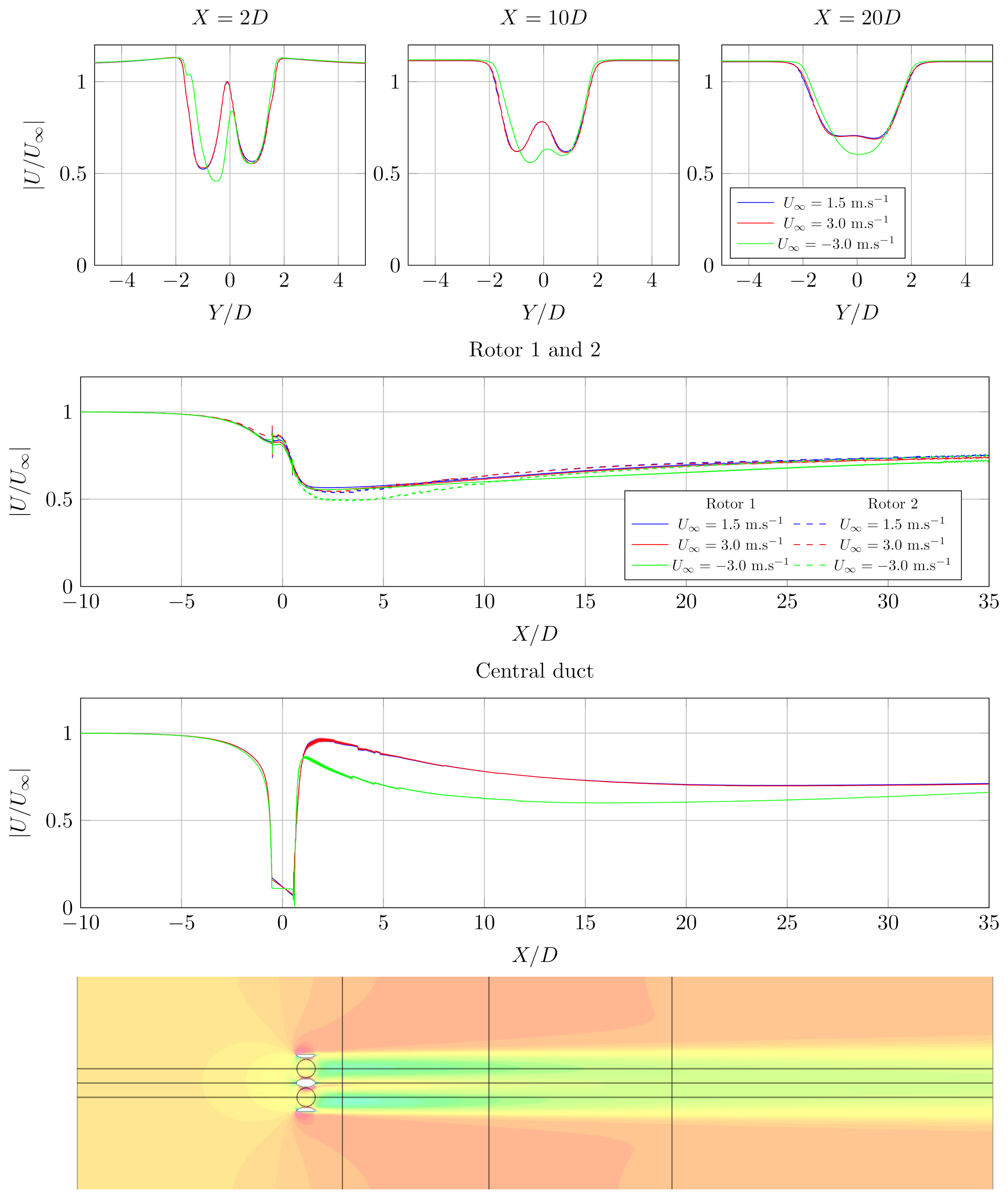
3.2.1. First Farm Configuration

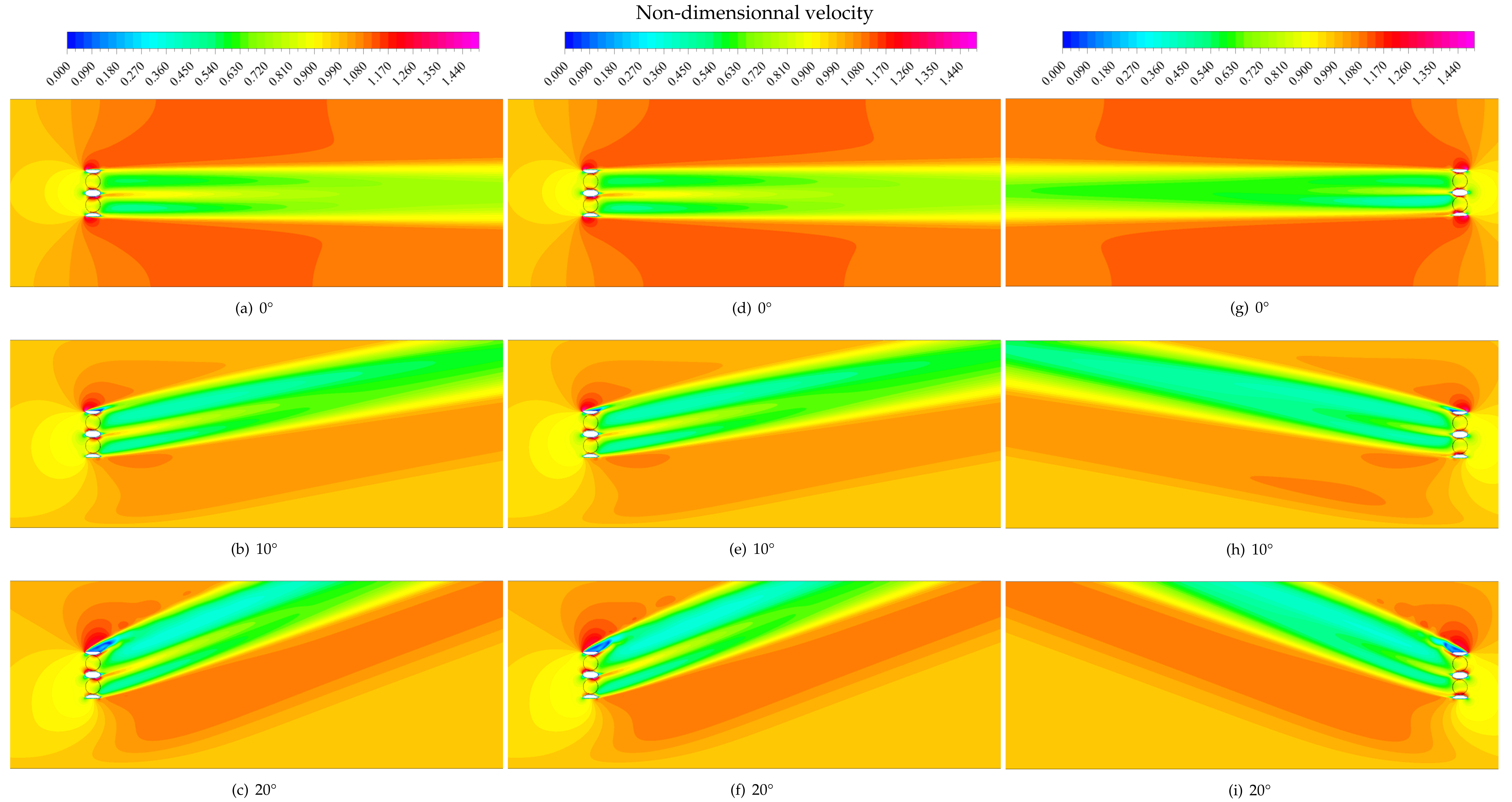
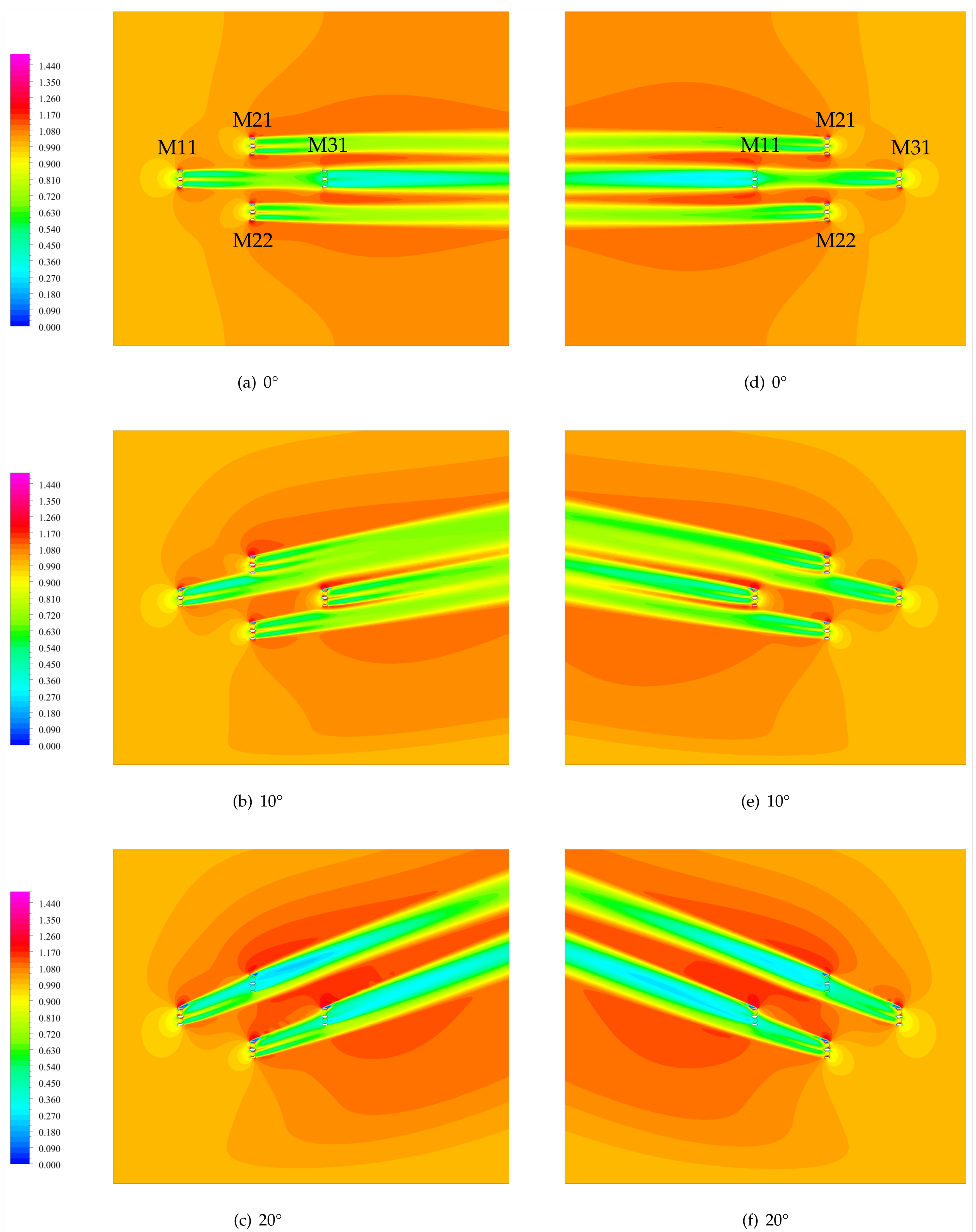
Fields of adimensional velocity for the first configuration and all flow cases are presented in Figure 12. Power production is detailed in Table 4.
As for the single turbine case, rotor 2 produces more than rotor 1, as was found in the single turbine case. However, production for M11 is not the same as production for the single turbine for U = ± 3.0 m · s 1 and γ = 0   . This difference can be explained by a more important global blockage effect for the single turbine, as the inlet surface is less wide than for the farm case. Indeed, blockage correction for a vertical axis-turbine can be expressed by Equation (6) [24,25].
ε = 1 4 A f A t ,
where A f = 25 × H t   m 2 is the total projected area of the turbine, ducts included, and A t the canal inlet surface. For the single turbine, A t = 100 × H t   m 2 , and, for the farm, A t = 500 × H t   m 2 . H t is the turbine height, with approximately 11 m ducts included. In Reference [25], velocity is corrected according to V c o r = V u n c o r 1 + ε ( V c o r is the corrected velocity and V u n c o r the initial velocity uncorrected), resulting in the corrected pressure equation P c o r = P 1 + ε 3 . According to those two formulas, the ratio between power produced by a single turbine and turbine M11 within the farm, the ratio P M 11 P t u r b = 0.920 is almost equal to the ratio of the corrected pressure 1 + ε M 11 3 1 + ε t u r b 3 = 0.865 for the rotor 1. Different blockage effects between the single turbine and M11 in the farm can then explained the difference in power production for the same flow condition at the inlet.
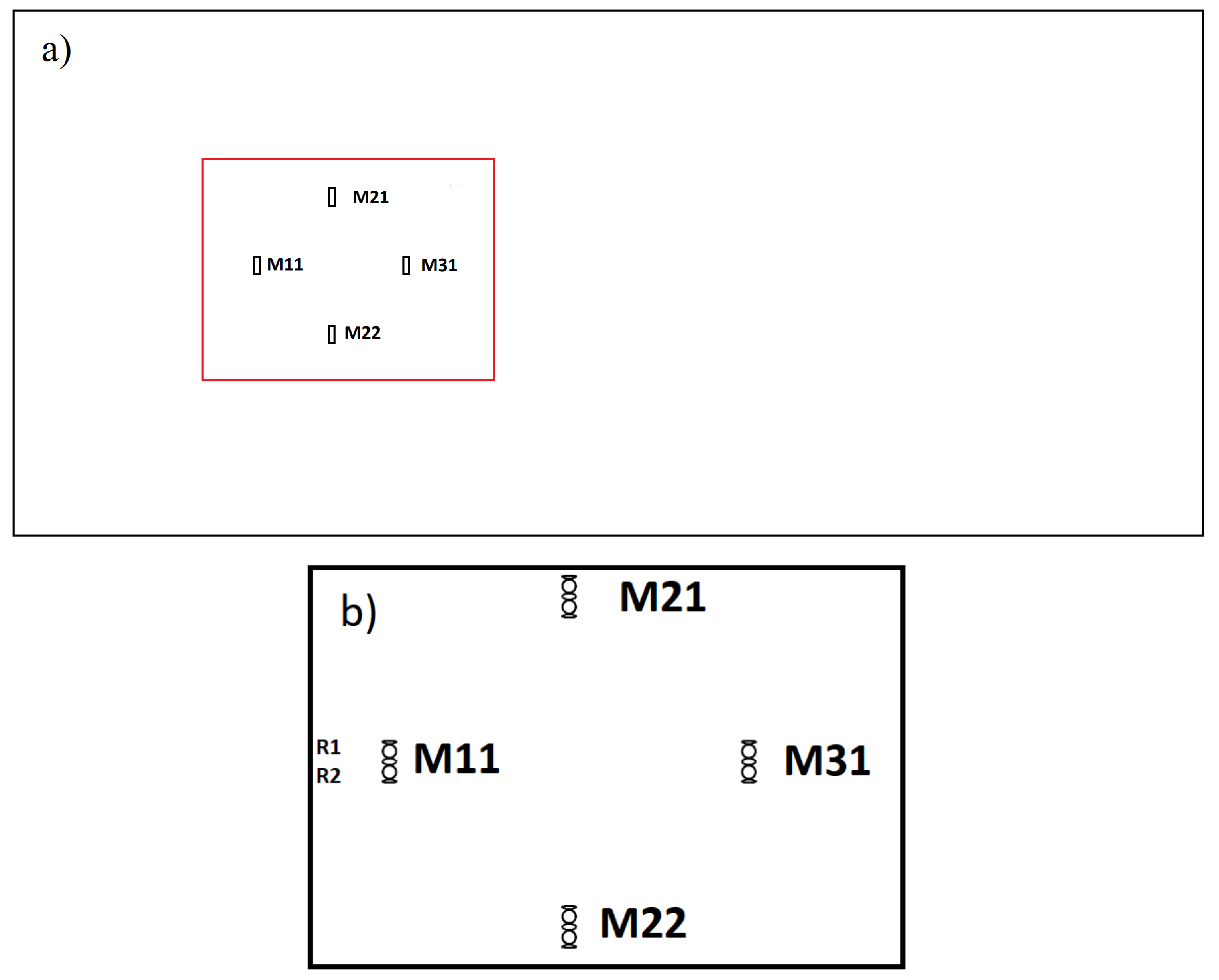
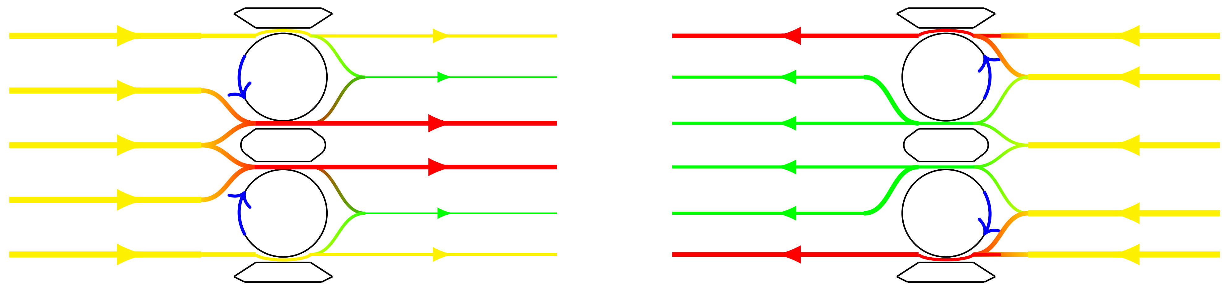
For a case without incidence of the flow (Figure 12a), as M31 is located directly behind M11 (tandem configuration), it suffers from the velocity deficit induced by M11. As a consequence, the inlet velocity of M31 is significantly lower than the upstream velocity, resulting in an even more pronounced wake and, therefore, in a drop of power production (Table 4). In Table 4 and Table 5, power produced by M31, when velocity is positive, is subsequently lower than for the other machines, of almost 40. Same results are encountered upon M11 when the velocity is negative. However, for a negative velocity, production decrease for the last machine relative to the head machine is less pronounced than for a positive velocity. It is most likely due to the fact that the power produced by the head machine is less important in the case of a flow coming backward. M31’s lower power production is likely due to the rotor rotation direction, designed to produce more in a case of a positive velocity.
Turbines on the second rows, i.e., M21 and M22, are not influenced by the M11 velocity deficit; however, looking at velocity fields in Figure 12a,d, it seems that they are slightly impacted by the presence of M11. Looking at adimensional power production in Table 5, it appears that, for a positive velocity, M21 and M22 produce less than the first turbine, of more than 10% for M22’s rotor 2. However, for U < 0 , an inverse effect takes place, and second row turbines produce relatively more than the head turbine. This is likely due to the rotor rotation direction, in which the head machine tends to accelerate flow at its lateral side for a negative velocity, which benefits M21 and M22; for a flow coming inwards, rotors of the first machine tend to bring the flow in the center of the turbine (Figure 13).
In this way, even if the head turbine produces less when the velocity is negative, it induced beneficial effects upon downstream turbines that boost their power production. Consequently, flow acceleration produced by M31 for a negative velocity counterbalances the lower production of M31. Yet, the farm produces less for a negative velocity than a positive one for a straight flow.
For γ = 10   (Figure 12b,e), M31 and M11 are not more in tandem configuration, but yet, found themselves almost in overlapping wake configuration. First, for both velocities, the wake of the head machine seems to be affected by the presence of the tail machine, which results in a shrunk wake and a lower velocity deficit for the first turbine. Furthermore, the last turbine takes advantage of flow acceleration induced by the upstream, resulting in a greater power production relative to the first machine. For a negative velocity, M11 production grows more than 20% (Table 5) for both rotors, with rotor 2 producing more; for a positive velocity, only M31’s rotor 1 takes advantage of the configuration and produces a little more (2%) than M11. Smaller production increase of rotor 1 for U < 0 is justified by the fact that it is more affected by velocity deficit induced by the head machine, and that rotor 2 is more likely to benefit flow acceleration from the head machine and from M22. On the contrary, for a single turbine (Table 3), power production increases as flow incidence reaches 10 . Turbines M21 and M22 also seem to be affected by the presence of the last turbine, as their wakes are a bit less wide too, but to a lesser extent than for turbine M11. Concerning their power productions (Table 4), M21 production increases for an incidence angle of 10 , as does rotor 1 for M22; however, rotor 2 produces less for that angle than for a straight flow. Looking at velocity fields in Figure 12b,e, this rotor is located farther laterally, and it then may not take much advantages of flow accelerations caused by the head machine. Consequently, production of M22 is lower than the one of the head turbine, whatever the flow direction, whereas, for a negative velocity, M21 has a better production than the first machine, due to the same effect of rotor rotation direction explained before. The total farm production is higher than for γ = 0   degree , for more than 1 M W , mainly due to the fact that turbines of the first and last row are no longer in tandem configuration and that lateral turbines benefits from flow acceleration induced by first machine. On the contrary, for the flow case where γ = 0   , the best production is realized with a negative velocity, which is once again the consequence of rotor rotation direction.
The same effects appear for a flow orientation of 20 (Figure 12c), with almost the same production increase relative to the first turbine, but with an overall production for the farm. Last but not least, vortex appear at the edge of rotor 1 ducts, as it happens for the single turbine.
As a consequence, the total power production of this 4-machine farm configuration is more important when the current is deviated up, reaching its maximum for an incidence angle of 20 , first because the last row machine (M31 or M11 depending on velocity sign) is no longer situated directly in the first row machine wake, and, last but not least, because middle turbines take advantage of accelerated flow caused by the first machine. As can be seen in Table 5, where power is adimensioned by power produced by the head turbine, M21 and M22 tend to produce more (relatively of the first turbine production) in the case where the velocity is negative, whatever the flow incidence. In addition, it is noticed that total production is more important when the flow is entering the farm backward. Indeed, in this case, machines of the second row take advantage of flow acceleration induced by the head machine at its side, as observed in Figure 12. Even if the first machine produces less for a negative velocity (M31) than for a positive velocity (M11) due to the rotation direction of the rotor, this effect is canceled out, and even overstepped, by the lateral flow acceleration it creates, leading to beneficial effects upon downstream turbines and increasing total power production. The last turbine to be reached by the flow also produces relatively more, in the case of a negative turbine.

3.2.2. Second Farm Configuration

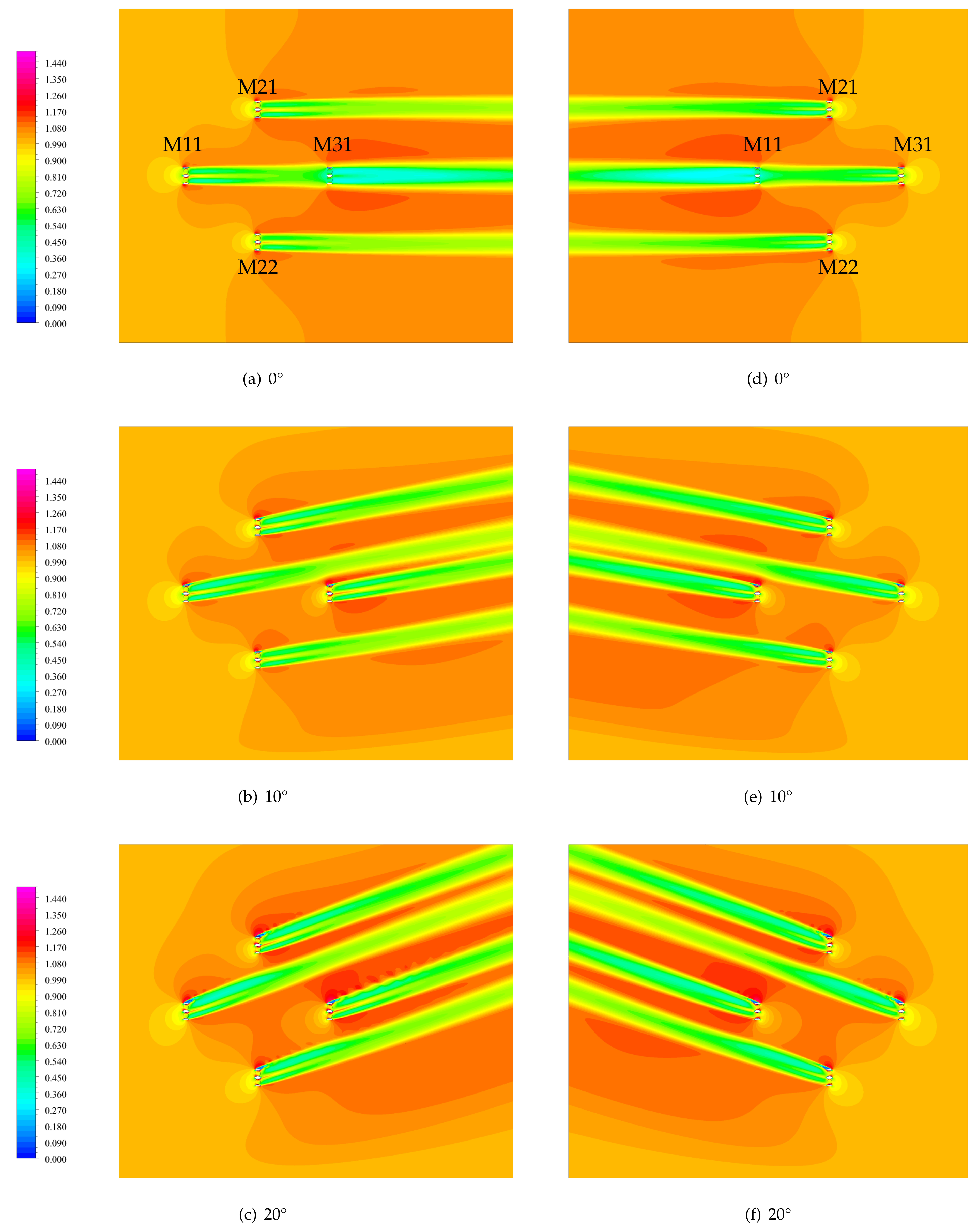
The second farm configuration is tested; the only difference with the first configuration is the lateral distance between turbines, which is here 50 m. In Figure 14 is displayed the adimensional velocity field in the domain for each flow condition at the inlet. Power production and adimensional power production for each case and rotor are detailed, respectively, in Table 6 and Table 7. The power ratio between configuration 2 and 1 for each case is presented in Table 8.
For a straight flow (Figure 14a), the same results on tandem configuration between the first and the last turbines are obtained. Moreover, due to smaller lateral spacing, turbines M21 and M22 have an influence on first and last turbine wakes, which leads to thinner wakes. In the same way, the last turbine interferes with M21 and M22 wakes, resulting in slightly reduced wakes, more noticeable when the velocity is negative. As for the first farm configuration, total production is higher for a negative velocity (Table 6).
Looking at the power ratio between configuration 2 and configuration 1 (Table 8), it appears that turbines produce more than configuration 1, except for M11’s rotor 2 and M21’s rotor 1 for U > 0 and for M31 for U < 0 . For that last case, production of the last machine rotor is 9 and 18 higher for the second configuration; beneficial effects from rotor rotation direction are emphasized with the smaller lateral distancing between turbines. However, for both velocities, total production is only slightly superior for configuration 2.
For γ = 10   (Figure 14b), due to little lateral space between turbines, the last turbines to be reached by the flow (that is to say turbines M21 and M31) found themselves almost in the way of first turbines wakes (configuration of overlapping wakes). Looking at the power production in Table 6 for that current orientation, it seems that turbines M21 and M31 take advantage of flow acceleration caused by first turbines lateral ducts because they tend to produce more than for a straight flow. For U < 0 , M11 and M21 produce, respectively, about 30 and 20 (Table 7) more than the head machine, once again taking advantage of flow acceleration, but at a better extent than for configuration 1, as lateral spacing is reduced. Whatever the velocity, tail turbine and rotor 1 of M21 have a higher power production than for a straight flow. Indeed, rotor 1 of M21 always found itself in the wake of duct-induced flow acceleration. Last, turbines tend to reduce wake of first turbines reached by the flow, for both velocities.
However, when current orientation reaches 20 (Figure 14c), M21 and the last row machine (M31 for U > 0 , M11 for U < 0 ) found themselves directly in tandem configuration with, respectively, head machine and M22. As a result, their production drops drastically compared to an incidence angle of 10 . Rotor 1 of the tail machine seems to suffer less from the upstream velocity deficit (as it produces at least twice as much as rotor 2) because it is located at the edge of the upstream turbine wake. However, M21 is more productive for that flow incidence angle, and rotor 1 always produces more than rotor 2. Indeed, rotor 1 is closer to the first turbine, and it is then more exposed to flow acceleration, increasing its power production. Due to some vortices issued from M22 upper lateral duct, rotor 1 of the last turbine M31 seems to be less affected by velocity deficit, which is confirmed looking at its power production, which is better than for rotor 2. Once again, overall production is higher for a negative velocity.
For this second farm configuration, total power production reaches its maximum for an incidence angle of 10 . On the contrary, for the first configuration, the production is minimal for γ = 20   : incidence angle and lateral distance between turbines are such that they interfere between themselves in a negative way (two tandem configurations).
In Table 8, the ratio of power production of configuration 2 over configuration is detailed. Cells in green indicate a higher production of at least 5 for configuration 2, while red cells illustrate cases where configuration 2 produces at least 5 less than configuration 1.
The first thing obviously noticeable is that there is more red cells than green ones, which means that, when configuration 2 is not as effective as configuration 1, the difference in production is quite important. On the contrary, even if there is more case when configuration 2 produces more than configuration 1, the percentage increase is often not substantial. Indeed, for γ = 0 and 10 , only three rotors of configuration 2 produce less than for configuration 1; but yet, total farm power production is only 1 or 2 higher than for the first configuration. Moreover, production of the second configuration radically drops when the flow incidence angle reaches 20 .
As a consequence, beneficial effects induced by a closer proximity of the turbines are overstepped by negative effects it induced while increasing the flow incidence. The turbines do not take more advantage of flow acceleration induced by head machines, even for a negative velocity, but find themselves in the way of upstream turbines wake, resulting in a extreme power production drop compared to other cases and to head machines.

4. Conclusions

The Actuator Cylinder method was implemented in Ansys Fluent v14.5, resolving the 2D stationary RANS equations, validated, and then applied to the Hydroquest turbine. Turbine and farms were subjected to several flow conditions (orientation and velocity) to evaluate the impact on wake and power production.
During the validation phase, good results were found in efforts representation, as well as wake representation. Both near-wake and its asymmetry and recovery deficit in far-wake were reproduced accurately with the Actuator Cylinder on the Brochier experimental case. First, the case of a single double contra-rotating rotors Hydroquest turbine was considered for different flow conditions in terms of current orientation and velocity (with the same TSR). Consequently, it emerged that current incidence had a slight impact upon power production, and absolute value of velocity had a small influence upon velocity recovery. However, the velocity sign plays an important role for velocity recovery. This could be explained by the operation of the double contra-rotating turbine. Indeed, the flow enters in the turbine by one side during flood and by the opposite side during ebb. In the first case, the flow faces blades going from the outside of the machine to the inside, which was the original feature of the Hydroquest river turbine amplified by specific lateral ducts. During the ebb tide, the flow enters from the back of the machine and sees blades going from the center of the machine to the external side posts.
Different flow orientations, representative of a mean tide in the Alderney Race [16], are then applied for two farm configurations of four turbines, and only lateral spacing differs between the two configurations. As turbines have an impact on the incoming flow, entailing velocity deficit and flow acceleration, they impact production of downstream turbines. Downstream turbines can either take advantage of upstream ones, thanks to the accelerated flows produced by their ducts, or be badly affected, finding themselves in tandem configuration, thus being subjected to weak velocity at their inlet. For both farms, it was observed that production is more important for a negative velocity, except for a straight flow, due to tandem configuration between head and tail turbines. The effects of rotors rotation direction are directly responsible for the higher energy production for a backward flow.
For the first configuration, as lateral distance is quite important, current orientation up to 20 is beneficial for power production more than a non-deviated flow, which is not the case for horizontal-axis turbines [16]. However, for the second configuration, the increase in power production stops at 10 . Indeed, for a higher angle of incidence, two turbines found themselves in tandem configuration, resulting in a drastic drop of power production. In general, configuration 1 produces more than configuration 2, or produces slightly less than configuration 2, depending on current condition. Consequently, considering actual flow current conditions encountered in the Alderney Race, configuration 1 seems to be more appropriate.
Finally, additional investigations and simulations are required to better represent wakes and to predict power production. Hence, some 3D effects can be included, such as the turbine height according to flow height or production of turbulence, which are not taken into account while running 2D simulations. Special attention will be paid to the implementation of a source term for accounting for the turbulence production across the turbine. Farms configurations with more turbines will be studied. Moreover, a statistical approach of the velocity in terms of magnitude and direction in relation with the Actuator cylinder should extend the method to real places, such as the Alderney Race.

Author Contributions

Software, L.J., S.S.G.; validation, L.J.; writing—original draft preparation, L.J.; writing—review and editing, L.J., S.S.G.; supervision, S.S.G.; project administration, S.S.G.; funding acquisition, S.S.G. All authors have read and agreed to the published version of the manuscript.

Funding

This research was funded by Agence de l’Environnement et de la Maîtrise de l’Energie grant number 1682C0085 (OCEANQUEST Project) and Conseil Régional de Normandie grant number 17E01557.

Institutional Review Board Statement

Not applicable.

Informed Consent Statement

Not applicable.

Data Availability Statement

Not applicable.

Acknowledgments

This work was funded by l’Agence de l’Environnement et de la Maîtrise de l’Energie (ADEME) [26] in the frame of the OCEANQUEST project. Computational resources were provided by the Manche county council. The authors would like to thank Hydroquest [27] for the data provided concerning the Hydroquest/CMN tidal turbine.

Conflicts of Interest

The authors declare no conflict of interest.

Nomenclature

A f projected area of the turbine
A t inlet area of the domain
Cblade chord
C D , C L drag and lift coefficients of the blade
Drotor diameter
( e L , e D ) lift and drag forces coordinates system
( e N , e T ) blade coordinates system
( e X , e Y ) Cartesian coordinates system
Ftotal force on the blade
F D , F L drag and lift forces
F N , F T normal and tangential forces
H t rotor height
Nrotor’s number of blades
Ppower production
P c o r , P u n c o r corrected and uncorrected pressure
qintensity of kinetic energy fluctuation
Rrotor radius
Uvelocity
U inlet velocity
Wrelative flow velocity, W = U ω R e T
Xlongitudinal distance downstream from the center of the turbine
Ylateral distance from the center of the turbine
α angle of attack
γ current orientation relative to the X axis
Δ x maximal cells size
ε blockage coefficient for vertical-axis turbine
λ tip speed ratio, λ = ω R U
ρ fluid density
ω rotor rotational velocity

References

  1. Agence de l’Environnement et de la Maîtrise de l’Énergie (ADEME). Étude Stratégique de la FilièRe Hydrolien Marin. Technical Report. Available online: https://librairie.ademe.fr/energies-renouvelables-reseaux-et-stockage/3624-etude-strategique-de-la-filiere-hydrolien-marin.html (accessed on 5 November 2020).
  2. Nguyen, V.; Guillou, S.S.; Thiébot, J.; Santa Cruz, A. A methodology for representing the effect of vertical-axis turbines on the flow. In Proceedings of the 2nd International Conference on Offshore Renewable Energy, Glasgow, UK, 12–14 September 2016. [Google Scholar]
  3. Thiébaut, M.; Sentchev, A.; Bailly du Bois, P. Merging velocity measurements and modeling to improve understanding of tidal stream resource in Alderney Race. Energy 2019, 178, 460–470. [Google Scholar] [CrossRef] [Green Version]
  4. Bahaj, A.; Myers, L. Analytical estimates of the Energy Yield Potential from the Alderney Race (Channel Islands) Using Marine Current Energy Converters. Renew. Energy 2004, 29, 1931–1945. [Google Scholar] [CrossRef]
  5. Thiébaut, M.; Filipot, J.F.; Maisondieu, C.; Damblans, G.; Jochum, C.; Kilcher, L.; Guillou, S. Characterization of the vertical evolution of the three-dimensional turbulence for fatigue design of tidal turbines. Philos. Trans. R. Soc. Math. Phys. Eng. Sci. 2020, 378, 20190495. [Google Scholar] [CrossRef]
  6. Thiébaut, M.; Filipot, J.; Maisondieu, C.; Damblans, G.; Duarte, R.; Droniou, E.; Chaplain, N.; Guillou, S. A comprehensive assessment of turbulence at a tidal-stream energy site influenced by wind-generated ocean waves. Energy 2019, 191, 116550. [Google Scholar] [CrossRef]
  7. Strickland, J.H.; Webster, B.T.; Nguyen, T.A. Vortex Model of the Darrieus Turbine: An Analytical and Experimental Study. Trans. ASME J. Fluids Eng. 1979, 101, 500–505. [Google Scholar] [CrossRef]
  8. Templin, R.J. Aerodynamic Performance Theory of the NRC Vertical Axis Wind Turbine; Technical Report LTR-LA-160; National Research Council of Canada: Ottawa, ON, Canada, 1973. [Google Scholar]
  9. Strickland, J. The Darrieus Turbine: A Performance Prediction Model Using Multiple Streamtubes; Technical Report SAND-75-0431; Sandia Laboratory: Albuberque, NM, USA, 1975. [Google Scholar]
  10. Paraschivoiu, I. Aerodynamic Loads and Performance of the Darrieus Turbine. Am. Inst. Aeronaut. Astronaut. J. Energy 1981, 6, 406–412. [Google Scholar]
  11. Poguluri, S.K.; Lee, H.; Bae, Y.H. An investigation on the aerodynamic performance of a co-axial contra-rotating vertical-axis wind turbine. Energy 2021, 219, 119547. [Google Scholar] [CrossRef]
  12. Shamsoddin, S.; Porté-Agel, F. Large Eddy Simulation of Vertical Axis Wind Turbine Wakes. Energies 2014, 7, 890–912. [Google Scholar] [CrossRef]
  13. Grondeau, M.; Guillou, S.; Mercier, P.; Poizot, E. Wake of a Ducted Vertical Axis Tidal Turbine in Turbulent Flows, LBM Actuator-Line Approach. Energies 2019, 12, 497–512. [Google Scholar] [CrossRef] [Green Version]
  14. Dabiri, J. Potential order-of-magnitude enhancement of wind farm power density via counter-rotating vertical-axis wind turbine arrays. J. Renew. Sustain. Energy 2011, 3, 043104. [Google Scholar] [CrossRef] [Green Version]
  15. Palm, M.; Huijsmans, R.; Pourquie, M. The Applicability of Semi-Empirical Wake Models for Tidal Farms. In Proceedings of the European Wave and Tidal Energy Conference, Southampton, UK, 5–9 September 2011. [Google Scholar]
  16. Nguyen, V.T.; Santa Cruz, A.; Guillou, S.; Shiek Elsouk, M.; Thiébot, J. Effects of the Current Direction on the Energy Production of a Tidal Farm: The Case of Raz Blanchard (France). Energies 2019, 12, 2478. [Google Scholar] [CrossRef] [Green Version]
  17. Clary, V.; Oudart, T.; Larroudé, P.; Sommeria, J.; Maître, T. An optimally-controlled RANS Actuator force model for different computations of tidal turbine arrays. Ocean. Eng. 2020, 212, 107677. [Google Scholar] [CrossRef]
  18. Madsen, H.A. The Actuator Cylinder—A Flow Model for Vertical Axis Wind Turbines. Ph.D. Thesis, Aalborg University Centre, Aalborg, Denmark, 1982. [Google Scholar]
  19. Sheldahl, R.; Klimas, P. Aerodynamic Characteristics of Seven Symmetrical Airfoil Sections through 180-Degree Angle of Attack for Use in Aerodynamic Analysis of Vertical Axis Wind Turbines; Technical Report SAND-80-2114; Sandia Laboratory: Albuquerque, NM, USA, 1981. [Google Scholar]
  20. Brochier, G. Étude Numérique de la Couche Limite Instationnaire sur un Profil d’Aile en Mouvement, Application et Expérimentation à l’Éolienne Darrieus. Ph.D. Thesis, Université d’Aix-Marseille II, Marseille, France, 1986. [Google Scholar]
  21. Nguyen, V.T.; Guillou, S.S.; Thiébot, J.; Santa Cruz, A. Modelling turbulence with an Actuator Disk representing a tidal turbine. Renew. Energy 2016, 97, 625–635. [Google Scholar] [CrossRef]
  22. Maitre, T.; Amet, E.; Pellone, C. Modeling of the flow in a Darrieus water turbine: Wall grid refinement analysis and comparison with experiments. Renew. Energy 2012, 51, 497–512. [Google Scholar] [CrossRef]
  23. Howell, R.; Qin, N.; Edwards, J.; Durrani, N. Wind tunnel and numerical study of a small vertical axis wind turbine. Renew. Energy 2009, 35, 412–422. [Google Scholar] [CrossRef] [Green Version]
  24. Hilewit, D.; Matida, E.; Fereidooni, A.; Aboel Ella, H.; Nitzsche, F. Power coefficient measurements of a novel vertical axis wind turbine. Energy Sci. Eng. 2019, 7, 2373–2382. [Google Scholar] [CrossRef]
  25. Ross, I. Wind Tunnel Blockage Corrections: An Application to Vertical-Axis Wind Turbines. Master’s Thesis, School of Engineering of the University of Dayton, Dayton, OH, USA, 2010. [Google Scholar]
  26. Agence de l’Environnement et de la Maîtrise de l’Énergie (ADEME). Available online: www.ademe.fr (accessed on 5 November 2020).
  27. Hydroquest. Available online: www.hydroquest.fr (accessed on 5 November 2020).
Figure 1. Hydroquest turbine with its anchorage.
Energies 14 05199 g001
Figure 2. Actuator Cylinder model scheme: The rotor is represented as a hollow cylinder which external and internal radius are determined by the blade path.
Energies 14 05199 g002
Figure 3. Normal (left) and tangential (right) forces in function of the azimuthal position θ , comparison between the experience of Strickland for three blades and the numerical results of Nguyen et al. [2].
Energies 14 05199 g003
Figure 4. Transverse profiles of adimensional velocity U / U and intensity of kinetic energy fluctuation q / U downstream the turbine; X represents the distance downstream (black lines on the velocity field figure).
Energies 14 05199 g004
Figure 5. Hydroquest tidal turbine prototype before installation in Paimpol-Bréhat test site.
Energies 14 05199 g005
Figure 6. Meshed turbine and tunnel on Ansys Meshing: (a) Mesh around the turbine; (b) Mesh inflation around the rotor cylinder.
Energies 14 05199 g006
Figure 7. Computational domain for the single turbine; center of the domain is located at the center of the central duct of the turbine.
Energies 14 05199 g007
Figure 8. Mesh convergence test in terms of adimensional velocity profiles (see probes location in Figure 9).
Energies 14 05199 g008
Figure 9. Transverse and longitudinal profiles of adimensional velocity intensity in the wake of the Hydroquest turbine for γ = 0 ; probes locations at the upstream distance X from the turbine center are shown in black lines.
Energies 14 05199 g009
Figure 10. Turbines arrangement within the farm (a) with turbines name; zoom near the four turbines (b).
Energies 14 05199 g010
Figure 11. Flow around a single turbine: Non-dimensional velocity ( U a = U / U ) field for U = 1.5 m · s 1 , (ac), U = 3.0 m · s 1 (df), and U = −3.0 m · s 1 , (gi).
Energies 14 05199 g011
Figure 12. Non-dimensional velocity ( U a = U / U ) field for the first farm configuration: U > 0 on the left side, and U < 0 on the right side.
Energies 14 05199 g012
Figure 13. Flow acceleration depending on the velocity sign, in the case of a flow over a single turbine (positive velocity on the left, negative velocity on the right; red lines indicate an accelerated flow, and green lines indicate a decelerated flow).
Energies 14 05199 g013
Figure 14. Non-dimensional velocity ( U a = U / U ) field for the second farm configuration: U > 0 on the left side, and U < 0 on the right side.
Energies 14 05199 g014
Table 1. Characteristics of Strickland experiments.
CharacteristicValueUnit
Rotor radius0.061 m
Blade number1, 2, and 3-
Blade profileNACA 0012-
Chord0.0914 m
Inlet velocity0.091m · s −1
TSR5-
Table 2. Characteristics of the Brochier experiment.
CharacteristicValueUnit
Rotor radius0.06 m
Blade number2-
Blade profileNACA 0018-
Chords0.02 m
Inlet velocity0.02m · s −1
Turbulent intensity5%
TSR3.85-
Rotation speed83 tr / min
Table 3. Power production ( M W ) for each rotor for different flow conditions.
Velocity U = 1.5 m · s 1 U = 3 m · s 1 U = −3 m · s 1
IncidenceRotor 1Rotor 2Rotor 1Rotor 2Rotor 1Rotor 2
γ =   0 0.0800.0920.6500.7450.6500.745
γ =   10 0.0790.0810.6320.6440.6480.674
γ =   20 0.0880.0830.7060.6620.6930.701
Table 4. Power produced ( M W ) by every rotors of every turbines in the first farm configuration for the different flow conditions tested.
MachineM11M21M22M31 P tot
Case Rotor 1Rotor 2Rotor 1Rotor 2Rotor 1Rotor 2Rotor 1Rotor 2
γ = 0∘ U > 0 0.5720.7110.5610.6700.5210.6250.2320.2454.137
U < 0 0.2290.2370.5720.6610.5730.6000.5440.5884.004
γ = 10∘ U > 0 0.6550.7150.6370.6820.5500.6080.6700.7115.228
U < 0 0.7740.7880.6470.6980.6080.5980.6300.6175.360
γ = 20∘ U > 0 0.7320.7130.7270.7560.6470.6280.7410.7695.713
U < 0 0.8470.8340.7360.7630.6720.6390.6910.6595.841
Table 5. Adimensional power produced by every rotors of every turbines in the first farm configuration for the different flow conditions tested, adimensioned by the header turbine (M11 for a U > 0 , M31 for U < 0 ).
MachineM11M21M22M31
Case Rotor 1Rotor 2Rotor 1Rotor 2Rotor 1Rotor 2Rotor 1Rotor 2
γ = 0∘ U > 0 1.001.000.980.940.910.880.410.34
U < 0 0.420.401.051.121.051.021.001.00
γ = 10∘ U > 0 1.001.000.970.950.840.851.020.99
U < 0 1.231.281.031.130.970.971.001.00
γ = 20∘ U > 0 1.001.000.991.060.880.881.011.08
U < 0 1.231.271.071.160.970.971.001.00
Table 6. Power produced ( M W ) by every rotor of every turbine in the second farm configuration for the different flow conditions tested.
MachineM11M21M22M31 P tot
Case Rotor 1Rotor 2Rotor 1Rotor 2Rotor 1Rotor 2Rotor 1Rotor 2
γ = 0∘ U > 0 0.5890.6450.5720.6840.5470.6470.2220.2594.165
U < 0 0.2490.2790.5760.6820.6000.6600.5080.5464.100
γ = 10∘ U > 0 0.6770.6820.6350.6790.5960.6290.6760.7185.292
U < 0 0.7750.8090.6580.7300.6170.6250.5680.6115.474
γ = 20∘ U > 0 0.7290.6790.1700.1300.6580.6490.4300.1683.613
U < 0 0.5430.2000.2150.1610.6790.6400.6180.6423.698
Table 7. Adimensional power produced by every rotors of every turbines in the second farm configuration for the different flow conditions tested, adimensioned by the header turbine.
MachineM11M21M22M31
Case Rotor 1Rotor 2Rotor 1Rotor 2Rotor 1Rotor 2Rotor 1Rotor 2
γ = 0∘ U > 0 1.001.000.971.060.931.000.380.40
U < 0 0.490.511.131.251.181.211.001.00
γ = 10∘ U > 0 1.001.000.941.000.880.921.001.05
U < 0 1.361.321.161.191.091.021.001.00
γ = 20∘ U > 0 1.001.000.230.190.900.960.590.25
U < 0 0.880.310.350.251.101.001.001.00
Table 8. Ratio of power production of second configuration over first configuration; cells in red show that configuration 2 produces at least  5 less than configuration 1, and cells in green that power produced by configuration 2 is at least  5 more than configuration 1.
MachineM11M21M22M31 P tot
Case Rotor 1Rotor 2Rotor 1Rotor 2Rotor 1Rotor 2Rotor 1Rotor 2
γ = 0∘ U > 0 1.030.911.021.021.051.040.961.061.01
U < 0 1.091.181.011.031.051.100.930.931.02
γ = 10∘ U > 0 1.030.951.001.001.081.031.011.011.01
U < 0 1.001.031.021.051.011.050.900.991.01
γ = 20∘ U > 0 1.000.950.230.171.021.030.580.220.63
U < 0 0.640.240.290.211.011.000.890.970.63
Publisher’s Note: MDPI stays neutral with regard to jurisdictional claims in published maps and institutional affiliations.

