1. Introduction
The traditional way of energy harvesting is inefficient and emission-intensive, which is the culprit for global climate change, extreme weather, and natural disasters. Therefore, the trend to use new environmentally friendly energy resources instead of traditional energy resources is becoming prosperous [
1]. Renewable resources such as solar energy, fuel cells, and wind energy are introduced into the energy market as distributed generation (DG) in order to combat greenhouse gas emission. To explore the full potential of renewable energy, a microgrid is proposed to coordinate these distributed energy resources (DER) and renewable energy storage systems (RES) with different loads [
2,
3,
4,
5], which can operate either in grid-connected mode or isolated mode [
6]. Furthermore, the isolated microgrid, also called an islanded microgrid, plays a vital role in supplying power in rural areas and sparse locations.
Recently, the multi-energy microgrids are growing prosperously. Different energy sources are incorporated into this multi-engergy microgrid [
7,
8]. It usually includes an electric system, natural gas, and hydrogen. This multi-energy system has higher efficiency than the singe source as the different energy sources in the system can compensate each other [
7]. Further, multi-energy systems with more than two different source are gaining more attention as well. The DC microgrid is able to interface DERs, RES, and loads into one common bus, which is becoming much more attractive worldwide. Compared to the AC microgrid, the DC microgrid is more efficient due to its less energy-consuming conversion process which leads to less heat waste [
9,
10]. There is also no synchronization involved for the DC microgrid, which simplifies the control and optimization process. Furthermore, some disadvantages the AC microgrid has can be conquered by a DC microgrid, such as power quality enhancement, inrush current of transformer, and reactive power flow [
11]. Owing to the RES’ utilization, the blackout influence from the primary grid is negligible [
1]. Especially for remote areas which are geographically isolated, an independent power source is essential. The independent DC power systems are called islanded DC microgrids [
12], and they can reliably provide electricity supply at critical loads [
2].
To safeguard DC microgrid operation and promote its widespread installation [
13], a comprehensive and well-functioning protection method could drastically increase the reliability, dependability, and security of DC microgrid [
14,
15]. However, one of the main challenges for DC microgrid protection is detecting fault without the natural zero-crossing point [
10,
16,
17]. In addition, due to the low cable resistance, the fault current increases rapidly, making protection coordination more difficult. To address above challenges, one of the solutions is artificial intelligent based method, which has been drawn attention recently in DC microgrids [
18,
19,
20,
21,
22]. Although these intelligent methods have been demonstrating promising results, there are still many technical barriers preventing them from being applied to industry such as limited/imbalanced dataset, data inconsistency, and difficulties in cost-effective real-time implementation.
Until now, many protection methods have been studied for DC microgrid. Similar to the AC microgrid, overcurrent protection, differential protection, directional overcurrent protection, distance protection, and current derivative protection methods have gained much attention [
16]. A protection method for the DC ring bus system is described in [
23], which is based on the parameters measured locally. Distance protection can be applied to DC microgrids as well. The distance information can be obtained by measuring from the checking point to the faulty point. If the value of impedance falls into the operation zone, the fault will be detected. In [
24], the local measurement-based method was utilized to protect the DC microgrids as well. The integral and derivative of current values are used to detect the fault. In [
25], Yang et al. proposed a method by analyzing circuit and adopting iteration calculation. However, the error is dependent on the fault resistance, which reduces the reliability of this algorithm. The impedance between the checking point and the faulty point can also be measured by employing the filters and extra sensors, which was discussed in [
26]. It can avoid weakness of a communication system. However, the cost of this method is relatively high compared to the method proposed in [
25]. As for the high impedance and a small part of the cable, this method has lower accuracy. Jia et al. in [
27] discussed a new back-up protection method using transient current correlation to set the threshold.
Overcurrent-based protection strategies and differential protection strategies are the main choices for the DC microgrid [
28]. In [
29,
30], differential protection methods by measuring the current on each side of the feeder had been discussed. A protection method using differential protection and discrete wavelet transform was proposed in [
31]. However, the synchronization and communication between the measurement unit and the control center may lead to the data transfer delay. In [
32], Reis et al. discussed the current derivative-based protection method. This method is based on the increasing speed of the fault current. Augustine et al. in [
33] proposed current derivative protection combined with adaptive droop control to lower the fault current and explain the way to define the current derivative threshold. Compared to other overcurrent-based protection methods, more sensors with high sampling frequency need to be installed in the microgrid, which significantly increases the noise and possibilities to get maltrip. Moreover, the threshold for the high current derivative is also difficult to be set. Based on the overcurrent protection, both fault current and its direction were considered in [
34,
35]. These kinds of methods demonstrate better selectivity and reliability than overcurrent protection. However, the renewable energy systems that exert significant influence on the DC microgrids were not taken into account in these papers. Most importantly, the detailed way to set the pick-up current threshold was not discussed thoroughly in existing papers, and effective methods are yet to be developed. In [
2,
36], authors proposed overcurrent protection method for DC microgrid. The fault current is compared with the tripping threshold set for detection. When the fault current is over the limit, the overcurrent protection scheme is triggered. However, it is not clear whether this setup is suitable for detecting different types of fault and identifying load changes; they are mainly dependent on the threshold, devices, and architecture, which reduce the robustness of the system. If DC microgrid has a complex architecture, the coordination time would be longer, and the elimination of the fault could cause the large-scale disconnection. It is essentially important for the overcurrent protection to determine the maximum line current accurately to have proper pick-up current setting and such a target has not been fully achieved by the papers reviewed above. Although Shabani et al. in [
28] discussed using maximum line current, the detailed way to acquire the maximum operation current was not fully expressed.
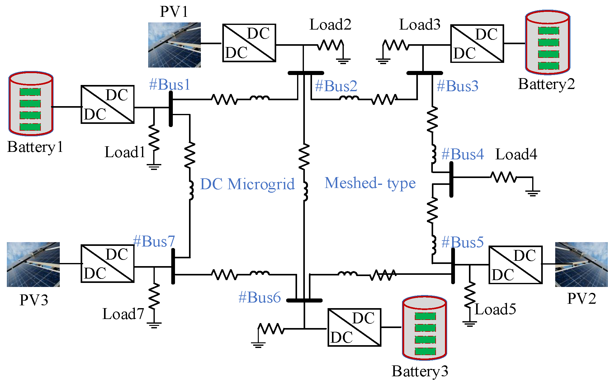
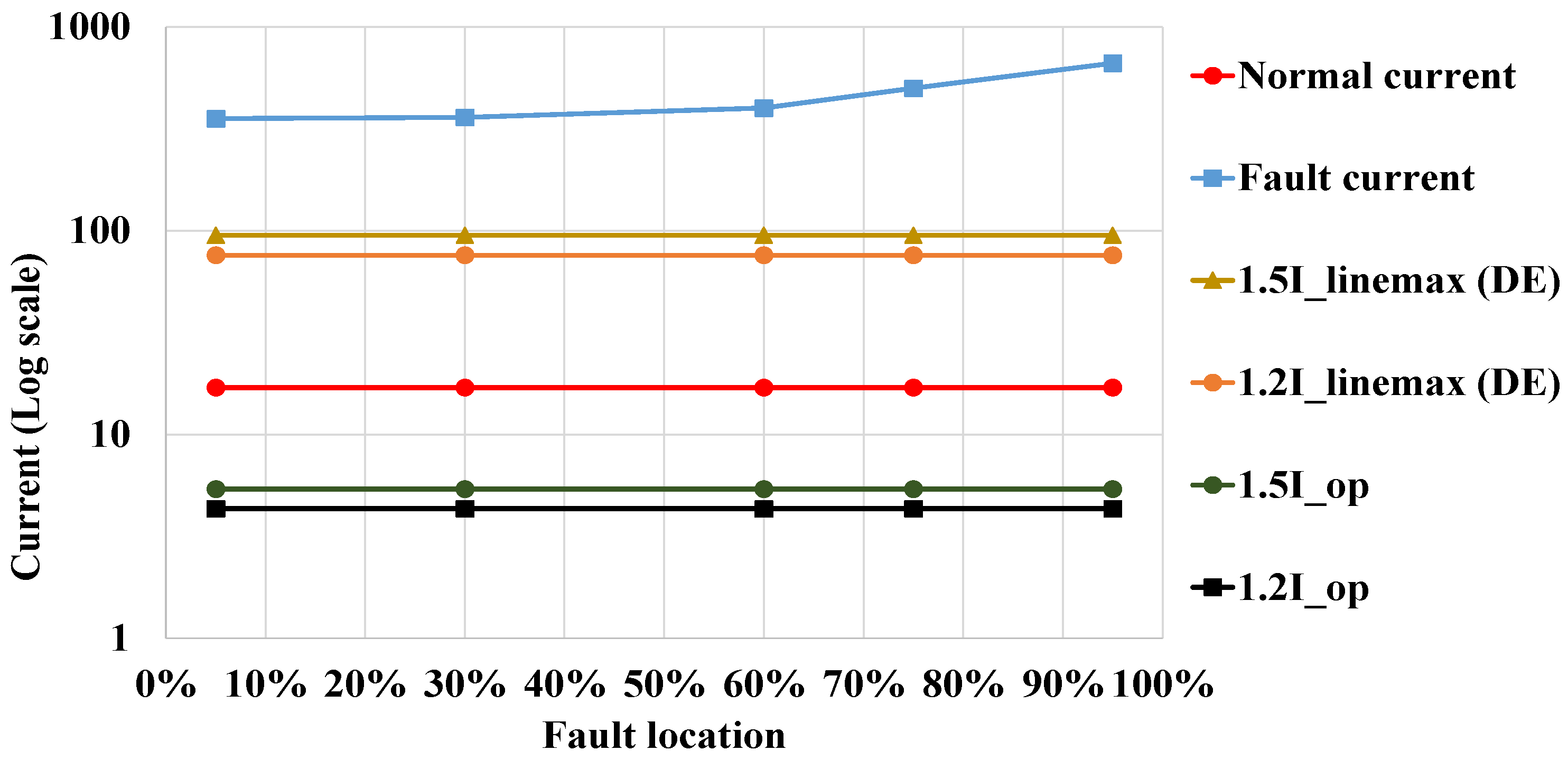
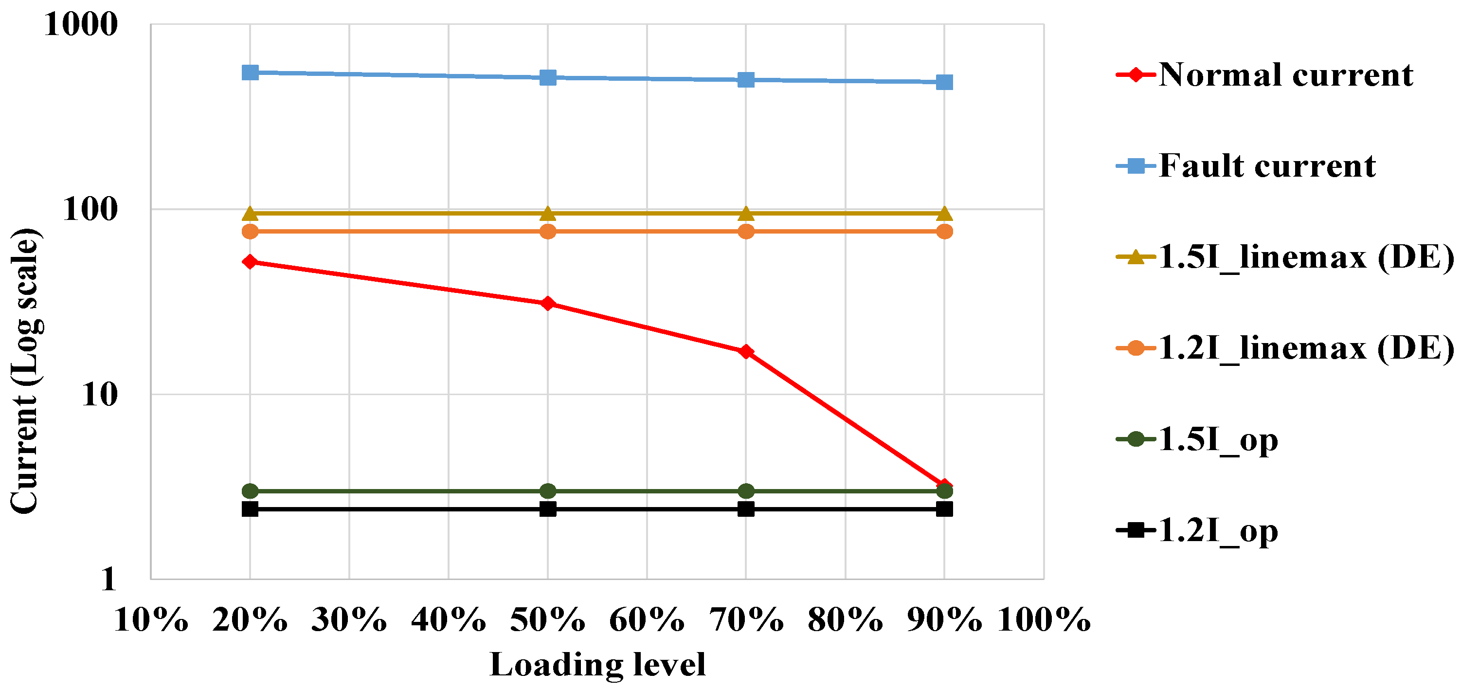
To overcome the difficulties of setting threshold for the overcurrent protection, a novel differential evolution (DE) based framework has been proposed. In this framework, the simplified model has been adopted to simulate the complex model’s steady-state response. Furthermore, the DE algorithm has been first utilized to obtain the maximum line current based on the simplified model. Then, the new way to calculate the pickup current for overcurrent protection has been investigated through a four-bus system with ring configuration. The extendability has been discussed by making use of the seven-bus system with mesh configuration. The proposed framework has been developed after all power resources have been connected to each bus. The black start condition will not be considered in this case.
The remaining parts of the paper are organized with following sequence.
Section 2 discusses the procedure of obtaining the simplified model in great detail. The simplified model and complex model are proven to be consistent in steady state results in
Section 3. At the same time, the extensive case studies have been conducted to validate the feasibility of proposed DE protection framework. Conclusion and remarks on the protection method and the simulation results have been drawn in
Section 4.
2. The Simplified DC Microgrid Model
Instead of simulating the DC microgrid using a complex model, a simplified model is adopted to establish the steady-state analysis for DC microgrids. For different DGs, they can be converted to the simple models separately. Based on the interconnection of the single bus, the whole DC microgrid model can be simplified.
2.1. DC Microgrid System Complex Model Configuration under Conversion
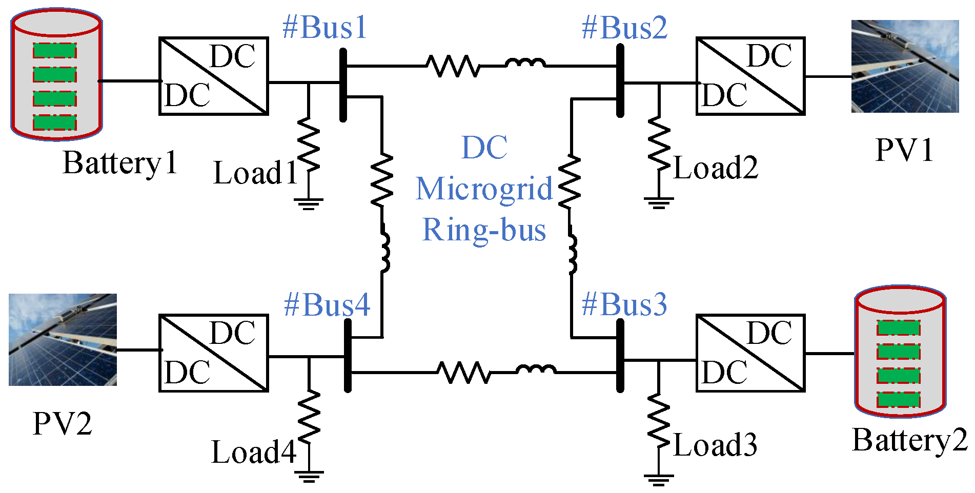
An islanded ring-type DC microgrid is built to design the protection method shown in the
Figure 1. Compared to other topologies, the ring bus topology is a highly reliable [
37]. This DC microgrid contains two Photovoltaic (PV) systems and two battery systems. There are two units in each PV system: PV arrays (modeled by SunPower SPR-305E-WHT-D model provided by Matlab/Simulink) and one bidirectional boost converter. The Perturb and Observe (P&O) control method is adopted to obtain the maximum power. For battery system, it consists of battery units and a boost converter. The parameters for the DC microgrid are summarized in
Table 1. In addition,
Table 2 presents the detailed parameters for the PV array model used in Matlab/Simulink.
2.2. Simplified Model
2.2.1. PV System Model
As discussed in the previous section, the PV system needs to be operated at the maximum power point (MPP), which is affected by varying solar irradiance and temperature [
38]. Thus, a maximum power point tracking (MPPT) technique is applied [
38]. Furthermore, if the operating point is off track, MPPT must quickly react to any unprecedented conditions and regulate the PV system back to MPP.
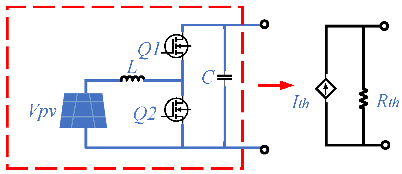
During the conversion process, it is assumed the PV system operates at MPP at all times at a certain irradiance level. The applied voltage control system ensures the PV system’s output voltage is the same as the constant bus voltage. As a result, the output current can be derived from the maximum power and the bus voltage. The expression can be shown as follows:
where
denotes the output current of the PV system,
stands for the total maximum power of the PV system, and
is the DC bus voltage. Considering that the MPP is affected by varying environmental conditions, the PV system output current is regarded as a controlled current source. Thus, PV system output can be simplified as a controlled current source connected in paralleled with a resistance shown in
Figure 2.
in
Figure 2 is the total output equivalent resistance for the PV system.
2.2.2. Battery System Model
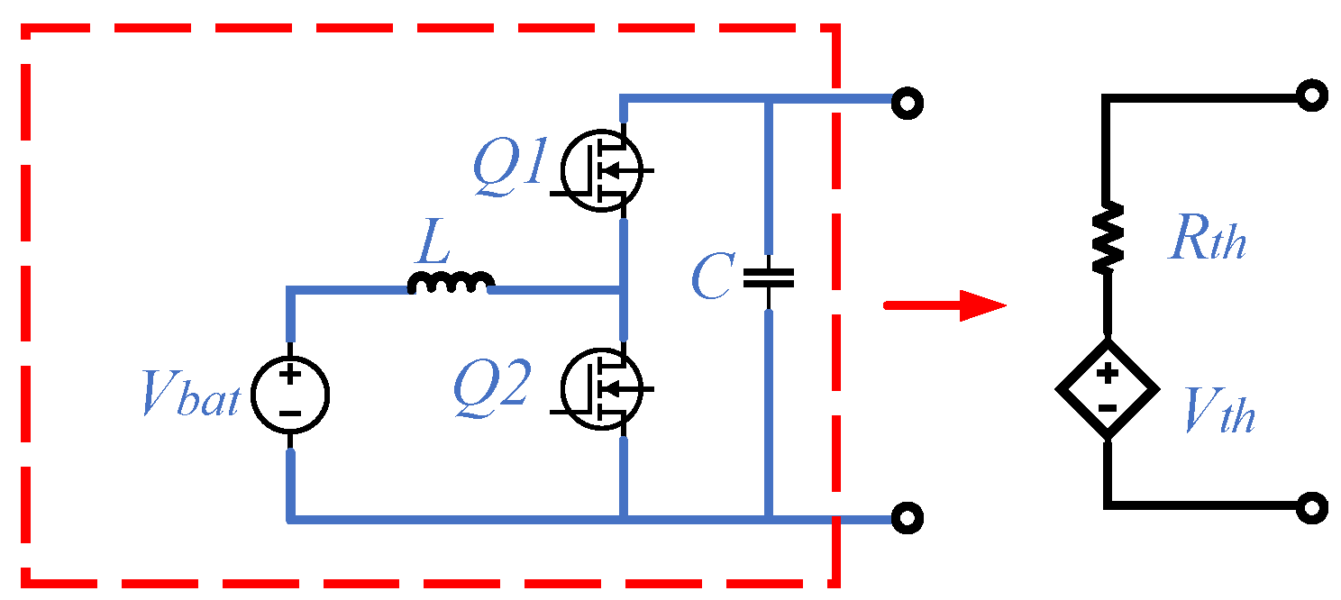
The role of the battery storage system is to keep the DC bus voltage at a certain level, which improves power sharing between different resources. The battery system will inject more power into the microgrid when other resources are not generating enough power to meet the microgrid’s electricity demand. Otherwise, the extra energy generated is diverted into battery system. At the same time, cascade control is used to stabilize the output voltage and output current at a certain level. In addition, droop control is applied to achieve equal power sharing of the batteries, and to distribute power to different battery systems. The droop control used in this paper is voltage droop control. Thus, by combining cascade control with voltage droop control, the battery can be treated equally as a controllable voltage source with an internal resistance shown in
Figure 3. Due to the power sharing function, the output voltage of the battery in
Figure 3 can be expressed by the equation showing below:
where
denotes the terminal voltage of battery system,
denotes the required DC bus voltage,
is the droop coefficient of droop control for each battery system, and
is bus current fed into battery system. In Matlab/Simulink, a controlled voltage source is adopted to represent the simplified battery model. In
Figure 3,
is the total output equivalent resistance of battery system, and
is the output voltage of battery system.
2.3. Current Flow Analysis
In an
N-bus system, there are
x buses with PV systems,
y buses with battery systems, and
pure loads. To analyze the system load flow, it is necessary to obtain the expression for each line current. The line currents can be derived by determining bus voltages by the following matrix:
where
denotes equivalent current source at each bus,
means the admittance matrix of the system and
stands for the bus voltage matrix. For this
N-bus system, the admittance matrix
can be obtained as follows:
The diagonal elements
of the
stand for the self admittance for each node. It can be expressed as
where
stands for the all the self admittance connected to the reference node
i.
denotes the index of nodes. The off-diagonal components
denote the mutual admittance between two nodes
i and
j, and their values should be negative. As shown in
Figure 1, there is a local load connecting to each node, therefore, its contribution to the respective diagonal element can be expressed as
. The diagonal element expression is shown as
Based on the simplified model mentioned in the previous part, a PV system can be simplified as a controlled current source, which means that the output current of the whole PV system is known. The battery system can be evaluated as a controlled voltage source, which defines the output voltage of the battery source. Based on the droop coefficients used, the output voltage of battery system can be derived.
The bus voltage is expressed as Equation (
8):
For the
ith bus voltage, if it is a battery system, the voltage can be expressed as
If the
ith system is a pure load, voltage can be derived as
Furthermore, the bus current can be expressed as
If
ith system is a PV system,
can be revealed as
Taking Equation (
8) to Equation (
12) together, bus voltage can be gained.
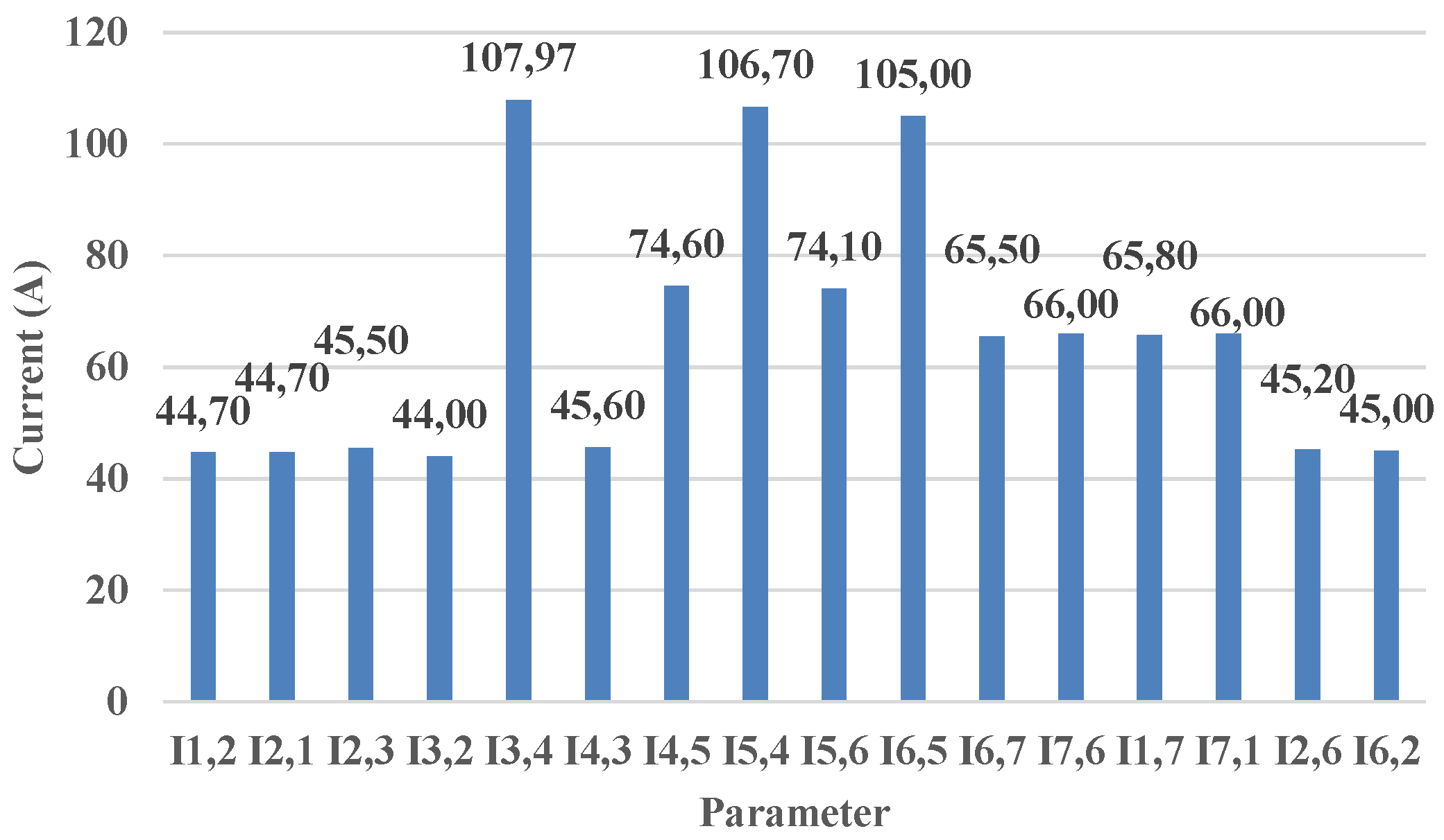
Then, after obtaining the bus voltage, the line current can be calculated as follows:
where
denotes the current flows from bus
i to bus
j. If the current flows from bus
j to bus
i, it can be expressed as
.
2.4. Differential Evolution
DE is one of the most popular optimization methods widely used in different engineering fields [
39], especially in those fields which need to solve stochastic and optimized problems. DE has many advantages that support its popularity, such as simplicity in its codes, lower space complexity, a smaller number of control parameters and its robustness [
40]. The aim of DE is to find out the best parameters under some certain situations with specified constraints.
The number of individual included in the population of DE is
. Each individual can be expressed as vector
X with
D dimensions [
41]:
where
i denotes the solution in
generation,
.
stands for the generations in DE.
The main steps of DE includes initialization, mutation, crossover, and selection. The initialization vectors are randomly defined by some restraints, which usually have their natural limits. The
=
and
are the prescribed minimum and maximum parameter limits. The first vector should contain elements as many as possible, which widens the searching range. Then, the initial
components of
vector at initial generation (
) are defined by
where
stands for the uniformly random distributed parameters and its range is 0 ≤
≤ 1.
After initialization process is completed, the mutation operation starts. The disturbance is added to the target vector. The donor vector can be expressed as follows:
where
,
, and
indicate the random numbers selected among population within the range of [1,
] [
42], and
F is the positive scaling factor aiming to scaling the difference vector [
43].
To enrich the diversity of population, the trial vector
=
has been generated by applying crossover to each pair of the target vector
and its related mutant vector
. The trial vector elements are obtained by extracting variables from
and
.
where
denotes the crossover rate within the range [0, 1) functioning as the scalar control parameters for controlling the fraction of parameter values copied from the mutant vector.
is the
elements of the
choice in generation
G.
is the integer in the range of [1,
D] selected randomly [
43].
The last operation step of DE is selection. The main purpose of selection is to filter unqualified target vector or trial vector to the next generation.
is the objective function to be minimized. Based on following formula, the operation can be conducted [
44].
After the initialization, the iteration operation steps from mutation to selection, and the processing stops until the ceasing criteria has been fulfilled.
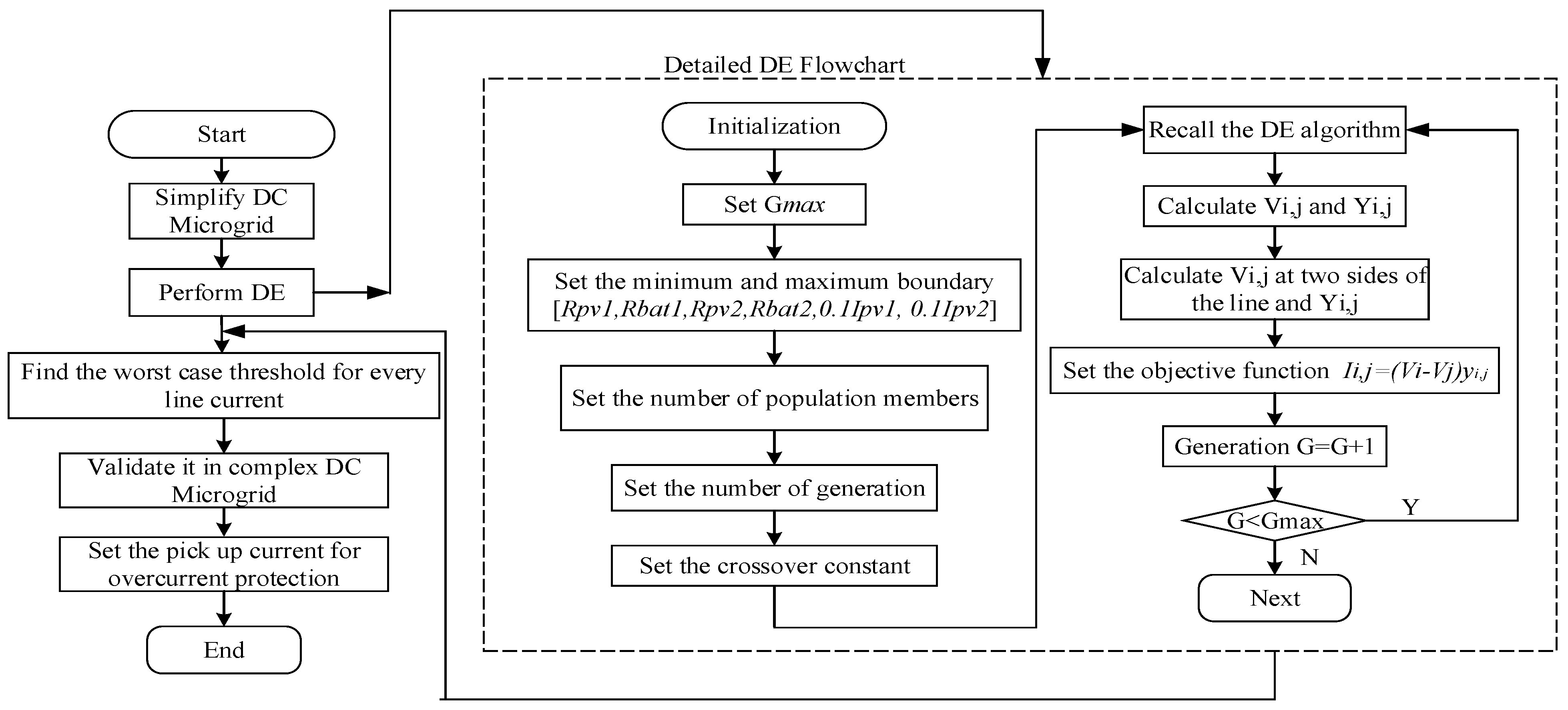
In this paper, the purpose of using DE is to acquire the largest line current. Then, the objective function set for this paper would be = . The aim of the optimization is to minimize the value of . When reaches its smallest value, the value of becomes the largest, which is the required worst case line current value.
The parameters set for the initial population are loads of different systems and output current of PV system. The output current at MPP shows the different irradiance under dissimilar weather conditions. Suppose both PV systems work under MPP due to the effective MPPT method, the lower boundary set for PV irradiance is one-tenth of the maximum irradiance, which corresponds to . denotes PV current under standard test condition which is 25 C, 1000 W/m. 0.1 of simulates the cloudy day which has little sunshine. The upper boundary set for PV irradiance is the maximum irradiance referring to the .
The overall algorithm framework flowchart is shown in the
Figure 4.


