Appendix C. RE Production Calculations
- (1)
Wind turbine output calculations
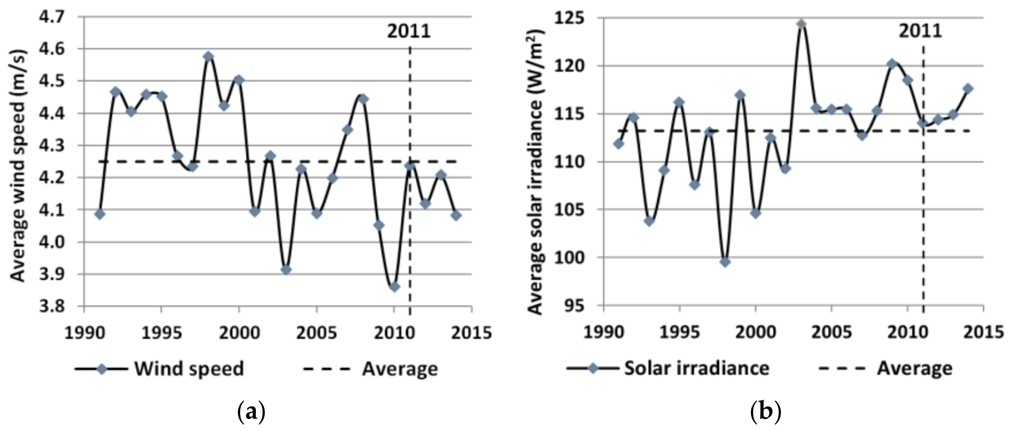
For determining the hourly electricity production of a selected wind turbine, first, the wind speed measured at ground level (
Figure A2a) is corrected to the wind speed at the hub height of the wind turbine (
Va), using a correction formula Equation (A1), which takes into account the measurement height (
Hm) at the weather station, the hub height of the wind turbine (
Ha), and the roughness of the measurement area (
Rm) (
Table A3 and
Table A4).
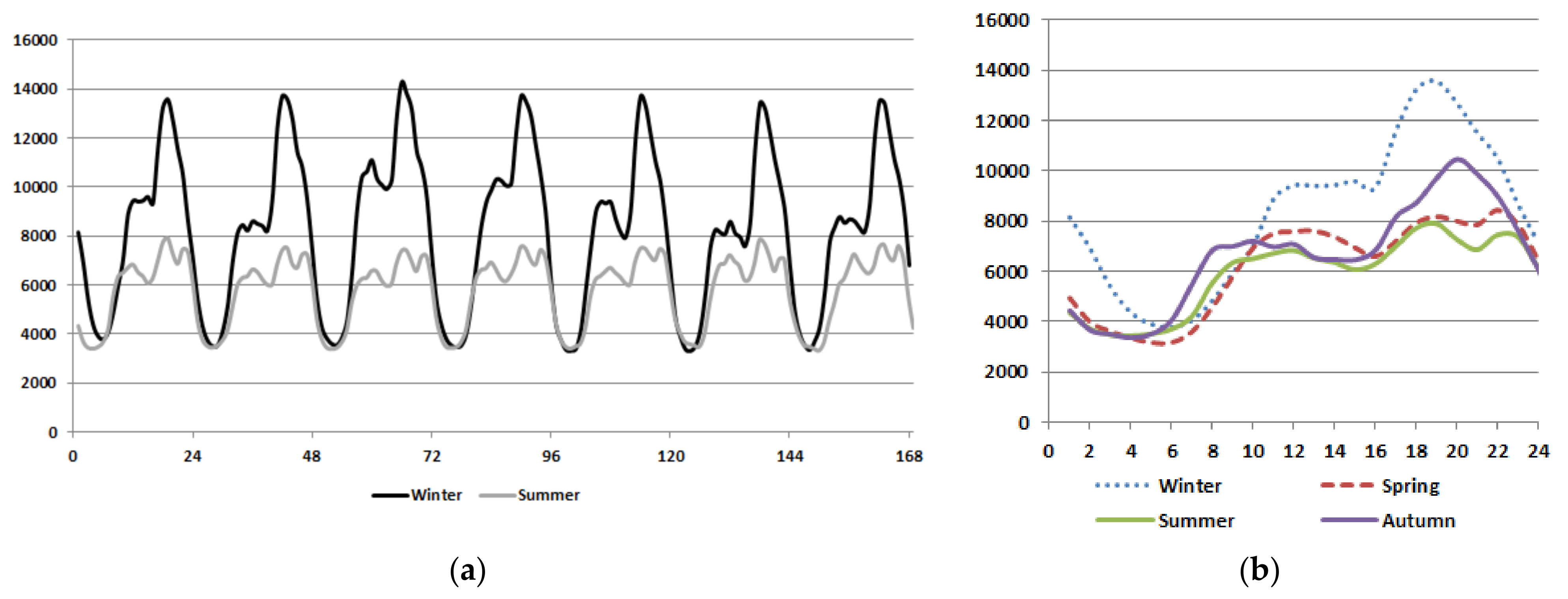
Figure A2.
(a) Wind speed adjusted for hub height, winter and summer week. (b) Solar irradiance ground, winter and summer week.
Figure A2.
(a) Wind speed adjusted for hub height, winter and summer week. (b) Solar irradiance ground, winter and summer week.
Table A5.
Values used for wind correction formula.
Table A5.
Values used for wind correction formula.
| | Unit | Measurement Site | Wind Turbine | Source |
|---|
| Height (Va) | m | 10 | 80 | [45,48] |
| Roughness length (Rm) | m | 0.055 | − | [69] |
Table A6.
Table used for determination of roughness class for wind speed correction calculation.
Table A6.
Table used for determination of roughness class for wind speed correction calculation.
| Landscape Description | Roughness Class
RC | Roughness Length
m | Energy Index
% |
|---|
| Water surface | 0 | 0.0002 | 100 |
| Completely open terrain with a smooth surface, such as concrete runways in airports, mowed grass | 0.5 | 0.0024 | 73 |
| Open agricultural area without fences and hedgerows within a distance of about 1250 m | 1 | 0.03 | 52 |
| Agricultural land with some houses and 8 m tall sheltering hedgerows within a distance of about 1250 m | 1.5 | 0.055 | 45 |
| Agricultural land with some houses and 8 m tall sheltering hedgerows within a distance of about 500 m | 2 | 0.1 | 39 |
| Agricultural land with many houses, scrubs, and plants or 8 m tall sheltering hedgerows within a distance of about 250 m | 2.5 | 0.2 | 31 |
| Municipality, small towns, agricultural land with many or tall sheltering hedgerows, forests, and very rough and uneven terrain | 3 | 0.04 | 24 |
| Larger cities with tall buildings | 3.5 | 0.8 | 18 |
| Very large cities with tall buildings and skyscrapers | 4 | 1.6 | 13 |
Second, the power of the wind turbine (
Pw) is determined using a set of conditions which include start up wind speed, ramp up, maximum production, and cut off wind speed, as shown in Equation (A2). The set of conditions are based on a 2 MW Vestas wind turbine [
48]. The ramp up production is determined through a polynomial trace line placed over the power curve of the selected wind turbine (
Figure A3).
Figure A3.
Power curve for on land Vestas V-80 2MW turbine [
48].
Figure A3.
Power curve for on land Vestas V-80 2MW turbine [
48].
Appendix D. Scenarios
The results indicted in this article are the culmination of multiple scenarios described in this appendix (
Figure A4).
Figure A4.
Scenarios used within this article.
Figure A4.
Scenarios used within this article.
The utilization of renewable technologies within the scenarios is based on merit order. The merit order determines which production technology has the right to produce first when multiple technologies are available. Within the scenarios, merit order is indicated by order of technology listed in the scenario name (
Figure A5).
Figure A5.
The principle of merit order in the scenario names.
Figure A5.
The principle of merit order in the scenario names.
- (2)
Renewable integration scenarios
Within the renewable integration scenarios (based on the renewable goals set by the EU for 2020, 2030, and 2050 [
65,
66]), a specific amount of intermittent RE production (a percentage of the total yearly electricity demand of the average municipality) will be placed in the municipality (
Table A7). The range of the scenarios will be between 0 and 100% I-RE in several steps to determine the effects on the balance indicators.
Table A7.
Installed capacity in kW of renewable resources in renewable integration scenarios.
Table A7.
Installed capacity in kW of renewable resources in renewable integration scenarios.
| Technology | REF | RE 20% | RE 60% | RE 100% | OptiMix | PV 100% | Wind 100% |
|---|
| Wind | 1411.7 | 3585.2 | 10,755.6 | 17,926.0 | 22,727.0 | 6,2753.0 | 0.0 |
| PV | 628.5 | 6275.3 | 18,825.9 | 31,377.0 | 22,973.0 | 0.0 | 35,852.0 |
- (3)
Renewable integration scenarios
These scenarios are used to indicate the effect of integrating intermittent renewable resources into the average municipality (
Table A8). The amount of renewable energy produced, of the total yearly demand of the average municipality, is indicated in the scenario name by the percentage of the total demand produced (e.g., “RE 60%”). The results from the scenarios will be compared to the REF scenario.
Table A8.
Renewable integration scenarios.
Table A8.
Renewable integration scenarios.
| Affiliation | Description of the Scenario |
|---|
| REF | 100% of the electricity will be retrieved from the national grid, including 4% wind and 1% solar PV electricity production [67]. |
| RE 20% | 20% of the total yearly demand of the average municipality will be produced by the intermittent RE sources of wind and solar PV, with a mix of 50% wind and 50% solar PV electricity production. |
| RE 60% | 60% of the total yearly demand of the average municipality will be produced by the intermittent RE sources of wind and solar PV, with a mix of 50% wind and 50% solar PV electricity production. |
| RE 100% | 100% of the total yearly demand of the average municipality will be produced by the intermittent RE sources of wind and solar PV, with a mix of 50% wind and 50% solar PV electricity production. |
| OptiMix 100% | 100% of the total yearly demand of the average municipality will be produced by the intermittent RE sources of wind and solar PV, with an optimum mix of wind and solar, looking at the lowest amount of overproduction. |
| PV 100% | In the RE 100% PV production scenario, 100% of the total yearly demand of the average municipality will be produced by the intermittent RE source of solar PV. |
| Wind 100% | In the RE 100% wind production scenario, 100% of the total yearly demand of the average municipality will be produced by the intermittent RE source of wind. |
Table A9.
Installed capacity in kW of renewable resources in renewable integration scenarios.
Table A9.
Installed capacity in kW of renewable resources in renewable integration scenarios.
| Technology | REF | RE 20% | RE 60% | RE 100% | OptiMix | PV 100% | Wind 100% |
|---|
| Wind | 1411.7 | 3585.2 | 10,755.6 | 17,926.0 | 22,727.0 | 62,753.0 | 0.0 |
| PV | 628.5 | 6275.3 | 18,825.9 | 31,377.0 | 22,973.0 | 0.0 | 35,852.0 |
| F-RE | − | − | − | − | − | − | − |
| ST | − | − | − | − | − | − | − |
| Grid | 14,405.7 | 14,405.7 | 14,405.7 | 14,405.7 | 14,405.7 | 14,405.7 | 14,405.7 |
Table A10.
Results from the renewable integration scenarios.
Table A10.
Results from the renewable integration scenarios.
| | REF | RE 20% | RE 60% | RE 100% | OptiMix | PV 100% | Wind 100% | Unit |
|---|
| Wind | 2377.0 | 6038.0 | 16,304.0 | 22,051.0 | 24,584.0 | 0.0 | 29,193.0 | MWh/a |
| PV | 605.0 | 6027.0 | 11,180.0 | 11,541.0 | 9364.0 | 23,662.0 | 0.0 | MWh/a |
| F-RE | 0.0 | 0.0 | 0.0 | 0.0 | 0.0 | 0.0 | 0.0 | MWh/a |
| ST | 0.0 | 0.0 | 0.0 | 0.0 | 0.0 | 0.0 | 0.0 | MWh/a |
| Grid | 57,399.0 | 48,316.0 | 32,896.0 | 26,789.0 | 26,433.0 | 36,719.0 | 31,188.0 | MWh/a |
| Surplus | 0.0 | 11.4 | 8743.8 | 26,788.5 | 26,433.0 | 36,718.9 | 31,187.9 | MWh/a |
| F-RE surplus | 0.0 | 0.0 | 0.0 | 0.0 | 0.0 | 0.0 | 0.0 | MWh/a |
| Peak production | 0.0 | 0.0 | 17,370.2 | 33,988.3 | 31,238.3 | 51,747.2 | 30,768.0 | kW |
| Peak demand | 14,252.6 | 14,241.8 | 14,206.4 | 14,171.0 | 14,147.3 | 14,405.7 | 14,082.5 | kW |
| Cost price | €0.20 | €0.20 | €0.20 | €0.21 | €0.21 | €0.21 | €0.21 | € |
| Grid expansion | €0.00 | €0.00 | €0.00 | €0.01 | €0.01 | €0.01 | €0.01 | € |
| F-RE | − | − | − | − | − | − | − | € |
| DSM | − | − | − | − | − | − | − | € |
| ST | − | − | − | − | − | − | − | € |
| Technology cost | − | − | − | − | − | − | − | € |
Figure A6.
Main yearly results from the renewable integration scenarios.
Figure A6.
Main yearly results from the renewable integration scenarios.
Figure A7.
Main LDC results from the renewable integration scenarios.
Figure A7.
Main LDC results from the renewable integration scenarios.
- (4)
Balancing technology scenarios
The following scenarios are used to indicate the effect of integrating balancing technologies resources into the average municipality. The RE production in the scenario is based on the OptiMix 100% scenario (
Table A11).
Table A11.
Local balancing technology scenarios.
Table A11.
Local balancing technology scenarios.
| Affiliation | Balancing Technology Scenarios |
| OptiMix | All the following scenarios will start with the installed capacity of the OptiMix scenario where 100% of the total yearly demand of the average municipality will be produced by the intermittent RE sources of wind and solar PV, with an optimum mix of wind and solar, looking at the lowest amount of overproduction. |
| +F-RE | In the (F-RE) scenario, an AD system will be installed (added to the OptiMix scenario), producing electricity for balancing purposes, operating an CHP unit at 120% capacity and calculating the BioAVE biomass availability (Table 4). |
| +DSM | In the DSM scenario, DSM will be installed in all households in the average municipality (added to the OptiMix scenario) utilizing the most common appliances in use today (Table 5). |
| +ST | In the ST scenario, the battery storage system will be based on the Tesla Powerwall (Table 6). For this scenario, 10% of the households will have a battery system (added to the OptiMix scenario). |
| Affiliation | Combined Balancing Technology Scenarios |
| +DSM + F-RE | In this scenario, DSM is combined with F-RE and added to the OptiMix scenario. The merit order, or order of deployment for the technologies, will be similar to the scenario name. |
| +F-RE + ST | In this scenario, F-RE is combined with ST and added to the OptiMix scenario. The merit order, or order of deployment for the technologies, will be similar to the scenario name. |
| +DSM + ST | In this scenario, DSM is combined with ST and added to the OptiMix scenario. The merit order, or order of deployment for the technologies, will be similar to the scenario name. |
| +DSM + F-RE + ST | In the combined scenario, multiple load balancing option is utilized (DSM, F-RE, and ST). The merit order, or order of deployment for the technologies, will be similar to the scenario name, where in DSM + ST, the merit order is first DSM and then ST. |
Table A12.
Installed capacity in kW of balancing technologies scenarios.
Table A12.
Installed capacity in kW of balancing technologies scenarios.
| Technology | F-RE | DSM | ST | DSM + F-RE | F-RE + ST | DSM + ST | DSM + F-RE + ST |
|---|
| Wind | 22,727.0 | 22,727.0 | 22,727.0 | 22,727.0 | 22,727.0 | 22,727.0 | 22,727.0 |
| PV | 22,973.0 | 22,973.0 | 22,973.0 | 22,973.0 | 22,973.0 | 22,973.0 | 22,973.0 |
| F-RE | 1150.1 | − | − | 1150.1 | 1150.1 | − | 1150.1 |
| ST | − | − | 13,858.0 | − | 13,858.0 | 13,858.0 | 13,858.0 |
| Grid | 14,405.7 | 14,405.7 | 14,405.7 | 14,405.7 | 14,405.7 | 14,405.7 | 14,405.7 |
Table A13.
Results from the balancing technologies scenarios.
Table A13.
Results from the balancing technologies scenarios.
| | F-RE | DSM | ST | DSM + F-RE | F-RE + ST | DSM + ST | DSM + F-RE + ST | Unit |
|---|
| Wind | 24,584.0 | 25,437.0 | 24,584.0 | 25,236.0 | 24,584.0 | 25,279.0 | 25,108.0 | MWh/a |
| PV | 9364.0 | 10,276.0 | 9364.0 | 10,059.0 | 9364.0 | 10,141.0 | 9952.0 | MWh/a |
| F-RE | 5851.0 | 0.0 | 0.0 | 6208.0 | 5851.0 | 0.0 | 6164.0 | MWh/a |
| ST | 0.0 | 0.0 | 6067.0 | 0.0 | 5698.0 | 5380.0 | 5068.0 | MWh/a |
| Grid | 20,583.0 | 24,668.0 | 20,366.0 | 18,877.0 | 14,885.0 | 19,582.0 | 14,089.0 | MWh/a |
| Surplus | 26,433.0 | 24667.8 | 18,879.3 | 25,084.8 | 19,241.1 | 18,211.6 | 18,851.9 | MWh/a |
| F-RE surplus | 2541.1 | 0.0 | 0.0 | 2184.4 | 2541.1 | 0.0 | 2229.1 | MWh/a |
| Peak production | 31,238.3 | 31,238.3 | 31,029.3 | 31,238.3 | 31,029.3 | 31,029.3 | 31,029.3 | kW |
| Peak demand | 12,997.2 | 14,147.3 | 14,147.3 | 12,997.2 | 12,997.2 | 14,147.3 | 12,997.2 | kW |
| Cost price | €0.21 | €0.23 | €0.23 | €0.23 | €0.23 | €0.25 | €0.25 | € |
| Grid expansion | €0.00635 | €0.01 | €0.01 | €0.01 | €0.01 | €0.01 | €0.01 | € |
| F-RE | €0.00000 | − | − | €0.00 | €0.00 | − | €0.00 | € |
| DSM | − | €0.02 | − | €0.02 | − | €0.02 | €0.02 | € |
| ST | − | − | €0.02 | − | €0.02 | €0.02 | €0.02 | € |
| Technology cost | €0.00 | €0.02 | €0.02 | €0.02 | €0.02 | €0.04 | €0.04 | € |
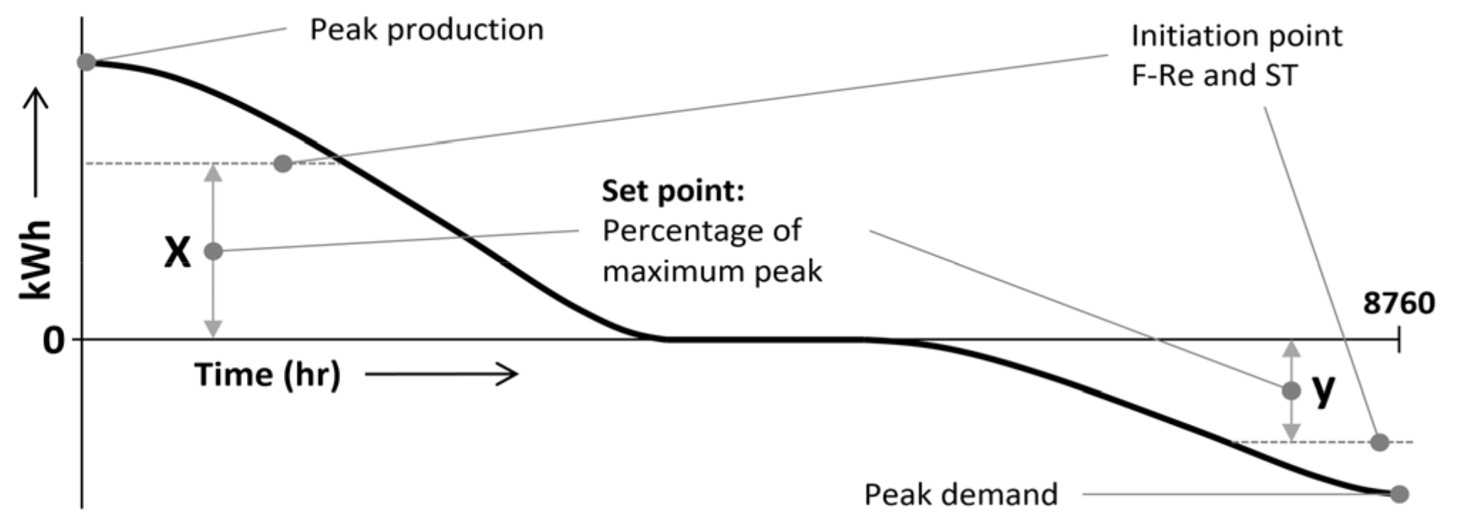
The following scenarios are used to indicate the effect of peak shaving on the maximum demand and production peak in the average municipality (
Table A14). A scenario using this option is indicated with “+Peak”, followed by the set point for peak production (
Figure A8, x) and the set point for peak demand (
Figure A8, y); both can be altered independently. For instance, if ST charges at 80% of the production peak and discharges at 0% of the demand peak (or the highest peak occurring in the average municipality) the scenario is indicated with “Peak 80–0%”, and if both set points are similar, “Peak 80%” is used.
Figure A8.
The principle of peak shaving in the PowerPlan model.
Figure A8.
The principle of peak shaving in the PowerPlan model.
Table A14.
Peak shaving scenarios.
Table A14.
Peak shaving scenarios.
| Affiliation | Description of the Scenario |
|---|
| OptiMix | All following scenarios will start with the installed capacity of the OptiMix scenario, where 100% of the total yearly demand of the average municipality will be produced by the intermittent RE sources of wind and solar PV, with an optimum mix of wind and solar, looking at the lowest amount of overproduction. |
| DSM + F-RE + ST + Peak 50% | In the +Peak scenarios, focus is placed on peak shaving using the peak shaving management described in applied to F-RE and ST. The range will be set from 50% to 80% of the maximum demand and production peak. |
| DSM + F-RE + ST + Peak 80% | In the +Peak scenarios, focus is placed on peak shaving using the peak shaving management described in applied to F-RE and ST. The range will be set from 50% to 80% of the maximum demand and production peak. |
| DSM + F-RE + ST + Peak 80–0% | In the +Peak scenarios, focus is placed on peak shaving using the peak shaving management described in applied to F-RE and ST. The range will be set from 50% to 80% of the maximum demand and production peak. |
Table A15.
Installed capacity in kW of peak scenarios.
Table A15.
Installed capacity in kW of peak scenarios.
| Technology | Peak 50% | Peak 80% | Peak 80–0% |
|---|
| Wind | 22,727.0 | 22,727.0 | 22,727.0 |
| PV | 22,973.0 | 22,973.0 | 22,973.0 |
| F-RE | 1150.1 | 1150.1 | 1150.1 |
| ST | 13,858.0 | 13,858.0 | 13,858.0 |
| Grid | 14,405.7 | 14,405.7 | 14,405.7 |
Table A16.
Results from the peak scenarios.
Table A16.
Results from the peak scenarios.
| | Peak 50% | Peak 80% | Peak 80–0% | Unit |
|---|
| Wind | 25,108.0 | 25,108.0 | 25,108.0 | MWh/a |
| PV | 9952.0 | 9952.0 | 9952.0 | MWh/a |
| F-RE | 2569.0 | 305.0 | 305.0 | MWh/a |
| ST | 1051.0 | 9.0 | 229.0 | MWh/a |
| Grid | 21,701.0 | 25,007.0 | 24,786.0 | MWh/a |
| Surplus | 23,293.0 | 25,069.5 | 23,314.2 | MWh/a |
| F-RE surplus | 5819.8 | 8079.3 | 8079.3 | MWh/a |
| Peak production | 31,029.3 | 31,029.3 | 31,029.3 | kW |
| Peak demand | 12,991.0 | 12,994.9 | 11,957.8 | kW |
| Cost price | €0.25 | €0.25 | €0.25 | € |
| Grid expansion | €0.01 | €0.01 | €0.01 | € |
| F-RE | €0.00 | €0.00 | €0.00 | € |
| DSM | €0.02 | €0.02 | €0.02 | € |
| ST | €0.02 | €0.02 | €0.02 | € |
| Technology cost | €0.04 | €0.04 | €0.04 | € |
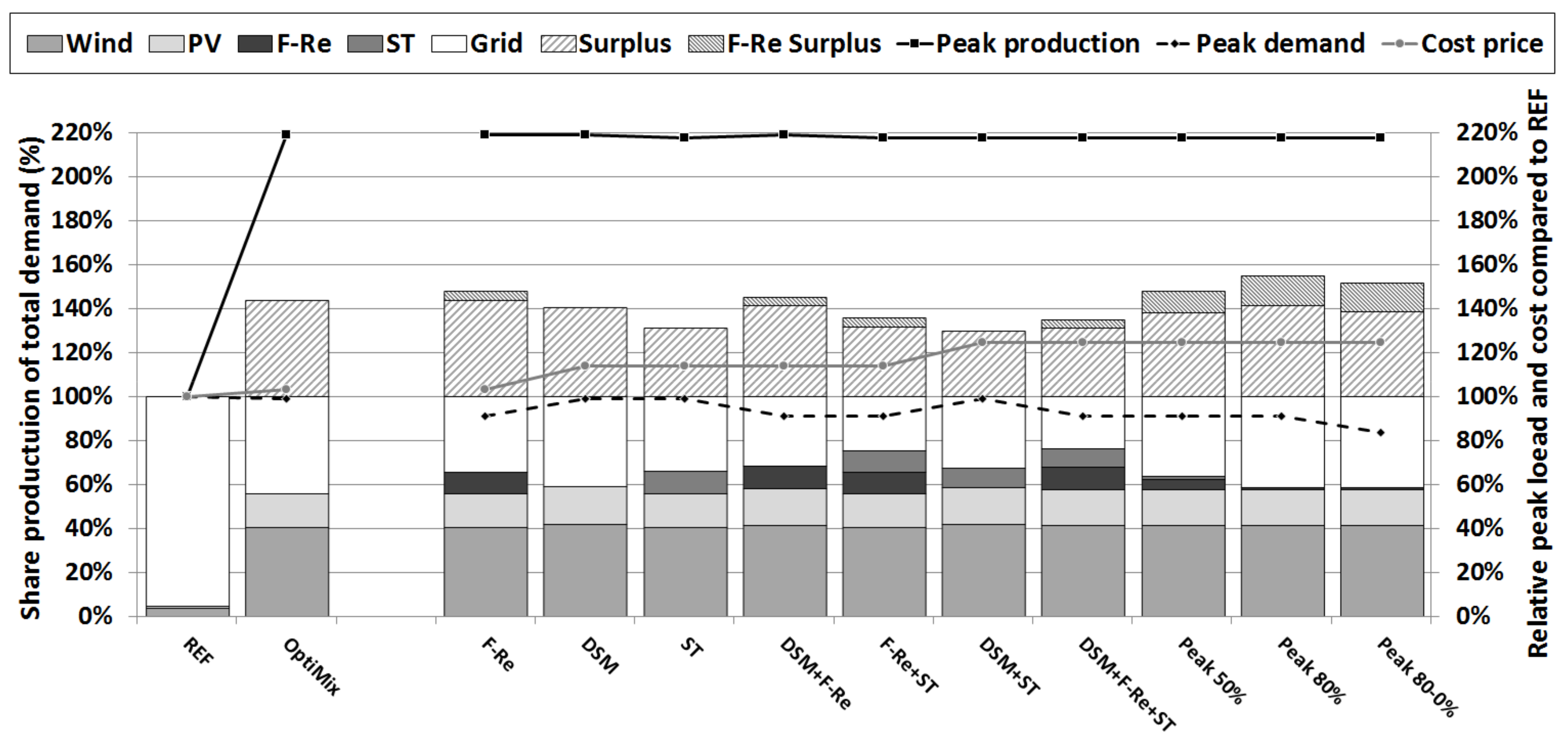
Figure A9.
Main yearly results from the renewable integration and peak shaving scenarios.
Figure A9.
Main yearly results from the renewable integration and peak shaving scenarios.
Figure A10.
Main LDC results from the renewable integration and peak shaving scenarios.
Figure A10.
Main LDC results from the renewable integration and peak shaving scenarios.
- (5)
Balancing technology scenarios
The following scenarios are used to indicate the effect of increasing the capacity of the balancing technologies and applying peak shaving to lower peak production and demand in the average municipality (
Table A17).
Table A17.
Increased capacity of balancing technology scenarios including peak shaving.
Table A17.
Increased capacity of balancing technology scenarios including peak shaving.
| Affiliation | Increased Capacity Scenarios |
| OptiMix | All the following scenarios will start with the installed capacity of the OptiMix scenario, where 100% of the total yearly demand of the average municipality will be produced by the intermittent RE sources of wind and solar PV, with an optimum mix of wind and solar, looking at the lowest amount of overproduction. |
| +DSM + F-RE + ST + Size 50% | In the +Size 50% scenario, the power rating of the CHP and the biogas storage size will be expanded with 500%. Battery storage size will be altered to 50% of the housing stock (Appendix C). |
| +DSM + F-RE + ST + Size 100% | In the +Size 100% scenario, the power rating of the CHP and the biogas storage size will be expanded with a 1000%. The battery storage size will be altered to 100% of the housing stock (Appendix C). |
| Affiliation | Increased Capacity Peak Shaving Scenarios |
| Size 100% | All following scenarios will start with the Size 100% scenario, where the power rating of the CHP and the biogas storage size will be expanded with a 1000%. Battery storage size will be altered to 100% of the housing stock (Appendix C). |
| +Peak 50% | In the +Peak 50% scenario, ST only charges above 50% of the production peak and ST and F-RE only discharge or operate above 50% of the demand peak. |
| +Peak 60% | In the +Peak 50% scenario, ST only charges above 60% of the production peak and ST and F-RE only discharge or operate above 60% of the demand peak. |
| +Peak 70% | In the +Peak 50% scenario, ST only charges above 70% of the production peak and ST and F-RE only discharge or operate above 70% of the demand peak. |
| +Peak 80% | In the +Peak 80% scenario, ST only charges above 50% of the production peak and ST and F-RE only discharge or operate above 80% of the demand peak. |
| +Peak 0–80% | In the +Peak 50% scenario, ST only charges above 0% of the production peak and ST and F-RE only discharge or operate above 80% of the demand peak. |
| +Peak 80–0% | In the +Peak 80% scenario, ST only charges above 50% of the production peak and ST and F-RE only discharge or operate above 0% of the demand peak. |
Table A18.
Installed capacity in kW capacity of balancing technology scenarios including peak shaving.
Table A18.
Installed capacity in kW capacity of balancing technology scenarios including peak shaving.
| Technology | Size 50% | Size 100% | Size 100% + Peak 50% | Size 100% + Peak 60% | Size 100% + Peak 70% | Size 100% + Peak 80% | Size 100% + Peak 0–80% | Size 100% + Peak 80–0% |
|---|
| Wind | 22,727.0 | 22,727.0 | 22,727.0 | 22,727.0 | 22,727.0 | 22,727.0 | 22,727.0 | 22,727.0 |
| PV | 22,973.0 | 22,973.0 | 22,973.0 | 22,973.0 | 22,973.0 | 22,973.0 | 22,973.0 | 22,973.0 |
| F-RE | 4792.2 | 9584.5 | 9584.5 | 9584.5 | 9584.5 | 9584.5 | 9584.5 | 9584.5 |
| ST | 69,289.1 | 138,578.2 | 138,578.2 | 138,578.2 | 138,578.2 | 138,578.2 | 138,578.2 | 138,578.2 |
| Grid | 14,405.7 | 14,405.7 | 14,405.7 | 14,405.7 | 14,405.7 | 14,405.7 | 14,405.7 | 14,405.7 |
Table A19.
Results from the balancing technology scenarios including peak shaving.
Table A19.
Results from the balancing technology scenarios including peak shaving.
| | Size 50% | Size 100% | Size 100% + Peak 50% | Size 100% + Peak 60% | Size 100% + Peak 70% | Size 100% + Peak 80% | Size 100% + Peak 0–80% | Size 100% + Peak 80–0% | Unit |
|---|
| Wind | 24,727.0 | 24,596.0 | 24,632.0 | 24,683.0 | 24,752.0 | 24,892.0 | 24,596.0 | 24,892.0 | MWh/a |
| PV | 9398.0 | 9364.0 | 9365.0 | 9372.0 | 9429.0 | 9673.0 | 9364.0 | 9673.0 | MWh/a |
| F-RE | 8418.0 | 8491.0 | 5031.0 | 2617.0 | 1141.0 | 384.0 | 8491.0 | 384.0 | MWh/a |
| ST | 7811.0 | 8513.0 | 1454.0 | 224.0 | 40.0 | 16.0 | 504.0 | 174.0 | MWh/a |
| Grid | 10,027.0 | 9417.0 | 19,899.0 | 23,484.0 | 25,019.0 | 25,416.0 | 17,426.0 | 25,258.0 | MWh/a |
| Surplus | 12,490.6 | 7333.6 | 16,172.4 | 21,360.6 | 23,711.6 | 24,688.7 | 25,291.3 | 10,731.0 | MWh/a |
| F-RE surplus | 26.4 | 0.0 | 3457.4 | 5708.7 | 7165.9 | 7916.6 | 0.0 | 7916.6 | MWh/a |
| Peak production | 30,193.1 | 29,147.8 | 29,147.8 | 29,147.8 | 29,147.8 | 27,541.1 | 27,541.1 | 29,147.8 | kW |
| Peak demand | 13,162.9 | 11,951.7 | 11,115.8 | 8643.2 | 10,084.0 | 14,086.0 | 12,266.9 | 11,524.4 | kW |
| Cost price | €0.32 | €0.43 | €0.43 | €0.43 | €0.43 | €0.43 | €0.43 | €0.43 | € |
| Grid expansion | €0.01 | €0.01 | €0.01 | €0.01 | €0.01 | €0.01 | €0.01 | €0.01 | € |
| F-RE | €0.00 | €0.01 | €0.01 | €0.01 | €0.01 | €0.01 | €0.01 | €0.01 | € |
| DSM | €0.02 | €0.02 | €0.02 | €0.02 | €0.02 | €0.02 | €0.02 | €0.02 | € |
| ST | €0.11 | €0.21 | €0.21 | €0.21 | €0.21 | €0.21 | €0.21 | €0.21 | € |
| Technology cost | €0.11 | €0.22 | €0.22 | €0.22 | €0.22 | €0.22 | €0.22 | €0.22 | € |
The following scenarios are used to indicate the effect of lowering RE production in the average municipality (
Table A20).
Table A20.
Lowering the RE production scenarios.
Table A20.
Lowering the RE production scenarios.
| Affiliation | Increased Capacity Scenarios |
|---|
OptiMix 60%
+ DSM + F-RE + ST + Size 50% | In this scenario, the RE production from the OptiMix scenario is lowered to 60% of the total yearly demand in the average municipality. DSM is installed in all the houses. The power rating of the CHP and the biogas storage size will be expanded by 500%. Battery storage size will be altered to 50% of the housing stock (Appendix C). |
OptiMix 60%
+ DSM + F-RE + ST + Size 100% | In this scenario, the RE production from the OptiMix scenario is lowered to 60% of the total yearly demand in the average municipality. DSM is installed in all the houses. The power rating of the CHP and the biogas storage size will be expanded by 1000%. Battery storage size will be altered to 100% of the housing stock (Appendix C). |
OptiMix 80%
+ DSM + F-RE + ST + Size 50% | In this scenario, the RE production from the OptiMix scenario is lowered to 80% of the total yearly demand in the average municipality. DSM is installed in all the houses. The power rating of the CHP and the biogas storage size will be expanded by 500%. Battery storage size will be altered to 50% of the housing stock (Appendix C). |
OptiMix 80%
+ DSM + F-RE + ST + Size 100% | In this scenario, the RE production from the OptiMix scenario is lowered to 80% of the total yearly demand in the average municipality. DSM is installed in all the houses. The power rating of the CHP and the biogas storage size will be expanded by 1000%. Battery storage size will be altered to 100% of the housing stock (Appendix C). |
Table A21.
Installed capacity in kW of the lowered RE production scenarios.
Table A21.
Installed capacity in kW of the lowered RE production scenarios.
| Technology | RE 60% + Size 50% | RE 60% + Size 100% | RE 80% + Size 50% | RE 80% + Size 100% |
|---|
| Wind | 13,636.2 | 13,636.2 | 18,181.6 | 18,181.6 |
| PV | 13,783.8 | 13,783.8 | 18,378.4 | 18,378.4 |
| F-RE | 4792.2 | 9584.5 | 4792.2 | 9584.5 |
| ST | 69,289.1 | 138,578.2 | 69,289.1 | 138,578.2 |
| Grid | 14,405.7 | 14,405.7 | 14,405.7 | 14,405.7 |
Table A22.
Results from the lowered RE production scenarios.
Table A22.
Results from the lowered RE production scenarios.
| | RE 60% + Size 50% | RE 60% + Size 100% | RE 80% + Size 50% | RE 80% + Size 100% | Unit |
|---|
| Wind | 18,989.0 | 18,989.0 | 22,210.0 | 22,210.0 | MWh/a |
| PV | 8768.0 | 8768.0 | 9239.0 | 9239.0 | MWh/a |
| F-RE | 8294.0 | 8492.0 | 7585.0 | 8078.0 | MWh/a |
| ST | 5641.0 | 5502.0 | 8784.0 | 9366.0 | MWh/a |
| Grid | 18,689.0 | 18,630.0 | 12,564.0 | 11,489.0 | MWh/a |
| Surplus | 682.7 | 114.2 | 4168.4 | 1322.2 | MWh/a |
| F-RE surplus | 150.1 | 0.0 | 842.6 | 346.6 | MWh/a |
| Peak production | 14,748.2 | 12,932.4 | 22,470.7 | 21,425.4 | kW |
| Peak demand | 13,242.0 | 13,035.1 | 13,217.4 | 12,971.5 | kW |
| Cost price | €0.31 | €0.42 | €0.32 | €0.43 | € |
| Grid expansion | €0.00 | €0.00 | €0.01 | €0.01 | € |
| F-RE | €0.00 | €0.01 | €0.00 | €0.01 | € |
| DSM | €0.02 | €0.02 | €0.02 | €0.02 | € |
| ST | €0.11 | €0.21 | €0.11 | €0.21 | € |
| Technology cost | €0.11 | €0.22 | €0.11 | €0.22 | € |
Figure A11.
Main yearly results from the lowered RE production scenarios.
Figure A11.
Main yearly results from the lowered RE production scenarios.
Figure A12.
Main LDC results from the lowered RE production scenarios.
Figure A12.
Main LDC results from the lowered RE production scenarios.
- (6)
Increased biomass potential scenarios combined with lowering RE production
The following scenarios are used to indicate the effect of increasing the biomass availability in the average municipality in combination with lowering RE production (
Table A23).
Table A23.
BioMAX scenarios.
Table A23.
BioMAX scenarios.
| Affiliation | Increased biomass potential scenarios |
| BioMAX | All following scenarios will start with the BioMAX scenario, which is based on a rural mainly agricultural municipality with high biomass availability (Table 4). |
| +OptiMix + F-RE | In the (F-RE) scenario, an AD system will be installed (added to the OptiMix scenario) producing electricity for balancing purposes, operating a CHP unit at 120% capacity. |
| +OptiMix + F-RE 500% | In the (F-RE) 500% scenario, an AD system will be installed (added to the OptiMix scenario) producing electricity for balancing purposes, operating a CHP unit at 500% capacity. |
| OptiMix + F-RE 1000% | In the (F-RE) 1000% scenario, an AD system will be installed (added to the OptiMix scenario) producing electricity for balancing purposes, operating a CHP unit at 1000%. |
| Affiliation | Increased biomass potential reduced RE production scenarios |
| +OptiMix 60% + DSM + F-RE 500% | In this scenario, the RE production from the OptiMix scenario is lowered to 60% of the total yearly demand in the average municipality. DSM is installed in all the houses. The power rating of the CHP and the biogas storage size will be expanded by 500%. |
| +OptiMix 60% + DSM + ST 50% + F-RE 500% | In this scenario, the RE production from the OptiMix scenario is lowered to 60% of the total yearly demand in the average municipality. DSM is installed in all the houses. The power rating of the CHP and the biogas storage size will be expanded by 500%. Battery storage size will be altered to 50% of the housing stock (Appendix C). |
| +OptiMix 60% + DSM + ST 100% + F-RE 500% | In this scenario, the RE production from the OptiMix scenario is lowered to 60% of the total yearly demand in the average municipality. DSM is installed in all the houses. The power rating of the CHP and the biogas storage size will be expanded by 500%. Battery storage size will be altered to 100% of the housing stock (Appendix C). |
| +OptiMix 60% + DSM + ST 50% + F-RE 1000% | In this scenario, the RE production from the OptiMix scenario is lowered to 60% of the total yearly demand in the average municipality. DSM is installed in all the houses. The power rating of the CHP and the biogas storage size will be expanded by 1000%. Battery storage size will be altered to 50% of the housing stock (Appendix C). |
Table A24.
Installed capacities in kW of the BioMAX scenarios.
Table A24.
Installed capacities in kW of the BioMAX scenarios.
| Technology | F-RE 120% | F-RE 500% | F-RE 1000% | RE 60% + DSM + F-RE 500% | RE 60% + DSM + ST 50% + F-RE 500% | RE 60% + DSM + ST 100% + F-RE 500% | RE 60% + DSM + ST 50% + F-RE 1000% |
|---|
| Wind | 22,727.0 | 22,727.0 | 22,727.0 | 13,636.2 | 13,636.2 | 13,636.2 | 13,636.2 |
| PV | 22,973.0 | 22,973.0 | 22,973.0 | 13,783.8 | 13,783.8 | 13,783.8 | 13,783.8 |
| F-RE | 4404.0 | 22,020.0 | 44,040.0 | 22,020.0 | 22,020.0 | 22,020.0 | 22,020.0 |
| ST | − | − | − | − | 69,289.1 | 138,578.2 | 69,289.1 |
| Grid | 14,405.7 | 14,405.7 | 14,405.7 | 14,405.7 | 14,405.7 | 14,405.7 | 14,405.7 |
Table A25.
Results from the BioMAX scenarios.
Table A25.
Results from the BioMAX scenarios.
| | F-RE 120% | F-RE 500% | F-RE 1000% | RE 60% + DSM + F-RE 500% | RE 60% + DSM + ST 50% + F-RE 500% | RE 60% + DSM + ST 100% + F-RE 500% | RE 60% + DSM + ST 50% + F-RE 1000% | Unit |
|---|
| Wind | 24,584.0 | 24,584.0 | 24,584.0 | 16,304.0 | 16,304.0 | 16,304.0 | 16,304.0 | MWh/a |
| PV | 9364.0 | 9364.0 | 9364.0 | 11,180.0 | 11,180.0 | 11,180.0 | 11,180.0 | MWh/a |
| F-RE | 8510.0 | 25,013.0 | 25,657.0 | 28,821.0 | 28,821.0 | 23,563.0 | 24,337.0 | MWh/a |
| ST | 0.0 | 0.0 | 0.0 | 0.0 | 451.0 | 6255.0 | 6255.0 | MWh/a |
| Grid | 17,923.0 | 1420.0 | 776.0 | 4076.0 | 3624.0 | 3078.0 | 2304.0 | MWh/a |
| Surplus | 26,433.0 | 26,433.0 | 26,433.0 | 8743.8 | 2610.7 | 329.4 | 329.4 | MWh/a |
| F-RE surplus | 0.0 | 7039.5 | 6175.2 | 3538.3 | 3538.3 | 8628.3 | 7986.8 | MWh/a |
| Peak production | 31,238.3 | 31,238.3 | 31,238.3 | 17,370.2 | 16,324.9 | 16,324.9 | 16,324.9 | kW |
| Peak demand | 13,206.9 | 9176.3 | 8439.6 | 9692.8 | 9528.5 | 9303.6 | 8439.6 | kW |
| Cost price | €0.21 | €0.22 | €0.23 | €0.24 | €0.34 | €0.45 | €0.35 | € |
| Grid expansion | €0.006 | €0.006 | €0.006 | €0.000 | €0.000 | €0.000 | €0.000 | € |
| F-RE | €0.008 | €0.013 | €0.023 | €0.013 | €0.013 | €0.013 | €0.023 | € |
| DSM | − | − | − | €0.022 | €0.022 | €0.022 | €0.022 | € |
| ST | − | − | − | − | €0.107 | €0.213 | €0.107 | € |
| Technology cost | €0.008 | €0.013 | €0.023 | €0.035 | €0.142 | €0.248 | €0.151 | € |
Figure A13.
Main yearly results from the BioMAX scenarios.
Figure A13.
Main yearly results from the BioMAX scenarios.
Figure A14.
Main LDC results from the BioMAX scenarios.
Figure A14.
Main LDC results from the BioMAX scenarios.


 ,
, 


