Electricity Consumption Forecast of High-Rise Office Buildings Based on the Long Short-Term Memory Method

Abstract

Various algorithms predominantly use data-driven methods for forecasting building electricity consumption. Among them, algorithms that use deep learning methods and, long and short-term memory (LSTM) have shown strong prediction accuracy in numerous fields. However, the LSTM algorithm still has certain limitations, e.g., the accuracy of forecasting the building air conditioning power consumption was not very high. To explore ways of improving the prediction accuracy, this study selects a high-rise office building in Shanghai to predict the air conditioning power consumption and lighting power consumption, respectively and discusses the influence of weather parameters and schedule parameters on the prediction accuracy. The results demonstrate that using the LSTM algorithm to accurately predict the electricity consumption of air conditioners is more challenging than predicting lighting electricity consumption. To improve the prediction accuracy of air conditioning power consumption, two parameters, relative humidity, and scheduling, must be added to the prediction model.

1. Introduction

As the basic industry of a national economy, the energy industry is not only an important guarantee for ensuring national strategic security but also a prerequisite for achieving sustainable economic development. Although China’s energy production and consumption are among the highest in the world, they have yet to be improved in terms of energy utilization efficiency, renewable energy development utilization rate, energy-saving, and emission reduction [1]. To cope with global climate change, energy-saving and emission reduction are crucial.

In recent years, many experts have investigated energy consumption to reduce energy and the environmental impact of urban building stocks. It has been suggested that predicting building energy consumption is an important step in solving various engineering problems. It not only enables us to understand and optimize the energy use of buildings but also explores potential energy-saving opportunities and proposes better strategies for sustainable urban development [2]. Building energy consumption prediction is the basic task of building energy management.

The optimization and management of energy consumption require a full understanding of building performance. The energy consumption of buildings and end-users, from various sources, should first be determined. Research on the end-use of building consumption shows that it can be grouped into heating, ventilation, and air conditioning systems (HVAC); lighting and plug-ins; special uses, including elevators, kitchen equipment, etc.; and auxiliary equipment and electrical appliances [3]. Among them, heating, ventilation, and air conditioning systems account for the majority of building energy consumption. Because the building energy prediction problem is a multivariate time prediction problem, accurately describing the energy consumption in a building is very complicated [4,5,6]. Conversely, energy consumption in a building depends upon many factors, such as weather conditions, thermal characteristics of the building envelope, occupancy behavior, and performance of the underlying components. However, the electricity consumed by buildings has obvious seasonal regularities and uncertainties [7].

At the same time, numerous approaches have been proposed. Some scholars have made a detailed summary of the existing prediction methods, such as Wei et al. [3] and Li et al. [8] Generally, the methods of predicting building electrical energy consumption are grouped into white box, gray box, and black-box methods [8]. The white box method is based on the physical parameters of the building and is modeled using modeling software for simulation. Currently, the three commonly used modeling software are DOE-2, EnergyPlus, and DeST [9]. DOE-2 is an early and widely used simulation software, and various simulation software have been derived as a computing core, such as eQuest, VisualDOE, EnergyPlus, etc. Energy Plus is a new generation of building energy efficiency simulation software, supported by the US Department of Energy. Currently, it is a core computing software without a graphical user interface. The software developed on its basis was DesignBuilder. DeST is a building energy simulation software, with AutoCAD as a graphical interface. The advantage of the white box method is that it does not require historical energy consumption data and can rely on the building’s physical parameters to predict the building’s energy consumption data. However, the disadvantage of the white box is that it cannot be calibrated using the actual historical data [8]. The gray box model refers to a statistical prediction method that combines the historical load information of a building with the physical information of the building [10]. The black box method is also called a data-driven method. It relies heavily on large amounts of historical building data. It uses strict mathematical derivation algorithms to predict data. Using the black box method is recommended when the historical data are sufficient and accurate, because its prediction accuracy is higher than that of the other two methods [3].

In recent years, many researchers have used data-driven black-box methods to predict the energy consumption of buildings. The data-driven method disregards the physics-based modeling process [11]. There are three main types of methods for using data-driven models to make time-series predictions, which are statistical analysis, machine learning, and deep learning. The autoregressive integrated moving average model (ARIMA) is the most common statistical analysis method. In recent years, some scholars have used ARIMA as a hybrid algorithm. De Nadai and Van Someren [12] combined the ARIMA model with an artificial neural network to predict natural gas consumption and achieve good performance. However, the ARIMA method relies heavily on historical data; if the data have great variability, they are not the right choice for predicting long-term time series [13]. Among the machine learning methods, K-nearest neighbors (KNN), artificial neural networks (ANNs), and support vector machines (SVMs) are more common for time series prediction. The core idea of the K-nearest neighbor algorithm is to predict the category of unlabeled samples, determined by the votes of the k nearest neighbors. However, each prediction of the K-nearest neighbor algorithm calculates the distance from the entire training set data to predict the data point, and then sorts the distances in increasing order, requiring significant calculation. Valgaev et al. [14] provided preliminary recommendations for a general short-term energy consumption forecasting model for buildings, based on the K-nearest neighbor method. The proposed model was automatically parameterized, generating predictions using only historical building load measurements as inputs. Artificial neural networks (ANNs) are effective nonlinear algorithms for time-series prediction [15]. Because they do not have linear characteristics and can fit any nonlinear function, they have become widely used algorithms. In addition, owing to the adaptive nature of artificial neural networks, artificial neural network models have become increasingly popular in prediction. Ferlit et al. [16] used the ANN algorithm to apply to real-world applications that included monthly historical building electricity consumption data sets. The SVM is a traditional prediction algorithm [17]. and is widely used in research because of its efficient model for solving nonlinear problems SVM can also be used to predict time series as it is effective in solving nonlinear regression estimation problems [18]. Dong et al. [19] first used SVMs to predict building energy consumption. This is the first application of an SVM for building load estimation research.

With the advent of cloud computing and big data, a significant increase in computing power can alleviate training inefficiencies and a large increase in training data can reduce the risk of overfitting, resulting in deep learning algorithms. A typical deep-learning model is a deep neural network. Compared with machine learning, deep learning not only increases the number of hidden layers but also the complexity of the system [20]. Among the commonly used deep learning algorithms, recurrent neural networks (RNNs) specifically deal with time-series problems. There are multiple time steps for the input of RNNs neurons and the input of each time step will share parameters when entering the neuron. Therefore, RNN can ‘memorize’ and ‘simulate’ the dependencies between data [21]. Long short-term memory (LSTM), as an RNN algorithm, is more complicated than RNN but addresses the problems of vanishing/exploding gradient. When there is a dependency relationship between data and a sequential relationship, the LSTM algorithm is generally considered first. Some scholars have used deep machine algorithms for building energy predictions. Fan et al. [22] confirmed that deep learning can improve the accuracy of building cooling load prediction, especially when using advanced functions as model inputs in an unsupervised manner. In their research, Wang et al. [20] compared thermal load predictions of the machine learning model XGBoost and the deep learning model LSTM. Wang believes that LSTM is only suitable for short-term load prediction and adding weather parameters helps to improve the robustness of LSTM.

However, few scholars currently use deep learning algorithms to predict the medium- and long-term energy consumption of buildings; it is difficult for the forecasting model to obtain more accurate results for the whole data set for long-term energy forecasting. On the other hand, the value of long-term energy consumption forecasting is less dependent on other parameters, while long-term forecasting appears more in regional energy consumption forecasting. Because the LSTM algorithm has a strong memory for time series, the annual energy consumption data may be reliably predicted using LSTM. This study attempts to use the LSTM algorithm to predict the energy consumption data for each day in the past two years by inputting hourly energy consumption data for each of these days.

To verify this idea, we collected air-conditioning energy consumption data for several office buildings in Shanghai and meteorological data from 2015 to 2017. The LSTM method was used to predict the air conditioning energy consumption of these office buildings in 2017. The final prediction results were compared with the actual building energy consumption of that year. The main contribution of this article lies in three aspects. First, unlike previous studies, air-conditioning and lighting electricity consumption data is based on hourly and sub-project measurements. Secondly, through LSTM model training, the data of the previous two years are used to predict the data of the next year. Such long-term forecasts did not exist in previous studies. Lastly, this work explores the influence of different parameters on improving the accuracy of the algorithm’s prediction. This study will help researchers use deep learning algorithms to further explore mid- to long-term energy consumption forecasting.

2. Data Analysis Methodology

There are still many difficulties in using the black box method to predict the electrical energy consumption of buildings. However, recently emerging deep-learning algorithms have attracted increased attention from many scholars. The well-known RNN algorithm in deep learning is widely used to predict time series [21] Many scholars have recently begun using LSTM to predict the electricity consumption of buildings. For example, Sendra-Arranz R [23] proposed several multistep prediction models based on LSTM neural networks. Zhou and Fang [24] used the deep learning long-term short-term memory (LSTM) model and Autoregressive Integrated Moving Average (ARIMA) and back-propagation (BP) network to predict the air-conditioning energy consumption of the Guangzhou University Library respectively. The results show that the LSTM model has reliable predictions. Wang and Du [13] proposed a novel approach based on an LSTM network for predicting periodic energy consumption. The results also proved that the prediction accuracy of LSTM is better than ARIMA and BP. This article will also start with the LSTM method to discuss the electricity consumption forecast of office buildings.

2.1. Research Route

This section describes the main work in this study.

The first step was a cognitive project. Having a correct understanding of the research object is the first and most important step in this research; thus, an on-site inspection of the office building was conducted to record and obtain the energy consumption and other relevant information of the building.

The second step was data preparation to ensure the accuracy of the data information; preliminary check of the data distribution map to ensure that the electricity consumption data is valid, i.e., there should be no zero or negative values, and there should be no extreme values outside the range. For continuous periods of electricity consumption, cases in which the value remains constant should also be eliminated. However, the content of the data should be as rich as possible for subsequent data screening.

The third step was data processing. After data collection, the first step is to collate and process the data. There are very few detailed and complete building information materials in the data obtained from field investigations. Among the obtained data, there are many invalid data or abnormal data, which require data washing. The types of data that need to be cleaned include the electricity consumption data of non-high-rise office buildings, abnormal energy consumption data, NA values in the original data, and discrete values.

The fourth step was the model prediction. LSTM was used to construct the building prediction model. Weather, building information, and building historical power consumption were selected as the input layer of the model and the estimated power consumption of the building was selected as the output layer. Then machine learning was used to build the prediction model of the building. From the data, 17,520 h of building electricity data from the first two years were used for model training, and 8760 h of building electricity data from the last year were used for model testing. Random sampling was not used for cross-validation, based on the temporal characteristics of LSTM.

The fifth step was model evaluation, i.e., analyzing and comparing the electricity consumption predicted by the model with the actual electricity consumption of the building. If there is a large difference between the predicted and real data, the process is repeated from the fourth step to rebuild the model and filter out invalid indicators or add new indicators.

2.2. Data Description

The data in this study were obtained from the actual building data of an office building in Shanghai. The office building has 30 floors above ground and 4 floors underground, with a total construction area of 101,806 m². The air conditioner used a full-air variable air volume system. In this study, LSTM can predict changes in the building through the most basic data and thus, other information from the site survey, such as building envelopes and air conditioning equipment information, has not been applied. The air-conditioning system of the office building adopted centralized cooling. There are two chillers in an AC system. The COP of the two units was 5.6 and the cooling capacities were 1758 kWh and 2813 kWh, respectively. The electricity consumption of the building’s air conditioning, lighting, and sockets was collected every hour.

At present, when some scholars use LSTM for building energy consumption prediction, they only use the historical data of the building to verify the accuracy of LSTM prediction and use the data from the previous day to predict the current day’s data. However, these historical load data cannot be used alone as a training indicator. The weather is still the primary influence on the energy consumption of building air conditioning [25]. Therefore, this study obtained weather data from the Shanghai Hongkou Weather Station.

Shanghai has a subtropical monsoon climate zone. There are four different seasons throughout the year, with plenty of sunshine and abundant rainfall. In 2016, the average temperature in Shanghai was 18.28 °C, and the average relative humidity was 73%.

2.3. Data Processing

2.3.1. Data Cleaning

The obtained data cannot be directly used for model training and must be processed first, that is, data cleaning. The purpose of data cleaning is to find and correct identifiable errors in the data files. The main process includes handling invalid and missing values and checking data consistency. First, we deleted any unavailable data. For some NA data in the dataset, the method used in this modeling is to delete all of these data instead of using a variable average or median. Second, abnormal data was cleared to avoid abnormal phenomena such as negative numbers or large data volumes. Finally, this study uses a method based on violin illustration detection to filter the data and eliminate outliers. The variables to be filtered include dry bulb temperature (Ta), dew point temperature (Td), relative humidity (RH), pressure (P), and wind speed (WS). Figure 1 shows the violin distributions of the above five variables. The average dry bulb temperature is approximately 19 °C, the average wet bulb temperature is approximately 13 °C, and the average relative humidity is 72%.

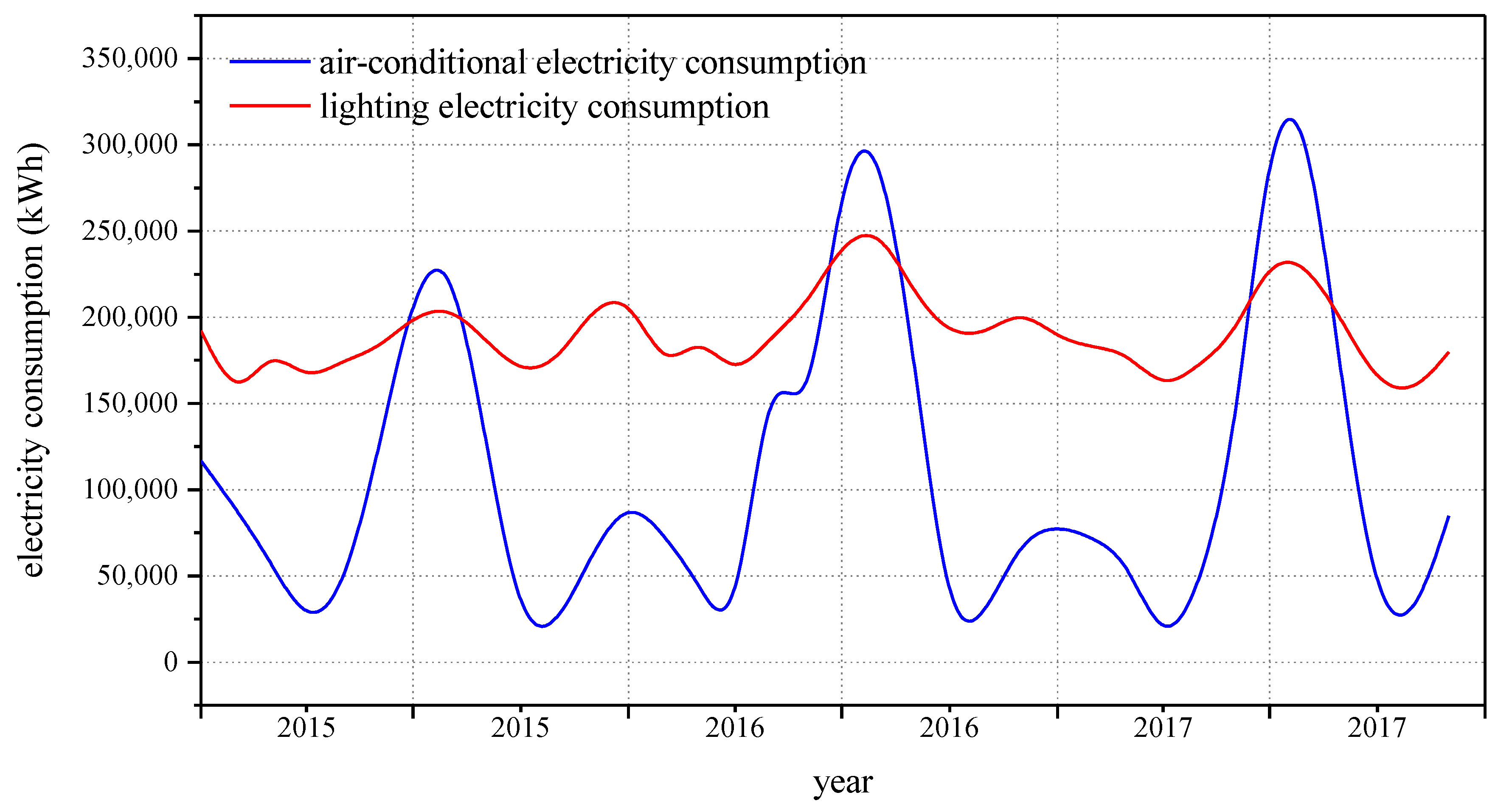
2.3.2. Data Analysis

After data filtering, the basic electricity consumption of the office building can be visually analyzed first, as shown in Figure 2 below, which shows the total monthly electricity consumption of the office building from 2015 to 2017. The blue curve represents the air conditioning energy consumption, and the red line represents the lighting and Socket energy consumption.

As shown in Figure 2, the electricity consumption of this office building has an obvious law, that is, the annual fluctuations of electricity consumption are similar. The power consumption of the air conditioner represented by the blue curve fluctuates greatly. It consumes more power in winter and summer, and less power in spring and autumn. The air-conditioning power consumption in the highest month exceeds the lighting power consumption. The total power consumption of lighting and sockets represented by the red curve is higher than the power consumption of air conditioners, but it does not change much between seasons. The highest power consumption also occurs during summer. On the other hand, it can be seen from Figure 2 that over time, the air-conditioning power consumption of office buildings in peak months has gradually increased over time, while the power consumption of lighting and sockets has no obvious annual change trend.

2.3.3. Correlation Analysis

Correlation analysis was used to identify the correlations between different variables. By identifying highly interdependent variables, the number of variables input to the model can be reduced to simplify the model. The range of the correlation coefficient (COR) was −1 to 1, indicating the degree of correlation between the variables. COR = 0 indicates that there is no relationship between the two variables. COR = 1 indicates a completely positive correlation and COR = −1 indicates a fully negative correlation. There are currently two types of correlation analysis that are used more frequently, i.e., Pearson correlation analysis and Spearman correlation analysis.

The Pearson correlation coefficient (PCC) is suitable for continuous data and requires that the data population is normally distributed or close to a normal unimodal distribution [26]. The Spearman correlation coefficient (SCC) [27], does not require the distribution of the original variables and is a non-parametric statistical method. It is mainly used to measure the degree of correlation between hierarchical ordinal variables, but its statistical power is lower than Pearson’s correlation coefficient. Considering that the Schedule parameters used in this study were ordinal—not continuous—variables and electricity consumption data were non-normally distributed the Spearman correlation coefficient was used to calculate the correlation when performing correlation analysis. The electricity data distribution diagram is shown in Figure 3.

2.4. LSTM Algorithm

Long Short-Term Memory (LSTM) is a recursive neural network. Its appearance solves the problems of gradient disappearance and gradient explosion in long-sequence training. Compared with traditional recurrent neural networks, long-term and short-term memory increase the connection between data [28].

The main input and output differences between the LSTM structure (right in the figure) and the ordinary RNN are shown in Figure 4.

Compared with RNN, which only has one transfer state $h^t$, LSTM has two transmission states, one $c^t$ (cell state) and one $h^t$ (hidden state). Among them, $c^t$ changes very slowly. Usually, the output $c^t$ is $c^{t-1}$, transmitted from the previous state with some values. However, $h^t$ is often very different for different nodes.

The internal structure of the LSTM is analyzed below. First, the current input of $x^t$ of LSTM and $h^{t-1}$ is passed down from the previous state to obtain four states.

$$\begin{gathered} z=\tanh (w_z{x}_t+U_z{h}_{t-1}+b_z) \\ {z}_f=\sigma (w_f{x}_t+U_f{h}_{t-1}+b_f) \\ {z}_i=\sigma (w_i{x}_t+U_i{h}_{t-1}+b_i) \\ {z}_o=\sigma (w_o{x}_t+U_o{h}_{t-1}+b_o) \end{gathered}$$

(1)

$z^{}$, $z_f$, $z_i$, and $z_o$ are all calculated by multiplying the input variable matrix by the weight matrix and adding the deviation; $z^{}$ converts the result to a value between −1 and 1 through a tan activation function, while $z_f$, $z_i$, and $z_o$ convert it to a value between 0 and 1 through the activation function of the gated state.

$z_f$, $z_i$, and $z_o$ relate to the input gate, forget gate, and output gate, respectfully. $w_z$, $w_i$, $w_f$, $w_o$, $U_z$, $U_i$, $U_f$, and $U_o$ are weight matrices. $b_z$, $b_f$, $b_i$, and $b_o$ are the bias vectors. $x_t$ is the current input, $h_{t-1}$ is the hidden layer output of the previous node.

$\tanh$ is used to convert the result into a value between −1 and 1 through a hyperbolic tangent activation function. The $sigmoid$ function and tanh function are defined as:

$$\begin{gathered} \sigma (x)=\frac{1}{1+e^{-x}} \\ \tanh (x)=\frac{e^x-e^{-x}}{e^x+e^{-x}} \end{gathered}$$

(2)

The following starts to further introduce the use of these four states in LSTM. Figure 5 shows the LSTM algorithm structure.

There are three main stages within LSTM:

(1)

‘Forget’ stage. Here, the input of the previous node is selectively ‘forgotten’. This stage controls the information from the previous state that needs to be retained and the previous state that needs to be forgotten.

$$\begin{gathered} z_f=\sigma (w_f{x}_t+U_f{h}_{t-1}+b_f) \\ {k}_t=c_{t-1}\odot z_f\left(\mathrm{forget}\mathrm{stage}\right) \end{gathered}$$

(3)

(2)

‘Storage’ stage. Here, the inputs of this stage are selectively ‘remembered’. Based on the results of previous calculations, this stage selectively stores and inputs the current amount of information.

$$\begin{gathered} z_i=\sigma (w_i{x}_t+U_i{h}_{t-1}+b_i) \\ z=\tanh (w_z{x}_t+U_z{h}_{t-1}+b_z) \\ {j}_t=z_i\odot z\left(\mathrm{storage}\mathrm{stage}\right) \\ {c}_t=j_t+k_t \end{gathered}$$

(4)

(3)

‘Output’ stage. This stage determines the output of the current state. At this stage, the results obtained in the previous stage are scaled (changed by the tanh activation function) and the amount of current information flowing into the subsequent network is controlled. The results obtained in the first and second steps for transmission are added to the next network. This is the first formula shown in the figure above.

$$\begin{gathered} z_o=\sigma (w_o{x}_t+U_o{h}_{t-1}+b_o) \\ {h}_t=\tanh (c_t)\odot z_o\left(\mathrm{output}\mathrm{stage}\right) \\ {y}_t=\sigma (W^{’}{h}^t) \end{gathered}$$

(5)

3. Results

In this section, the LSTM method is used to predict the power consumption of an office building in Shanghai. The significance of this study is not only to use LSTM to predict the energy consumption of buildings but also to explore the models and methods that affect the prediction accuracy by using LSTM methods. Previous scholars only used the LSTM method to conduct preliminary exploration and verification of the total load forecast for buildings, but no scholars have tried to use this method to separately predict the air-conditioning load and lighting load. Therefore, the results of this study further propose ways to improve the prediction accuracy of the LSTM method.

In the LSTM prediction process, the core variable is electricity consumption, and historical electricity consumption can be used as the only input variable to achieve a certain degree of accuracy. To explore whether adding other variables can change the prediction accuracy, the other variables will be added to study how the addition of these variables will affect prediction accuracy and these variables will be adjusted to improve the prediction accuracy.

3.1. Correlation Analysis of Auxiliary Variables

3.1.1. Correlation Analysis

Because electricity consumption data are not normally distributed, the Spearman correlation coefficient is used to express the correlation between auxiliary parameters and electricity consumption data. These auxiliary variables include dry-bulb and wet-bulb temperatures, relative humidity, pressure, and schedule parameters. The results of the correlation analysis are presented in

Table 1. The correlation between the auxiliary parameters and the power consumption data.

Correlation Coefficient	Electricity Consumption	Humidity	Dry-Bulb Temperature	Wet-Bulb Temperature	Pressure	Schedule Parameter
electricity consumption	1.000
humidity	−0.301	1.000
dry-bulb temperature	0.171	−0.040	1.000
wet-bulb temperature	0.074	0.355	0.900	1.000
pressure	−0.059	−0.223	−0.855	−0.876	1.000
schedule parameter	0.365	−0.008	−0.006	−0.004	−0.004	1.000

.

Table 1 summarizes these three key points. First, the correlation between air conditioning energy consumption data and other auxiliary parameters is not very high, and the three auxiliary variables with a higher correlation with load data are the schedule parameters, relative humidity, and dry bulb temperature. Second, among the input variables, the correlation among the schedule parameters, relative humidity, and dry bulb temperature was very low, demonstrating that these three variables have a low correlation. Finally, there was a strong correlation between dry bulb temperature, wet bulb temperature, and atmospheric pressure. The absolute value of the correlation coefficient between these variables exceeds 0.8, indicating that these three parameters are interchangeable. Based on the above analysis, we finally discarded the two parameters—wet bulb temperature and atmospheric pressure—and selected dry bulb temperature, schedule parameters, and relative humidity as auxiliary variables.

3.1.2. Meteorological Parameters

As mentioned in the Methods section, meteorological parameters have always been a factor that cannot be ignored in building energy consumption forecasting. It is a natural idea to include meteorological parameters in LSTM forecasting. Through data collection, we collected hourly meteorological data from the Shanghai Hongkou Weather Station from 2015 to 2017, including dry bulb temperature, wet bulb temperature, relative humidity, atmospheric pressure, and wind speed. Through correlation analysis, we found a clear correlation between dry bulb temperature, wet bulb temperature, and atmospheric pressure. Therefore, the two meteorological parameters—wet bulb temperature and atmospheric pressure—were deleted. Because wind speed, a meteorological parameter, affects air conditioning consumption in buildings with natural ventilation—but has little effect on the electricity consumption of high-rise buildings (especially office buildings) [29]—wind speed is not considered here. The remaining dry-bulb temperature and relative humidity were selected as variables among the meteorological parameters.

3.1.3. Schedule Parameters

To determine whether to use electrical appliances as a determinant of electricity consumption, it is necessary to consider when the office building uses more/less electricity [10]. For office buildings, electricity consumption is very regular. For the energy consumption of buildings, office buildings use more electricity during the day and less electricity at night. There is an obvious time dependency; therefore LSTM, an algorithm that specifically deals with timing issues, is very suitable for predicting energy consumption in office buildings. However, it is not sufficient to pay attention to the electricity consumption time. Most office buildings are closed during national legal holidays, such as the Spring Festival or National Day. During the holiday season, the building’s electricity consumption level is even lower than at night on weekdays. During national legal holidays, such as the Spring Festival, the time is not fixed, so it is necessary to add a variable ‘schedule’ to constrain the prediction model.

3.2. Model Description

The results of this experiment are divided into an air-conditioning electricity consumption forecast and a lighting electricity consumption forecast. According to the LSTM method, the parameters used in the input layer and the result of the output layer need to be set. In this study, the historical electricity consumption of the building as the output variable, and other relevant parameters were used as the input variable, and the LSTM network model was first established through the model training set. Then, the pertinent parameters of the test group were verified in the model and the power consumption of the building was predicted to verify the accuracy of the model. In accordance with previous studies [30], 50 neurons were set in the hidden layers in the LSTM model, 1 neuron was set in the output layer (regression problem), the input variable was a characteristic of the time step (t-n), the loss function used the ‘mean_squared_error’, the ‘Adam Optimizer’ was used as an optimization algorithm, the model used 200 epochs, and the size of each batch was 72.

The accuracy of the energy consumption forecast results can be evaluated by using indicators such as the mean square error (MSE), mean absolute error (MAE), and coefficient of variation of the root mean square error (CV-RMSE) [31].

$$\begin{gathered} \mathrm{MSE}=\frac{{\displaystyle \sum _{k=1}^n{\left(Y(k)-Y_p(k)\right)}^2}}{n} \\ \mathrm{MAE}=\frac{1}{n}{\displaystyle \sum _{k=1}^n\left|Y(k)-Y_p(k)\right|} \\ \mathrm{CV}-\mathrm{RMSE}=\frac{\sqrt{\frac{{\displaystyle \sum _{k=1}^n{\left(Y(k)-Y_p(k)\right)}^2}}{n}}}{\overline{Y}} \end{gathered}$$

(6)

where $Y(k)$ and $Y_p(k)$ are the actual and the predicted values, respectively, and $\overline{Y}$ denotes the average values.

MSE can accurately reflect the precision of the prediction results, MAE can measure its accuracy and CV-RMSE is the percentage of the root-mean-square error and the actual average value, reflecting the degree that the forecast value deviates from the actual value. The proposed model was established on an ordinary computer with Intel Core i5 and 16 GB of memory while the platform was Python 3.6. The packages used in Python include: numpy, pandas, sklearn, and keras.

3.3. Forecast Results Analysis

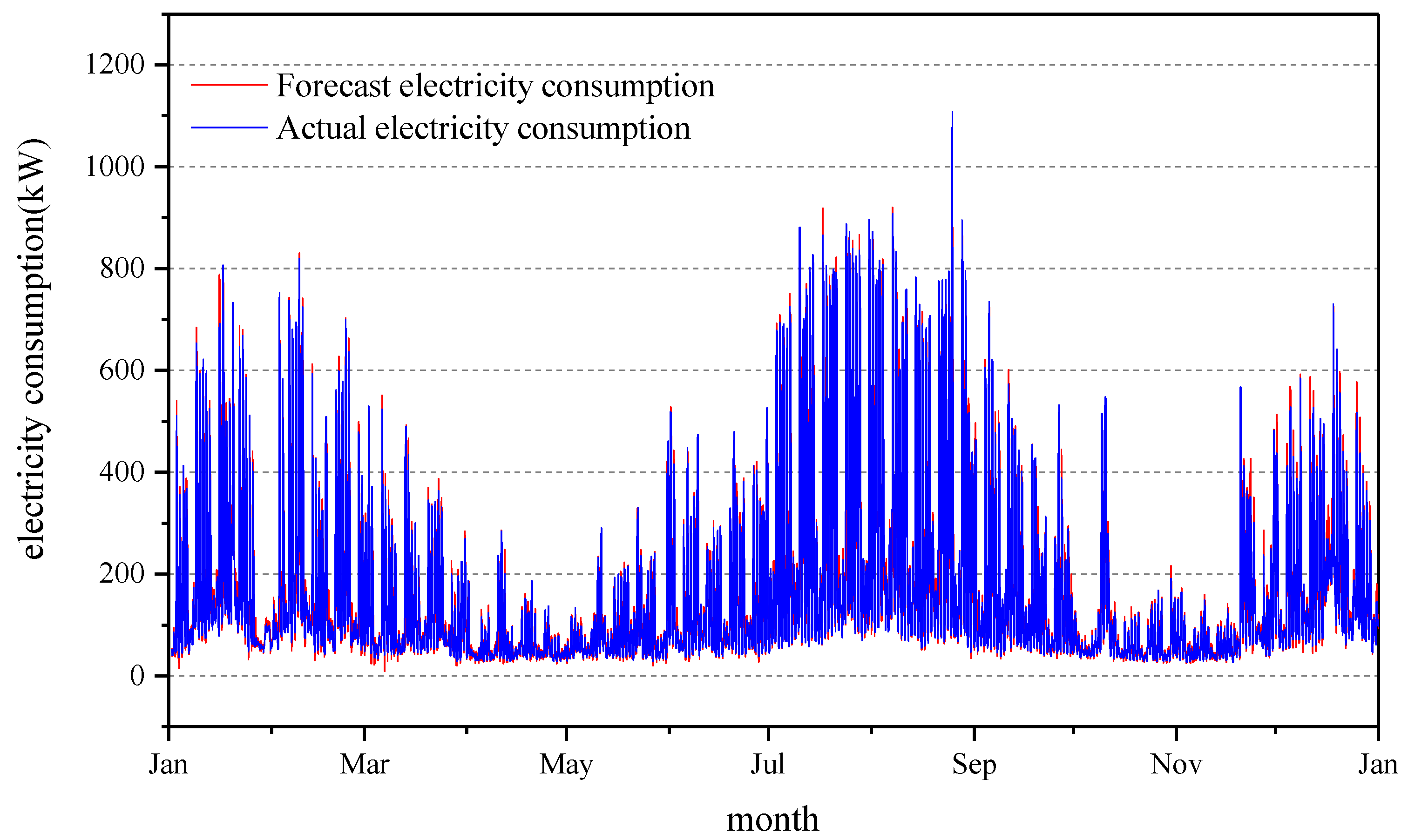
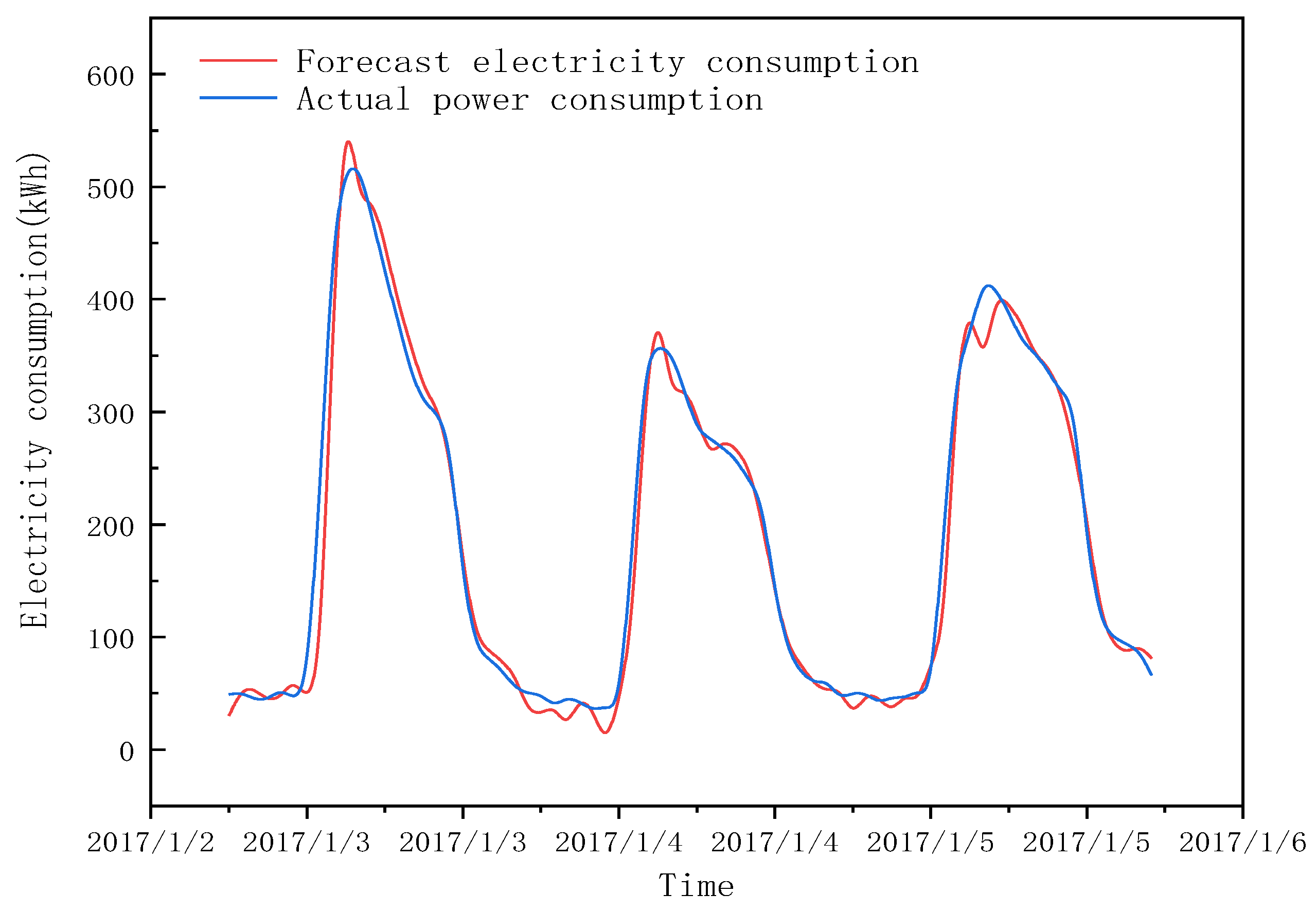
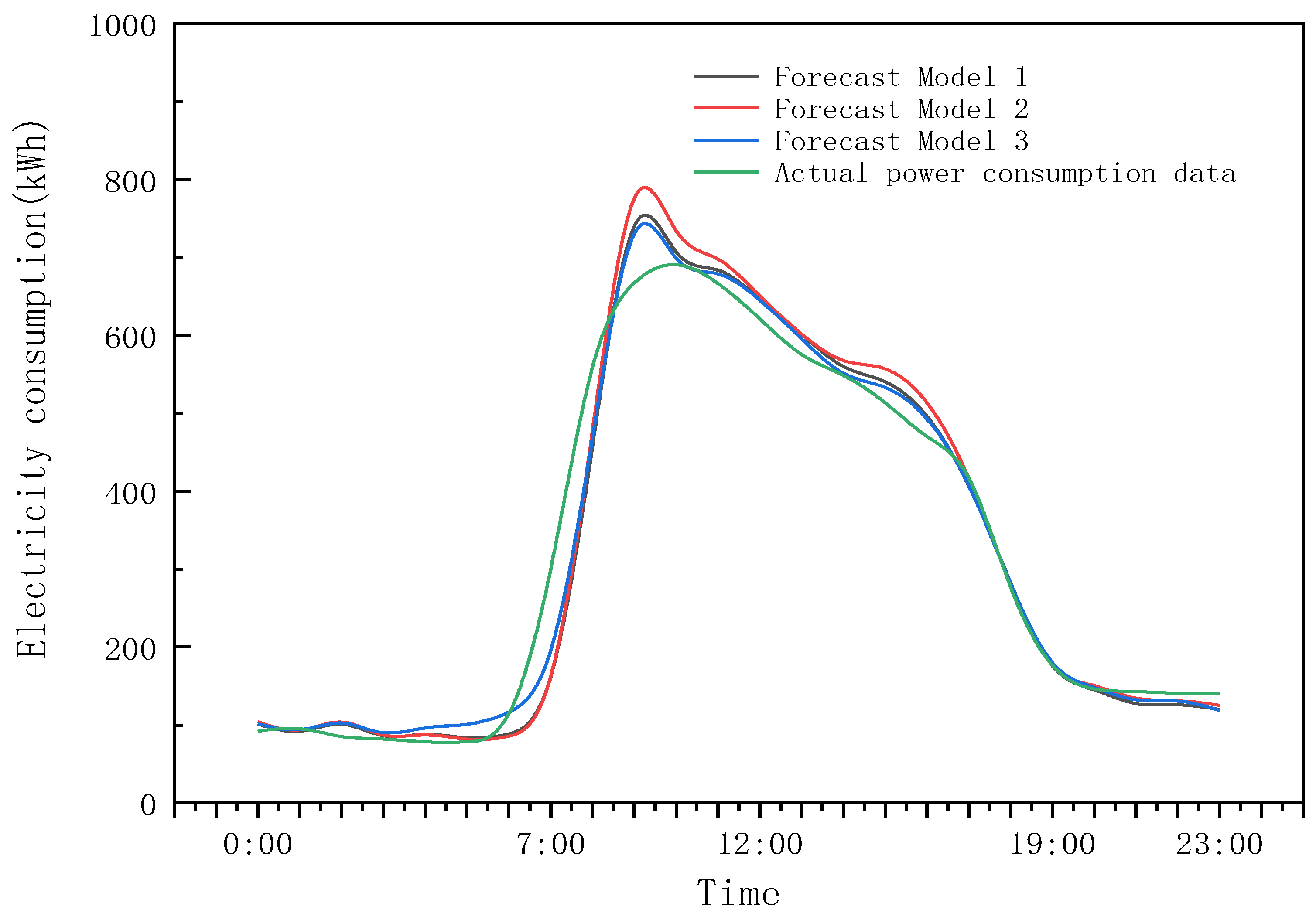
3.3.1. Model Comparison of Hourly Energy Consumption Prediction

For the black-box-based prediction model, various methods must be applied and then compared, and thus we introduced the ARIMA algorithm and BP algorithm as benchmarks for validating the performance of the LSTM algorithm used in this case. ARIMA and BP are considered as the widely used methods with good capabilities. The main principle of ARIMA is to first transform the non-stationary time-series data into the stationary time-series data, and then use the historical data of the variables to predict themselves [12]. The following formula shows the basic principles of the model.

$$\begin{array}{lll}{f}_t(p,d,q)& =& (1+{\phi }_1)f_{t-1}+({\phi }_2-{\phi }_1)f_{t-2}+\cdots +({\phi }_p-{\phi }_{p-1})f_{t-p}\\ & & -{\phi }_p{f}_{t-p-1}+e_t-{\theta }_1{e}_{t-1}-\cdots -{\theta }_2{e}_{t-2}-\cdots -{\theta }_q{e}_{t-q}\end{array}$$

(7)

where $t$ is the number of days, $p$ is the lag of the time series data, $d$ is the differential order of the time series data that needs to be stable, and $q$ is the lag of error used in forecast model.

The BP algorithm, a basic neural network, is able to implement the prediction but cannot remember the historical data [24], which may not be suitable for dealing with the time series forecasting problems. The setting of the BP neural network was that the electricity consumption data of the first 24 h was used as the data input layer, and the electricity consumption data of the next hour was used as the output layer.

The air-conditioning power consumption prediction was used for comparison among the BP, ARIMA, and LSTM methods. All the methods selected the hourly power consumption data of air conditioners from 2015 to 2016 as the training set and the hourly power consumption data of air conditioners in 2017 as the test set, respectively. To better illustrate the pros and cons of the three methods, we showed the daily electricity consumption forecast results for a week in 2017. The test set prediction results are shown in Figure 6.

As shown in Figure 6, it is obvious that LSTM has a better performance than ARIMA during weekdays, and the BP’s prediction results are the worst. The error between the daily prediction results of LSTM and the real data is no greater than 20 kWh. At the same time, we also calculated the MSE, MAE, and CV-RMSE for the three methods. The results are shown in

Table 2. Results of different models forecasting daily air-conditional electricity consumption.

Evaluation Index	MSE	MAE	CV-RMSE
LSTM	618.40	15.34	0.147
ARIMA	650.51	21.73	0.183
BP	721.36	35.32	0.276

. Compared with the ARIMA and BP, LSTM has a lower value in MSE, MAE, and CV-RMSE. The results showed that the LSTM model is superior to the ARIMA and BP neural network models in air conditioning energy consumption prediction. Therefore, using the LSTM method to train the hourly power consumption data of the first two years to predict the power consumption of the office building in the next year, has a better prediction accuracy than the other two algorithms.

3.3.2. Air-Conditioning Electricity Consumption Forecast

Figure 7 shows the air-conditioning electricity consumption forecasting graph in which only historical data are input. The blue line represents the actual power consumption of the air conditioner in the office building, and the red line represents the power consumption predicted by the LSTM. It can be seen from Figure 8 that the prediction is relatively accurate when the model only uses historical energy consumption data as input variables.

Figure 8 and Figure 9 show the winter air conditioning forecast and summer forecast, respectively. These two prediction charts provide more detailed predictions. Compared with the winter forecast, the summer forecast was more accurate. This may be because office buildings use air conditioning more regularly during summer. In winter, air conditioning schedules for buildings are much more complicated than those in summer. Therefore, the model prediction result at a certain peak power consumption time was greater than the actual value. These large data are 10–200 kWh larger than the actual data. There are 380 data points with an error exceeding 50 kWh (a total data volume of 8736) and 82 data points with an error exceeding 100 kWh. The data with errors of more than 100 kWh are concentrated around 7:00 and 8:00 on weekdays, in summer or winter.

Figure 10 and Figure 11 compare the forecast map of winter working days and non-working days and the actual electricity consumption, respectively. From the resulting point of view, the forecast of electricity consumption on working days is relatively accurate. There is an obvious lag in forecasting electricity consumption on non-working days, and at some moments an error of more than 50 kWh occurs.

This lag was due to the algorithm because the LSTM algorithm is based on the previously obtained data; it continuously obtains the subsequent results and thus the size of the previously obtained data will affect the prediction of the amount of data behind. If there is a significant change in electricity consumption before and after the time, the algorithm may have a large error. Therefore, as shown in the previous results, the prediction data with large errors often appear at 7:00 during winter and summer. At a later moment, the error between the predicted and actual data volume gradually decreases to below 5 kWh or even lower.

Based on the above predictions, this study considers the addition of weather—and other—parameters to the input variables; these include: the dry-bulb temperature and, relative humidity (weather), and schedule (other). This article compares the prediction accuracy of the models with the added parameters and the results of the comparison are presented in Table 2.

In

Table 3. Calculation results of indicators after adding different parameters to the model.

Experiments	Index	0	1	2	3	1&2	1&3	2&3	1&2&3
a	MSE	618.4007	639.2804	611.8292	521.6249	628.3102	621.6918	525.8993	580.7773
	CV-RMSE	0.1472	0.1497	0.1464	0.1352	0.1484	0.1476	0.1357	0.1427
	MAE	15.3412	15.4008	15.0831	14.5979	15.1707	15.8855	14.6078	14.8953
b	MSE	637.9738	642.9971	620.1647	529.0256	638.2404	616.0422	530.3914	610.0158
	CV-RMSE	0.1495	0.1501	0.1474	0.1361	0.1495	0.1469	0.1363	0.1462
	MAE	15.6836	15.4158	15.2198	14.6996	15.5829	15.7330	14.7353	15.4975
c	MSE	634.4595	654.3532	609.4524	524.1977	624.5042	613.2818	533.1998	598.2004
	CV-RMSE	0.1491	0.1514	0.1461	0.1355	0.1479	0.1466	0.1367	0.1448
	MAE	15.6369	15.7573	15.0483	14.6299	15.01581	15.6632	14.7882	15.2544
d	MSE	627.5367	646.9769	617.9012	522.8939	641.9141	642.3194	527.0063	618.1331
	CV-RMSE	0.1483	0.1506	0.1471	0.1354	0.1499	0.1500	0.1359	0.1472
	MAE	15.4419	15.5479	15.1449	14.5952	15.5305	16.2132	14.6679	15.7004
e	MSE	632.7266	634.7069	615.5522	527.4990	653.2188	600.0877	519.7688	599.0087
	CV-RMSE	0.1489	0.1491	0.1469	0.1359	0.1513	0.1450	0.1349	0.1449
	MAE	15.5905	15.3135	15.1968	14.6927	15.7624	15.3513	14.5183	15.3066

, “0” indicates a model with only historical data, and “1”, “2”, and “3” represent hourly dry bulb temperature, relative humidity, and schedule parameters. “1&2” means to include the dry bulb temperature and relative humidity at the same time, and “1&2&3” means to include dry bulb temperature, relative humidity, and schedule parameters. Owing to a large amount of data and the different data selected at the beginning of each training period, the accuracy of each model’s prediction will change. To better compare the results of the various parameters, we conducted multiple simulations. In the first column of the table, “a”, “b”, and “c” represent the specific experiment used for simulation prediction. Each prediction records the MSE, CV-RMSE, and MAE of the model.

The highest accuracies of the five predictions conducted via the same model were selected from Table 3 and compared. From the results presented in Table 3, the prediction error rates between the various models are relatively close, demonstrating that including other relevant parameters did not significantly improve the prediction accuracy. However, it can also be easily found from the data in Table 3 that including the variable of ‘dry bulb temperature’ in the model prediction reduces the accuracy of the original prediction, and adding the ‘schedule’ variable can slightly improve prediction precision. Simultaneously including ‘Schedule’ and ‘relative humidity’ can maximize the prediction accuracy of the model.

Based on the results of this experiment, it can be concluded from Figure 12 that the prediction accuracy can be increased or decreased by changing the input variable, and it is possible to include the variables ‘schedule’ and ‘relative humidity’ while entering historical energy consumption data to improve accuracy while only adding the variable ‘dry bulb temperature’ reduces the prediction accuracy.

As shown in Figure 12, the prediction models 1, 2, and 3 represent those with only historical electricity data, those with the addition of ‘dry bulb temperature’, and those with ‘schedule’, or relative humidity. At 7:00. on weekdays, the actual electricity consumption data significantly increased. Model 3 reflects this change more accurately than the other two models. Model 3 is closer to the actual electricity consumption data than the other two models in the subsequent predictions. After a day of accumulating energy consumption data, the actual air-conditioning power consumption was 7682 kWh, the total predicted power consumption of Model 3 was 7695 kWh, the total predicted power consumption of Model 1 was 7619 kWh, and the total predicted power consumption of Model 2 was 7798 kWh.

3.3.3. Validation of Air-Conditioning Electricity Consumption Prediction Model

Next, we discuss whether the above parameter adjustment method can be applied to other office buildings. We used the energy consumption data of another office building in Shanghai from 2015 to 2017 and used the same method to recalculate and verify the office building. The final prediction accuracy results are listed in

Table 4. Different model prediction results for another building.

Experiments	Index	0	1	2&3
a	MSE	207.6466	236.1434	175.5794
	CV-RMSE	0.0565	0.06029	0.0519
	MAE	10.4367	11.1318	9.7602
b	MSE	202.2124	228.3745	174.7428
	CV-RMSE	0.0558	0.05929	0.05186968
	MAE	10.3585	11.0803	9.7443
c	MSE	203.2862	231.5124	170.6705
	CV-RMSE	0.0559	0.05970	0.0513
	MAE	10.3066	10.9787	9.6480
d	MSE	209.9991	223.4955	172.8036
	CV-RMSE	0.0568	0.05866	0.0516
	MAE	10.5164	10.9168	9.7492
e	MSE	205.2349	245.4507	166.9035
	CV-RMSE	0.05621	0.06147	0.0507
	MAE	10.4451	11.4452	9.5268

.

The results in Table 4 indicate that the model prediction results of the building’s air conditioning electricity consumption prediction are consistent with the results obtained in this study; that is, when using the LSTM model to predict high-rise office buildings, adding the dry-bulb temperature will reduce the prediction accuracy. Including ‘schedule’ and relative humidity can improve prediction accuracy.

3.3.4. Lighting Electricity Consumption Forecast

In contrast to the air-conditioning electricity consumption, lighting electricity consumption is less correlated to the meteorological parameters, but more correlated to how regular the office building uses its lighting. Thus, there is no difference in electricity consumption between the seasons

Figure 13 shows the result of the prediction in with the single-history lighting electricity consumption. Compared with Figure 7, it can be seen that the red prediction curve almost completely covers the actual blue energy consumption curve. Only the peak power consumption on individual days cannot be accurately predicted. The indicators of the accuracy of the lighting prediction model are much better than those of the air-conditioning prediction model, as presented in

Table 5. Different model prediction indicators result for lighting electricity consumption.

Index	Only Historical Data	With Schedule	With Dry-Bulb Temperature
MSE	215.264	202.712	208.542
CV-RMSE	0.058	0.056	0.057
MAE	10.698	10.665	10.65

.

To study the details of the prediction model, the study also provides a diagram of the lighting electricity consumption and the corresponding predicted electricity consumption including weekdays and weekends, as shown in Figure 14. From the results, after the model is trained, there is no need to mark the work and rest time, and the LSTM model can accurately predict the electricity consumption on weekends and weekdays, respectively. Compared with the forecast of air-conditioning electricity consumption, there is no lag in the forecast of lighting and socket electricity consumption, which again confirms that the forecast of lighting and socket electricity consumption is better than the forecast of air-conditioning electricity consumption.

Finally, this study attempts to improve predictions via the energy consumption model for lighting and sockets by, adding “schedule” parameters and “meteorological” parameters to the original electricity consumption data. The final error results of the model are presented in Table 5.

The results show that adding parameters to the prediction models of lighting and sockets does not significantly improve the prediction model. In summary, the main parameter for predicting the electricity consumption of lighting and sockets is the historical electricity consumption data of the building.

4. Limitations

This study yielded an energy consumption forecasting method for high-rise office buildings. Through deep learning methods, long-term energy consumption forecasting can be achieved using data with regular patterns. By discussing the addition of different auxiliary variables, the accuracy of the prediction model can be increased. The limitations of this study are as follows:

(1)

This study only used the LSTM algorithm for the long-term energy consumption prediction of office building air conditioning. Due to the limitations of article length, methods other than the ARIMA and BP algorithms were not compared with the LSTM method. Whether LSTM is the best method for long-term energy consumption prediction in office buildings remains to be verified.

(2)

The research results of this study are limited to the prediction of office buildings in Shanghai. Whether it can be widely used in office buildings remains to be verified. The prediction model, in this case, was tested on a high-rise office building and the algorithm was not suitable for low-rise office buildings. Owing to the deviation of the prediction model, this study did not show the prediction results of low-rise office buildings. It can be seen from this that using the LSTM algorithm for long-term air-conditioning power consumption forecast has a certain scope of application.

(3)

Among the input variables considered in this study, only meteorological parameters and schedule parameters are considered, and other parameters that affect building air conditioning energy consumption, such as building maintenance structural parameters and the amount of fresh air entering the building, are not considered. Whether the inclusion of other input variables affects the accuracy of predictions, requires further investigation.

5. Conclusions

In this study, the air-conditioning electricity consumption of office buildings in the Shanghai area was used to verify the accuracy of this algorithm, and the variables that affect the prediction accuracy were selected, and the influence of these variables on the prediction accuracy was studied. The conclusions of this study are as follows:

(1)

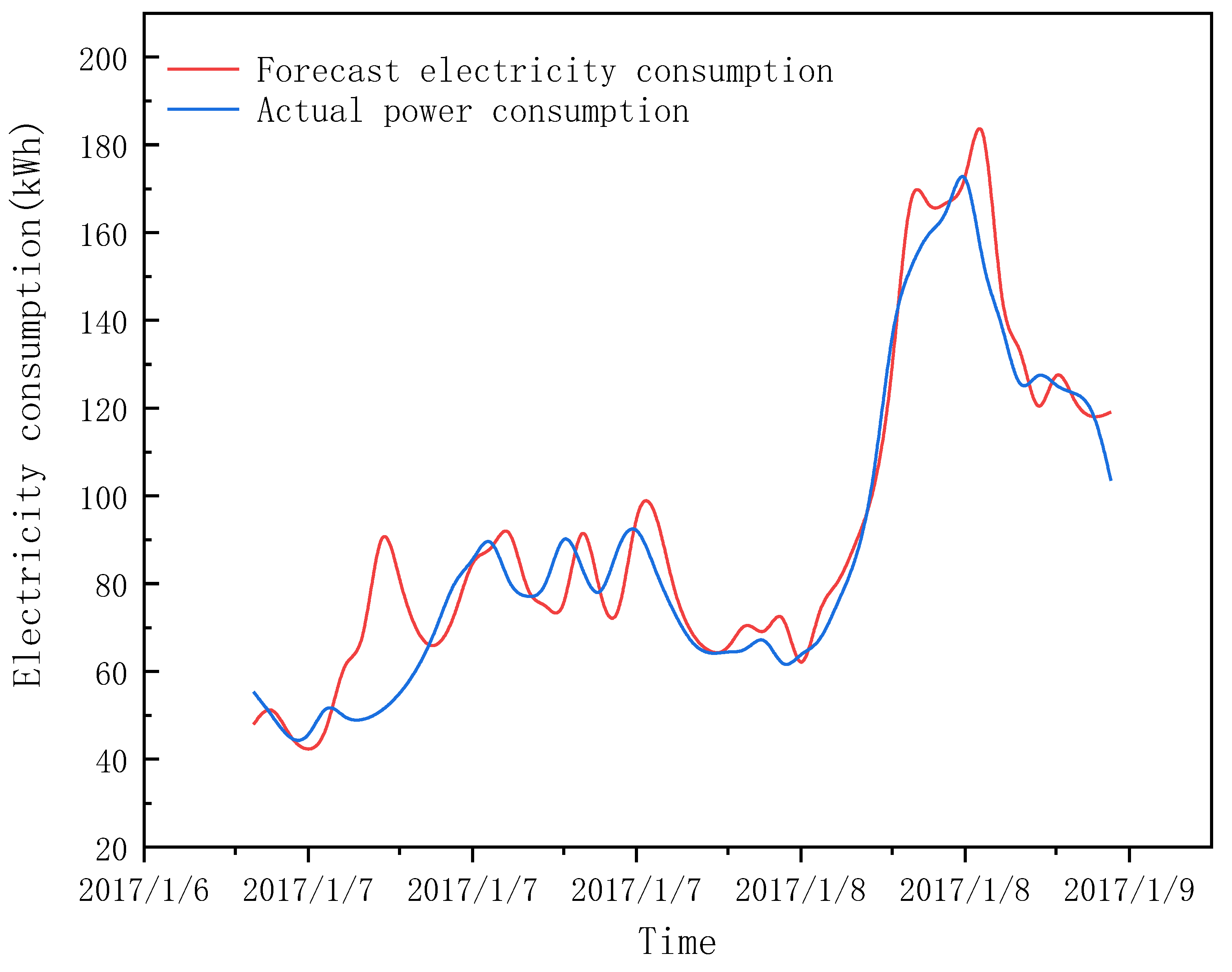
It is feasible to use the LSTM method to train the hourly electricity consumption data of the first two years to predict the hourly electricity consumption data of the office building in the next year, and the model has better prediction accuracy. However, the prediction accuracy of the model for air-conditioning electricity consumption is not so high, and the error of the prediction mainly appears in the morning from 7:00 to 8:00 on weekdays.

(2)

To further improve the air-conditioning prediction accuracy, we considered adding three other variables for model verification. When the dry bulb temperature is added as an input variable for prediction, the prediction accuracy decreases. This may be because the power consumption of the air conditioner is also affected by the building envelope; thus, the temperature has no direct influence on the power consumption of the air conditioner. When adding the “schedule” and “relative humidity” as input variables for prediction, the prediction accuracy can be slightly improved. This conclusion can be applied to other office buildings.

(3)

The increase in the accuracy of forecasting with the addition of other variables is mainly due to the improvement of the forecasting accuracy at the beginning of working hours (7 a.m.–8 a.m.) on weekdays, not the improvement of the accuracy of peak load forecasting.

(4)

Using the LSTM model, the prediction of lighting power consumption is very accurate, and only using historical power consumption data can well predict the lighting power consumption of buildings.

This study uses the LSTM method to verify that the model formed using the variables of historical electricity consumption data, schedule, and relative humidity has the greatest prediction accuracy. Whether this conclusion applies to all office buildings requires further verification. According to the results discussed in this article, the prediction accuracy of the air-conditioning model should be further improved.

References

1. Lund, H.; Mathiesen, B.V. Energy system analysis of 100% renewable energy systems—The case of Denmark in years 2030 and 2050. Energy 2009, 34, 524–531. [Google Scholar] [CrossRef]
2. Mendizabal, M.; Heidrich, O.; Feliu, E.; García-Blanco, G.; Mendizabal, A. Stimulating urban transition and transformation to achieve sustainable and resilient cities. Renew. Sustain. Energy Rev. 2018, 94, 410–418. [Google Scholar] [CrossRef]
3. Wei, Y.; Zhang, X.; Shi, Y.; Xia, L.; Pan, S.; Wu, J.; Han, M.; Zhao, X. A review of data-driven approaches for prediction and classification of building energy consumption. Renew. Sustain. Energy Rev. 2018, 82, 1027–1047. [Google Scholar] [CrossRef]
4. Moradi, M.; Dyer, B.; Nazem, A.; Nambiar, M.K.; Nahian, M.R.; Bueno, B.; Mackey, C.; Vasanthakumar, S.; Nazarian, N.; Krayenhoff, E.S.; et al. The Vertical City Weather Generator (VCWG v1.3.2). Geosci. Model Dev. 2021, 14, 961–984. [Google Scholar] [CrossRef]
5. Zhang, L.; Wen, J.; Li, Y.; Chen, J.; Ye, Y.; Fu, Y.; Livingood, W. A review of machine learning in building load prediction. Appl. Energy 2021, 285, 116452. [Google Scholar] [CrossRef]
6. Aliabadi, A.A.; Moradi, M.; McLeod, R.M.; Calder, D.; Dernovsek, R. How Much Building Renewable Energy Is Enough? The Vertical City Weather Generator (VCWG v1.4.4). Atmosphere 2021, 12, 882. [Google Scholar] [CrossRef]
7. Ahmad, M.I. Seasonal Decomposition of Electricity Consumption Data. Rev. Integr. Bus Econ. Res. 2017, 6, 271–275. [Google Scholar]
8. Li, X.; Wen, J. Review of building energy modeling for control and operation. Renew. Sustain. Energy Rev. 2014, 37, 517–537. [Google Scholar] [CrossRef]
9. Fumo, N. A review on the basics of building energy estimation. Renew. Sustain. Energy Rev. 2014, 31, 53–60. [Google Scholar] [CrossRef]
10. Pan, S.; Wang, X.; Wei, Y.; Zhang, X.; Gal, C.; Ren, G.; Yan, D.; Shi, Y.; Wu, J.; Xia, L.; et al. Cluster analysis for schedule based electricity load patterns in buildings: A case study in Shanghai residences. Build. Simul. 2017, 10, 889–898. [Google Scholar] [CrossRef]
11. Niu, F.; O’Neill, Z.; O’Neill, C. Data-driven based estimation of HVAC energy consumption using an improved Fourier series decomposition in buildings. Build. Simul. 2018, 11, 633–645. [Google Scholar] [CrossRef]
12. De Nadai, M.; Van Someren, M. Short-term anomaly detection in gas consumption through ARIMA and Artificial Neural Network forecast. In Proceedings of the 2015 IEEE Workshop on Environmental, Energy, and Structural Monitoring Systems (EESMS 2015), Trento, Italy, 9–10 July 2015; pp. 250–255. [Google Scholar] [CrossRef]
13. Wang, J.Q.; Du, Y.; Wang, J. LSTM based long-term energy consumption prediction with periodicity. Energy 2020, 197, 117197. [Google Scholar] [CrossRef]
14. Valgaev, O. Building Power Demand Forecasting Using K-Nearest Neighbors Model—Initial Approach. In Proceedings of the 2016 IEEE PES Asia-Pacific Power and Energy Engineering Conference (APPEEC), Xi’an, China, 25–28 October 2016; pp. 1055–1060. [Google Scholar]
15. Li, Z.; Dai, J.; Chen, H.; Lin, B. An ANN-based fast building energy consumption prediction method for complex architectural form at the early design stage. Build. Simul. 2019, 12, 665–681. [Google Scholar] [CrossRef]
16. Ferlito, S.; Atrigna, M.; Graditi, G.; De Vito, S.; Salvato, M.; Buonanno, A.; Di Francia, G. Predictive models for building’s energy consumption: An Artificial Neural Network (ANN) approach. In Proceedings of the 2015 Xviii Aisem Annual Conference, Trento, Italy, 3–5 February 2015; pp. 3–6. [Google Scholar]
17. Ahmad, A.S.; Hassan, M.Y.; Abdullah, M.P.; Rahman, H.A.; Hussin, F.; Abdullah, H.; Saidur, R. A review on applications of ANN and SVM for building electrical energy consumption forecasting. Renew. Sustain. Energy Rev. 2014, 33, 102–109. [Google Scholar] [CrossRef]
18. Zhao, H.X.; Magoulès, F. A review on the prediction of building energy consumption. Renew. Sustain. Energy Rev. 2012, 16, 3586–3592. [Google Scholar] [CrossRef]
19. Dong, B.; Cao, C.; Eang, S. Applying support vector machines to predict building energy consumption in tropical region. Energy Build. 2005, 37, 545–553. [Google Scholar] [CrossRef]
20. Wang, Z.; Hong, T.; Piette, M.A. Building thermal load prediction through shallow machine learning and deep learning. Appl. Energy 2020, 263, 114683. [Google Scholar] [CrossRef] [Green Version]
21. Salehinejad, H.; Sankar, S.; Barfett, J.; Colak, E.; Valaee, S. Recent Advances in Recurrent Neural Networks. arXiv 2017, arXiv:1801.01078. [Google Scholar]
22. Fan, C.; Xiao, F.; Zhao, Y. A short-term building cooling load prediction method using deep learning algorithms. Appl. Energy 2017, 195, 222–233. [Google Scholar] [CrossRef]
23. Sendra-Arranz, R.; Gutiérrez, A. A long short-term memory artificial neural network to predict daily HVAC consumption in buildings. Energy Build. 2020, 216, 109952. [Google Scholar] [CrossRef]
24. Zhou, C.; Fang, Z.; Xu, X.; Zhang, X.; Ding, Y.; Jiang, X. Using long short-term memory networks to predict energy consumption of air-conditioning systems. Sustain. Cities Soc. 2020, 55, 102000. [Google Scholar] [CrossRef]
25. Satre-Meloy, A.; Diakonova, M.; Grünewald, P. Cluster analysis and prediction of residential peak demand profiles using occupant activity data. Appl. Energy 2020, 260, 114246. [Google Scholar] [CrossRef]
26. Dutilleul, P.; Stockwell, J.D.; Frigon, D.; Legendre, P. The Mantel test versus Pearson’s correlation analysis: Assessment of the differences for biological and environmental studies. J. Agric. Biol. Environ. Stat. 2000, 5, 131–150. [Google Scholar] [CrossRef]
27. Adhianto, L.; Banerjee, S.; Fagan, M.; Krentel, M.; Marin, G.; Mellor-Crummey, J.; Tallent, N.R. HPCTOOLKIT: Tools for performance analysis of optimized parallel programs. Concurr. Comput. Pract. Exp. 2010, 22, 685–701. [Google Scholar] [CrossRef]
28. Kim, T.Y.; Cho, S.B. Predicting residential energy consumption using CNN-LSTM neural networks. Energy 2019, 182, 72–81. [Google Scholar] [CrossRef]
29. Wangpattarapong, K.; Maneewan, S.; Ketjoy, N.; Rakwichian, W. The impacts of climatic and economic factors on residential electricity consumption of Bangkok Metropolis. Energy Build. 2008, 40, 1419–1425. [Google Scholar] [CrossRef]
30. Peng, L.; Liu, S.; Liu, R.; Wang, L. Effective long short-term memory with differential evolution algorithm for electricity price prediction. Energy 2018, 162, 1301–1314. [Google Scholar] [CrossRef]
31. Huang, L.; Wang, J. Global crude oil price prediction and synchronization based accuracy evaluation using random wavelet neural network. Energy 2018, 151, 875–888. [Google Scholar] [CrossRef]
Figure 1. Violin chart of the meteorological parameters.
Energies 14 04785 g001
Figure 2. Monthly electricity consumption for air conditioning and lighting in a high-rise office from 2015 to 2017.
Energies 14 04785 g002
Figure 3. Distribution diagram of the electricity consumption data.
Energies 14 04785 g003
Figure 4. LSTM structure compared with an ordinary RNN.
Energies 14 04785 g004
Figure 5. Algorithm structure of LSTM.
Energies 14 04785 g005
Figure 6. Different model daily air-conditioning electricity forecast results in 2017.
Energies 14 04785 g006
Figure 7. Hourly air-conditioning electricity forecast in 2017.
Energies 14 04785 g007
Figure 8. Air-conditioning electricity forecast in 2017.
Energies 14 04785 g008
Figure 9. Forecast of air conditioning power consumption in summer 2017.
Energies 14 04785 g009
Figure 10. Forecast of air conditioning energy consumption in winter working days.
Energies 14 04785 g010
Figure 11. Forecast of air conditioning energy consumption on non-working days in winter.
Energies 14 04785 g011
Figure 12. Forecast of the air-conditioning electricity consumption on a working day.
Energies 14 04785 g012
Figure 13. Hourly lighting electricity forecast in 2017.
Energies 14 04785 g013
Figure 14. Forecast of air-conditioning energy consumption in a week.
Energies 14 04785 g014