1. Introduction
The radiant cooling panel (RCP) system has become one of the solutions to improving indoor thermal comfort, due to its low energy consumption compared to all-air systems [
1]. RCP provides extensive flexibility in terms of installation and zoning compared to other radiant system types, such as thermally active building systems (TABS) and capillary tube systems, which have tubes embedded in the concrete layer of the building structure [
2]. RCP can easily be placed on the ceiling of the building, as well as on the wall column inside a room. Because of the ease of installation, RCP can be used in both new and retrofitted buildings [
2].
However, the radiant cooling (RC) system has a condensation problem that hinders the widespread growth of this new technology [
3]. The high risk of surface condensation limits the usage of radiant cooling in hot and humid areas [
2]. In order to prevent the risk of surface condensation, the supply water temperature should be higher than the dew point temperature of the air inside the room [
1]. However, by increasing the supply water temperature, the cooling power of the radiant cooling system will not perform to its full potential [
1]. Therefore, research into RCP flow configurations is vital to achieving the maximum cooling potential of the system.
S. Oubenmoh et al. [
4] conducted a numerical investigation on the effect of pipe arrangement on RCP performance. The design considerations chosen for the investigation are counterflow, serpentine, and modulated spiral. It is noticeable that the tubing’s geometry influences the average temperature of the core surface where each of the pipe arrangements produces a different maximum core surface temperature. In terms of pressure losses, the modulated spiral configuration exhibits the lowest pressure losses across the pipe, with better thermal homogeneity. The energy consumption of the pump can further be reduced by reducing the inlet water velocities, but more considerations about the design and configuration should be taken into account.
M. Mosa et al. [
5] studied two design groups of RCP systems, these being serpentine flow configurations and canopy-to-canopy-flow configurations. The simulation carried out was intended to find the influence of the panel’s aspect ratio on the surface temperature distribution of the RCP. The aspect ratio is calculated as the width over the length of the RCP. A serpentine flow configuration with a higher aspect ratio exhibits greater pressure drop, due to the increasing number of bends over the serpentine tube’s total length. More pumping power is required on a serpentine tube that has higher aspect ratios. However, for the canopy-to-canopy flow configurations, the aspect ratio of the RCP does not influence the cooling performance of the RCP. M. Mosa et al. [
5] claim that the compactness in the RCP flow configuration can increase the ratio of cooling capacity per pumping power.
A multi-segmented mini-channel radiant ceiling cooling panel (MCRCP) is a new RCP design, as proposed by Lan Ding et al. [
6]. Five simulation scenarios are conducted to analyze the relationship between the MCRCP panel area and its cooling performance. MCRCP panels with aspect ratios of 1.5, 2, 2.5, 3 and 4 are chosen for analysis. Based on the findings of Lan Ding et al. [
6], the cooling capacity of the MCRCP increases when the aspect ratio of the panel increases from 1 to 3. Further increasing the aspect ratio of the panel will result in decreasing the cooling capacity; the distance between the radiant panels becomes narrower, hindering the natural convection flow of the inside air [
6].
Although the research on RCP flow configurations has made some progress, studies on the dynamic changes of the RCP flow configurations on the cooling performance of the RCP are still limited. There is still a wide range of flow configurations that should be explored and implemented in the RCP system. A more uniform temperature distribution with minimum pressure drop will be likely to have better cooling capacity and efficiency. Therefore, it is expected that different flow configurations will demonstrate different performances in RCP systems.
In this work, a study on the implementation of a different flow configuration on the RCP, other than the conventional serpentine flow configuration, is conducted. The novelty of this study is to evaluate the cooling performance of the conventional serpentine flow configuration, and different designs are compared under similar flow and thermal conditions. Innovative flow patterns for the serpentine-based designs are created by using the constructible approach, where the flow passage is varied in the RCP design, mainly by increasing the flow passages for the chilled water to pass through the RCP. The objective of this research is to analyze the cooling capacity, temperature distribution, and pressure drop of the RCP for each of the designs. The results from this research could provide technical information for the development of new RCP serpentine-based flow configurations.
The paper is categorized as follows. In
Section 2, proposed methods are presented. In
Section 3, the results and discussions of the proposed RCP are discussed.
Section 4 presents the authors’ findings and their conclusions.
2. Methods
This research focuses on the numerical simulation of three types of pipe arrangement configurations of the RCP, by varying the number of inlets and outlets of the serpentine flow configurations.
2.1. Computational Fluid Dynamics (CFD)
This research will be conducted using computational fluid dynamics (CFD) software, known as Ansys Fluent [
7,
8]. The Ansys Fluent software is used to simulate the fluid flow and investigate the heat transfer characteristics for different pipe arrangement configurations of the RCP. The Ansys Fluent software uses the Navier Stokes equation in the finite volume method (FVM) to analyze the results of the simulation [
9,
10].
The steady-state continuity equation, momentum conservation equation, and energy conservation equation are solved by Ansys Fluent with the basic governing equations described below [
11,
12]:
The continuity equation is shown in Equation (1), where
u, v and
w are the velocity component in
x, y and
z directions, respectively.
The momentum conservation equation in three dimensions is shown in Equations (2)–(4).
The energy conservation equation is shown in Equation (5), where
T is the fluid temperature,
ui is the velocity in different directions in Cartesian coordinates,
xi is the Cartesian coordinates,
k is the thermal conductivity,
Cp is the constant-pressure specific heat of fluid, and
ST is the radiative energy source term [
11,
13].
The Navier–Stokes equations are then transferred into discretized form for numerical solution. By using the FVM, the general form of the Navier–Stokes equation is integrated over a control volume, and the Gauss divergence theorem is applied. Equation (6) is used as a starting point for computational procedures in the FVM [
12].
ϕ is introduced as a general variable for the conservative form of all fluid flow equations [
12]:
where
is the rate of increase of the
ϕ fluid element,
is the net rate of flow of
ϕ out of the fluid element,
is the rate of increase of
ϕ due to diffusion, and
is the rate of increase of
ϕ due to the source terms.
The computational domain is divided into a finite number of close-proximity control volumes as discrete elements. They are located in the centroid of the control volume, and are called variables of interest [
14]. FVM uses interpolation to integrate the differential forms of the governing equations, to create discretized equations [
14]. The general discretized equation for interior nodes in three dimensions is shown in Equation (7) [
12]:
where Σ is the diffusion summation of all neighboring nodes (
nb) and
anb is for the neighboring coefficients.
ϕnb and
Su are the values of
ϕ at the neighboring nodes and linearized source term, respectively. The equation is mainly used in mesh grid sizing and grid spacing and will drastically affect the quality of the mesh. High-quality mesh can be produced by using Ansys Fluent, as the meshing runs the Navier–Stokes equation in a form of Fourier series. By using Ansys Fluent for this research, FVM is used for the generation of mesh, to find the cooling characteristics of the RCP.
2.2. Pipe Arrangement Configurations
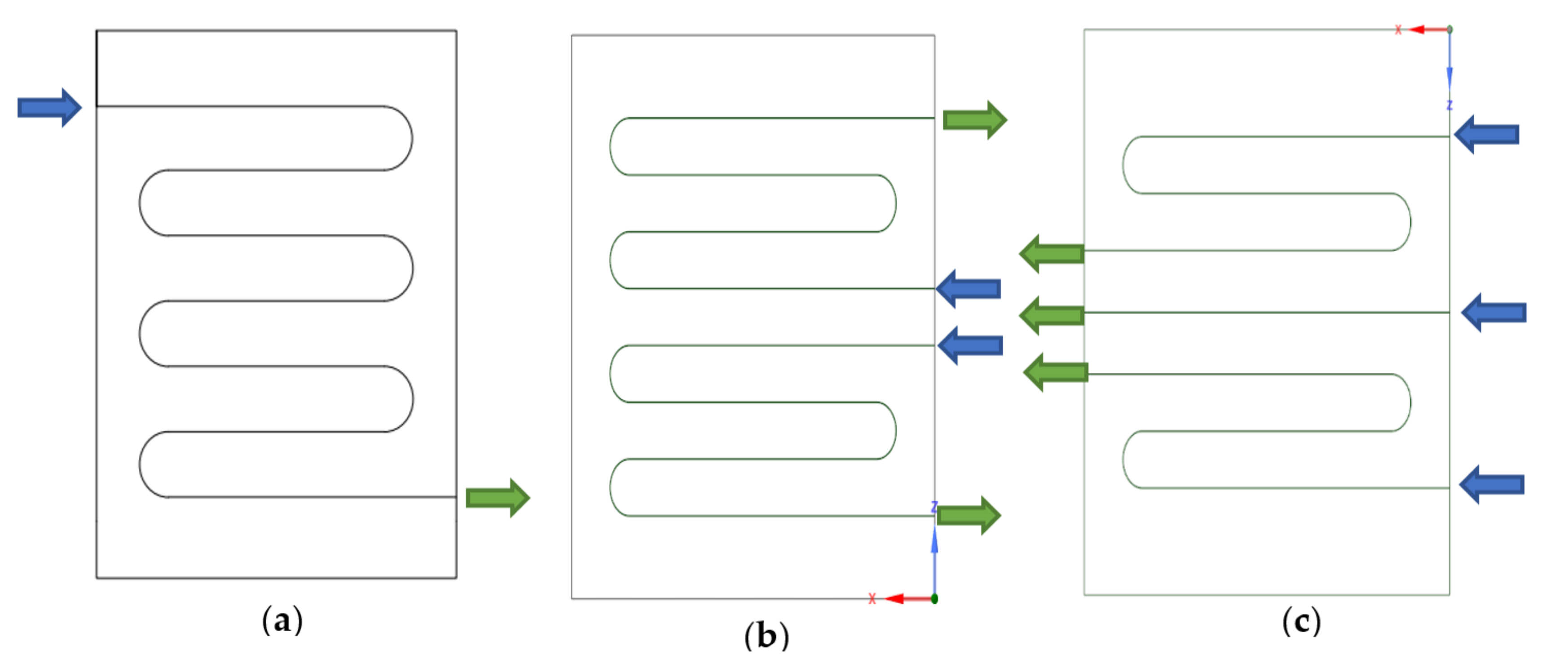
Figure 1a–c shows the proposed designs of the pipe arrangement configuration that will be used in this research.
Figure 1a is the common serpentine flow configuration and is widely used with RCP [
1,
15,
16,
17,
18,
19,
20,
21,
22].
Figure 1a will serve as a benchmark for the other two proposed designs. The design of
Figure 1b is known as a counterflow serpentine, with two-inlet-two-outlet flow configurations, while
Figure 1c is a serpentine design with three-inlet-three-outlet flow configurations. The relevancy of the number of inlet and outlet flows for an RCP is determined by studying the three proposed designs.
2.3. Mathematical Model
Based on the sketch in
Figure 1, chilled water flows from the inlet of the copper tube and goes through the channels of the tube. The top and sides of the radiant panel are insulated, and heat flux is applied from beneath the radiant panel. Therefore, heat exchange occurs between the aluminum plate and the chilled water flowing through the copper tube. The fluid inlet temperature and ambient temperature are kept constant throughout the simulation. The plate area and flow volume are defined as Equations (8) and (9).
where
W and
L is the width (m) and length of the plate (m), respectively.
D is the tube diameter (m) and
Ltube is the flow path length (m). The governing equations for the model are shown in Equations (1)–(5).
The total heat flux received by the panel is expressed by Equation (10). The total heat flux is the summation of radiation and convection heat transfer between the surrounding temperature and the panel’s surface.
where
hr is the radiation heat transfer coefficient,
AUST is the area-weighted average temperature of all the uncontrolled surfaces in the conditioned space,
Tp is the effective radiant panel surface temperature and
hc is the convection heat transfer coefficient. The equation for radiation and convection heat transfer coefficient is expressed as shown in Equations (11) and (12), respectively [
23]:
where σ is the Stephan–Boltzmann constant, and
is the radiation interchange factor between the panel surface temperature and
jth surface temperature,
Tj.
where
Tamb is the ambient air temperature.
However, based on data from the American Society of Heating, Refrigerating and Air-Conditioning Engineers (ASHRAE), the radiation and convective heat fluxes for a suspended RCP may also be estimated by using Equations (13) and (14) [
24]:
For the calculation of heat flux, an initial value of plate temperature,
Tp, is needed to be assumed and adjusted accordingly throughout the simulation.
AUST is assumed to be the same as
Tamb for ease of calculation, normally when the cases and design adhere to ASHRAE 1999a [
16,
25].
Table 1 below shows the heat transfer characteristics, based on the mean panel temperature determined by Mumma et al. [
25].
2.4. Material Properties
The thermophysical properties of the elements found in the RCP are given in
Table 2 [
26].
2.5. Simulation Domain and Boundary Conditions
The boundary conditions are taken from real conditions selected from other research papers. The boundary conditions and domains are obtained from [
1,
5] and are summarized as shown in
Table 3.
The boundary conditions are as follows:
- (a)
The mass flow rate at the pipe inlet is 0.004 kg/s, with a temperature of 15 °C.
- (b)
The top and sides of the radiant panel are insulated.
- (c)
Heat flux is applied from underneath the radiant panel as it is exposed to room temperature.
- (d)
The ambient air temperature is assumed to be 24 °C.
There are also some assumptions made to simplify the simulation model. The assumptions are as follows:
- (a)
The flow inside the copper tube is laminar and incompressible.
- (b)
The pipe wall thickness is proposed to be a thin layer, as the thermal conductivity of copper is high, and the wall thickness is very small. Therefore, the wall thickness is ignored.
- (c)
The aluminum panel has perfect contact with the copper tube.
2.6. Operating Conditions and Design Parameters
Based on M. Mosa et al. [
5], a radiant panel with a 1.05 aspect ratio gives the highest cooling capacity for the serpentine flow configuration. Therefore, this research uses the given aspect ratio of the radiant panel as a reference. Note that the aspect ratio is the width to length ratio of the RCP.
The values for the aspect ratio (
Ar), panel area (
Ap), width (
W), length (
L), panel thickness (
t), inner diameter (
Do), and outer diameter (
Di) of the copper tube are summarized in
Table 4. The values for the operating condition for water inlet temperature (
Tw,in), ambient temperature (
Tamb), water inlet mass flow rate (
ṁin), and area-weighted average temperature (
AUST) are also shown in
Table 4.
2.7. Geometrical Setup of the Proposed Design
The 3D design of the RCP model is created by using Autodesk Fusion 360. This software is used because it makes it easier to construct 3D modeling. The completed 3D design of the RCP is then converted into a
.step file. The
.step file of the design is then imported into SpaceClaim for flow simulation. The dimension of this model follows the parameters proposed in
Table 4. The generated model of a one-inlet-one-outlet serpentine flow configuration, as modeled by using Autodesk Fusion 360 in SpaceClaim, is shown in
Figure 2.
After generating a 3D model of the RCP, a hexahedral mesh is used for the generation of mesh on the design model in
Figure 3. Hexahedral mesh is chosen because it enables a more accurate result on a simple geometry model. Edge sizing is used at the inlet and outlet flow of the fluid domain. The mesh is smoothed by applying 10, 15, 20 and 25 divisions on the mentioned edge for the grid independence test, to ensure that the grid size used is suitable to obtain a converged solution.
The simulation domains and boundary locations are specified after the mesh generation of the model is completed. The fluid domain is the pipe carrying chilled water, and the solid domain is the aluminum plate located below the fluid domain. Heat exchange will occur between the two domains, with the boundary conditions mentioned in
Table 3. The fluid domain is set to have the properties of water, and the solid domain has the properties of aluminum.
For the solver execution part, a laminar model is chosen because the calculated Reynolds number is in the laminar region. The energy equation is turned on as heat exchanges occur between the fluid domain and the solid domain. The solver type is pressure-based and steady-state. A steady-state simulation is faster than a transient one and is thus suitable for this study, to save time and computational load.
For the solution part, a Semi-Implicit Method for Pressure Linked Equations (SIMPLE) is used for the pressure-velocity coupling and is set as the solution method. A second-order upwind is chosen for the spatial discretization of the momentum and energy equations, whereas the gradient discretization is based on the least-squares cell, and pressure discretization is set as second-order. The residual tolerance used for continuity, x-velocity, y-velocity, z-velocity, and energy is 0.001, which is the default value from ANSYS Fluent. Hybrid initialization is used, and 1000 iterations are chosen to make sure that the value obtained is accurate and converged.
Finally, the results obtained in the post-processing stage are analyzed and examined for discussion. The results that will be taken for analysis are the temperature contour of the RCP, pressure contour, outlet water temperature, surface temperature of RCP, and pressure drop inside the tube. The cooling capacity and temperature distribution uniformity are determined from the surface temperature of the RCP.
The steps above will be repeated on the other two proposed designs of the RCP flow configurations.
2.8. Validation
In order to validate the CFD simulation, the convergence of the simulation result needs to be obtained. To further validate the CFD simulation, the results obtained are compared with other literatures
Table 5 shows the calculated results and experimental results of the RCP model obtained under constant indoor environmental factors. These data are taken from W. Jin et al. [
27] and Zhang et al. [
28], and are compared with the conventional serpentine flow configuration results. Based on the comparisons, the outlet water temperature and the surface panel temperature of the RCP differ slightly from the simulated conventional serpentine. The percentage errors of the outlet water temperature and surface panel temperature for comparison 1 are 4.30% and 5.33%, respectively, while the percentage errors for comparison 2 are 1.07% and 4.44%, respectively. The error caused is mainly because of the different inlet water temperatures used for the simulation. Nevertheless, the error obtained for both of the comparisons is within 5%, which is acceptable for engineering applications. Therefore, the experimental results from [
27,
28], as well as the temperature contour obtained, verified the simulation result of the conventional serpentine flow configuration.
3. Results and Discussions
3.1. Grid Independence Test
A grid independence test was carried out on Design 1 (see
Figure 1a) to determine the best number of elements required for the simulation.
Table 6 shows the grid independence test result, where the number of elements is the variable, and the pressure drop and outlet temperature are taken for analysis.
In the grid independence test analysis, the operating conditions and parameters were kept constant, while the number of meshing elements was varied. Based on the graph presented in
Figure 4 and
Figure 5, the outlet temperature became constant as the number of elements increased, while the pressure drop did not seem to be affected greatly by the number of elements, since the result was showing a consistent value with a 0.0337 variance. Therefore, the total number of elements used in the simulation was chosen to be 313,492, since the outlet temperature began to converge into a steady value while there was negligible variation in the pressure drop at this number of elements. Choosing a larger number of elements would only increase the computing time, without any significant impact on the simulation.
3.2. CFD Simulation—ANSYS Fluent
The results obtained from the simulations conducted for all three proposed flow configurations (
Figure 1a–c) of the RCP are shown in this section. All the designs simulated have achieved a converged solution, where the solution is unique and, therefore, can be used for further analysis.
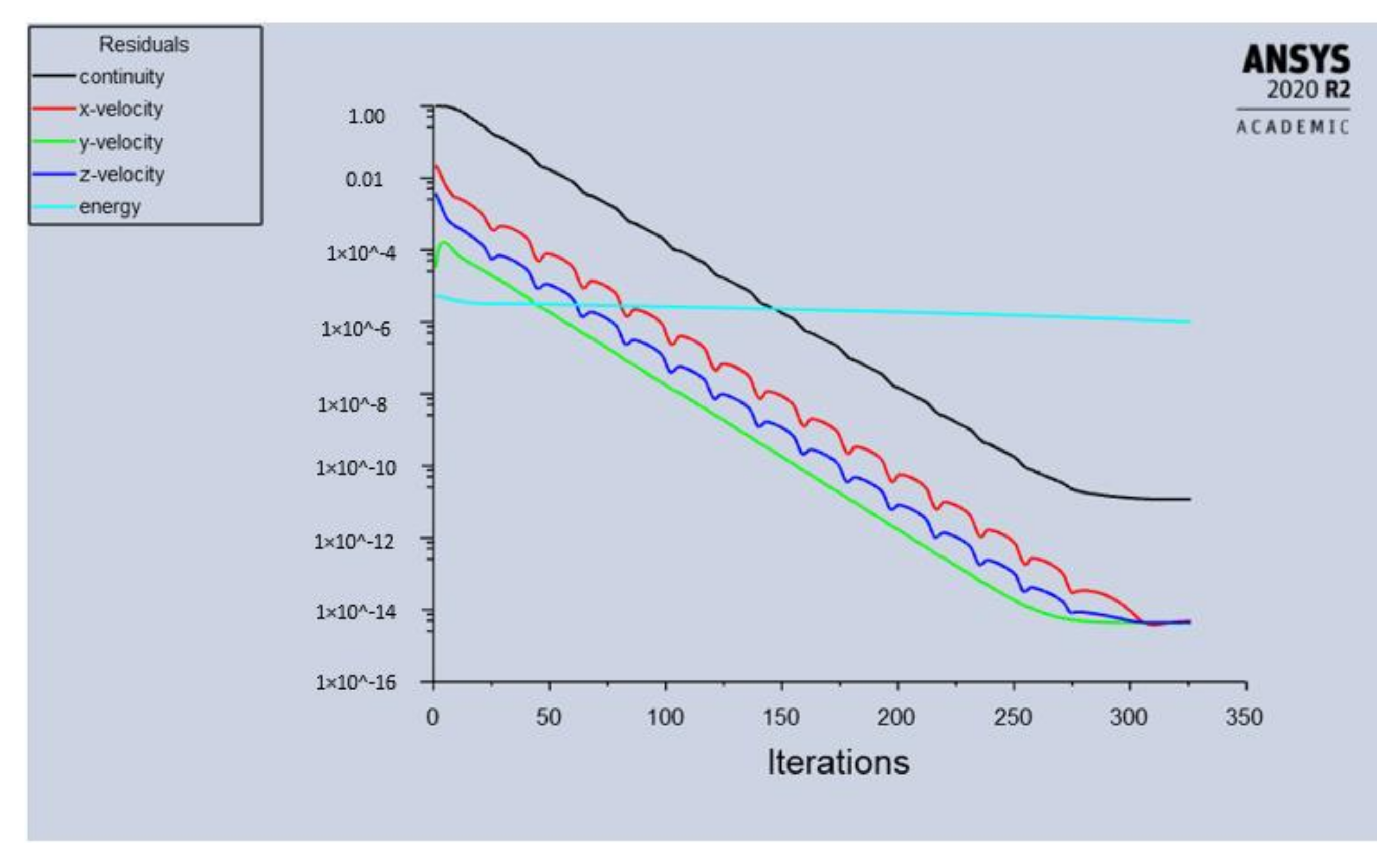
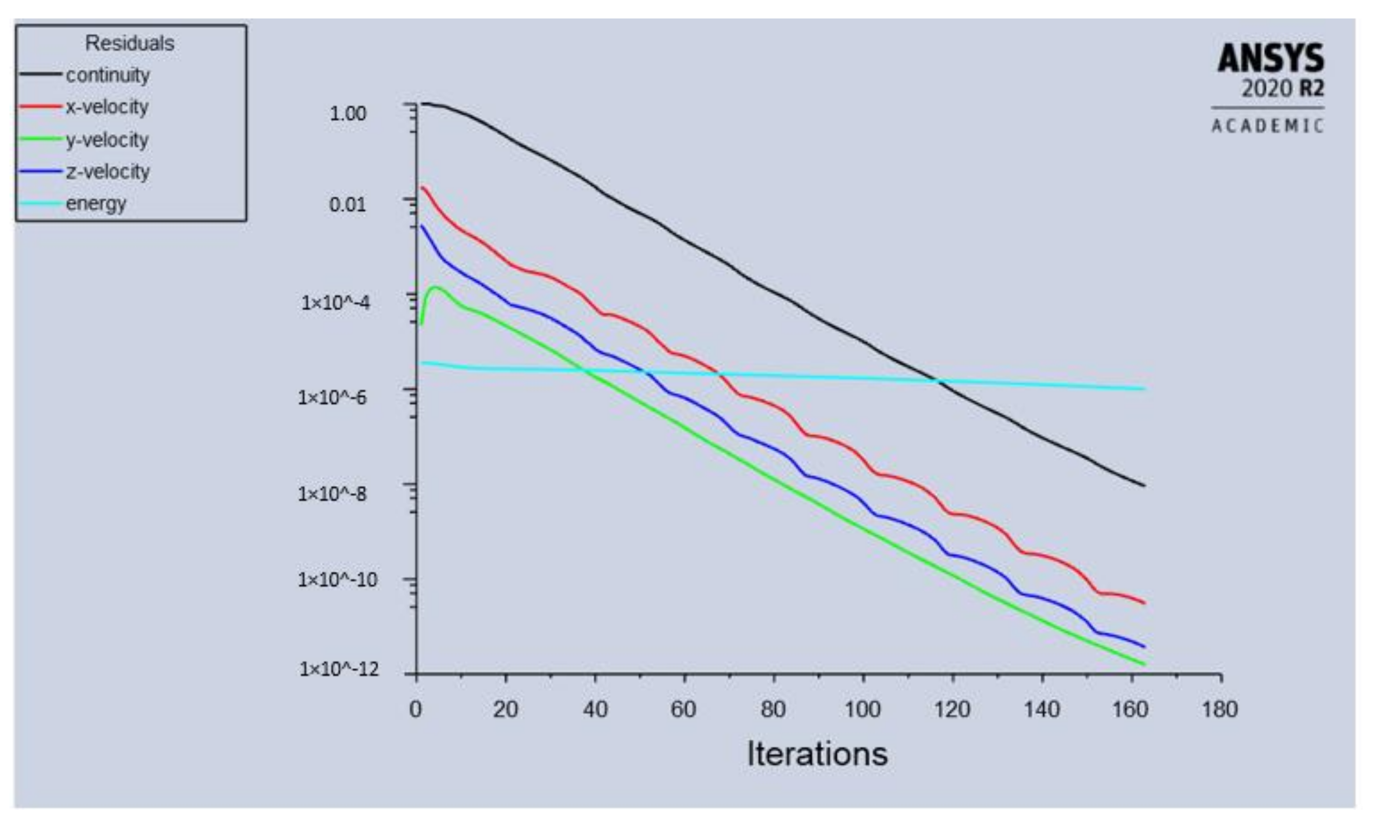
3.2.1. Residual Plot
Figure 6,
Figure 7 and
Figure 8, below, show the residual plot for all three flow configurations. Here, they are denoted as Design 1, Design 2 and Design 3 for
Figure 1a–c, respectively. A residual plot is important in determining the reliability of the simulation result. In the simulations conducted, all the flow configurations have achieved convergence and, therefore, the results of the simulation can be considered accurate, with low residual error.
3.2.2. Temperature Contour and Pressure Contour
Temperature contour and pressure contour for all three flow configurations, obtained from the simulations, are shown in
Figure 9 and
Figure 10.
3.3. Analysis and Discussions
The findings obtained from the simulation results are further analyzed in this section. This includes the analysis of the temperature distribution of the RCP with different serpentine flow configurations. In addition, the pressure drop inside the tube is identified based on the simulation. Moreover, important parameters, such as outlet water temperatures, minimum and maximum plate temperature, as well as the average plate temperature, are obtained and analyzed for each of the serpentine flow configurations.
3.3.1. Maximum Outlet Water Temperature and Total Heat Transfer Heat
Based on the results obtained from the simulations, all the maximum temperatures and total heat transfer rate for each serpentine flow configuration are tabulated in
Table 6 below, with the water inlet temperature, T
inlet = 288 K.
Based on
Table 7, Design 2, with the two-inlet-two-outlet serpentine flow configuration, has the highest maximum rate of heat transfer with the maximum temperature of 289.716 K at outlet 1, and 289.727 K at outlet 2. The temperature difference at outlet 1 is 1.716 K and 1.727 K at outlet 2, with a total heat transfer of 28.111 W. Based on the simulation results, heat is absorbed equally between the two pipes in Design 2, resulting in a lower temperature difference with a higher total heat transfer rate. In the case of Design 3, the middle pipe, which is outlet 2, has only 1130 mm of pipe length, resulting in a lower performance of heat absorption from the panel surface.
3.3.2. Temperature Distribution
Table 8 shows the minimum and maximum temperatures of the panel’s surface, with its mean panel temperature as calculated by Ansys Fluent.
Based on
Table 8, Design 2 has the lowest mean panel temperature, indicating that the temperature distribution in Design 2 has the most uniformity. The common serpentine flow configuration in Design 1 has the highest mean panel temperature, with a 298.919 K maximum panel temperature and a 293.441 K minimum panel temperature. Based on the panel’s surface temperature, shown in
Table 8, Design 1 is not as good as the other two designs in respect of obtaining uniform temperature distribution. This is because the water flowing inside the tube becomes hotter with the increasing length, thus decreasing the heat absorption performance, resulting in a higher panel temperature at the area around the water outlet. This phenomenon can be seen from the temperature contour shown in
Figure 9, where the edge of the panel surface located at the water outlet has a higher temperature compared to the panel surface located near the water inlet. The concentration of the cold region can be seen clearly at the water inlet, with temperature increases along the pipe length. This temperature contour agrees with Mohamed Mosa et al. [
1] showing a similar temperature distribution characteristic.
In the case of Design 2, the cold region is concentrated in the middle part of the RCP. This is because the water inlets are located next to each other, thus creating a very low minimum panel surface temperature at that region. In addition, the temperature contour for Design 2 shows a uniform temperature distribution throughout the panel’s surface compared to those of Design 1 and Design 3. There is a smaller greenish region observed in the temperature contours of both Design 1 and Design 3. What is more, the greenish region that represents a relatively low-temperature zone is not evenly spread throughout the panel’s surface in both Design 1 and Design 3.
The middle pipe has no significant impact on the cooling performance of the RCP in Design 3, and the cold region is only concentrated at the right side of the panel’s surface where the water inlet is located. The left side of the panel’s surface, where the water outlets are placed near each other, shows an increase in temperature due to the increase of water temperature being concentrated in that region.
For all three designs, the tubes did not cover the edges of the plate, resulting in a hotter region compared to the rest of the surface [
1]. This is because the chilled water has less access to the surface of those regions [
1]. To gain more understanding of the temperature distribution of the panel’s surface, a temperature distribution graph is plotted by dividing the plate into three equally spaced segments. The plate is divided into the right-hand side, middle, and left-hand side of the plate in the graphical analysis shown in
Figure 11,
Figure 12 and
Figure 13.
By comparing the three temperature distribution graphs, it can be seen that Design 1 has the least temperature distribution uniformity where the plotted temperature for each segment is not concentrated in the same location, unlike in Design 2. Although the minimum, maximum, and mean plate temperatures in Design 3 do not differ that much from those of Design 2, the temperature distribution graph shows that the temperature is not distributed uniformly throughout the plate.
In terms of calculation, the temperature difference of Design 2 is the lowest compared to those of Design 1 and Design 3 at 4.505 °C, whereas Design 1 and Design 3 have a temperature difference of 5.478 °C and 5.175 °C, respectively. A smaller temperature difference indicates that the temperature distribution of a particular radiant cooling panel has a higher uniformity because its temperature spread is limited to that specific range. From this finding, Design 2 shows the most promising result for temperature difference calculation, with the most concentrated temperature distribution graph plotted. Therefore, Design 2, with a two-inlet-two-outlet counterflow serpentine configuration, has the highest uniformity in terms of temperature distribution.
3.3.3. Cooling Capacity
The cooling capacity of the RCP for each of the flow configurations was analyzed and calculated by using Equations (13) and (14), as given in
Section 2.3. The cooling capacity formula was taken from ASHRAE Transactions [
29], where the apparent heat is removed from the room by convection and radiation, which is absorbed by the RCP. Therefore, the cooling capacity, the Q
cool of the RCP can be determined by calculating the total heat flux absorbed through radiation and convection.
Based on
Table 9, Design 2 had the highest cooling capacity compared to the other two designs. Design 1, which is the common serpentine flow configuration, had the lowest cooling capacity, which was 19.752 W/m
2 smaller than that of Design 2. Design 2 is created from a heat exchanger perspective, where counterflow is more efficient than a parallel flow. By implementing this idea into the RCP where the inlet and outlet are located on the same side of the plate, a significant improvement of its cooling performance was achieved. The cooling performance of the RCP agrees with Mohamed Mosa et al. [
1], where the counterflow design group is better than the conventional flow design group. Therefore, the arrangement of pipe configuration can have a significant impact on its cooling performance. In addition, the heat transfer characteristics obtained also agree with Miriel et al. [
30], where the heat absorption consists of 2/3 radiation and 1/3 convection of the total heat transfer.
3.3.4. Pressure Drop
Based on the pressure contour shown in
Figure 10, the pressure decreases from the upstream to the downstream region for all of the flow configurations. This is due to pressure losses along the flow in the pipe. Pressure drop is closely related to pumping power, meaning that the higher the pressure drop, the larger the pumping power needed to operate the system. Therefore, it is important for us to determine the total pressure drop in order to design a more efficient cooling system for the RCP.
The pressure drop is determined by using the Ansys Fluent post-processing method, and is compared to a manual calculation derived from Bernoulli’s equation for pressure drop [
31], as shown in Equation (16):
where
P1 is the static pressure at the inlet and
P2 is the static pressure at the outlet.
is the fluid velocity,
Z is the elevation,
hL is the total head loss,
ρ is the fluid density, and
g is the gravitational acceleration. The total head loss,
hL is determined by using Equation (17):
where
is the friction factor,
L is the pipe length,
D is the pipe diameter and
k is the loss coefficient value. Because the flow is laminar and the pipe is circular, the formula used to calculate the friction factor is shown in Equation (18) [
31]:
Equation (19) is the simplified Bernoulli’s equation, where the inlet velocity is assumed to be the same as the outlet velocity. The pipe configuration is horizontal, thus the change in potential energy is ignored. The loss coefficient value, k, is determined to be 0.2 because the pipe is circular and has a 180° bend.
Based on
Table 10, the theoretical value of pressure drop is almost identical to the simulated value obtained from the simulation. These data prove that the simulated pressure drop can be validated with the governing Bernoulli’s equation, as the results obtained have a very low percentage of error. Comparing the results among all the three designs, Design 1 has the most pressure drop across the pipe. This is because the pipe configuration in Design 1 has a total of six bends in a single, long pipe. Unlike Design 2, the pipe configuration is divided into two pipes, meaning that it has only three bends for each pipe. For Design 3, the middle pipe is a straight pipe without any bends, while the other two pipes have two bends each. Because of this, the middle pipe of Design 3 has the lowest pressure drop. As can be noticed from the pressure contour figure, the pressure drop of the last serpentine is less than the first serpentine, because of the decreasing pressure throughout the flow toward the outlet [
32,
33]. With the increasing number of bends of the pipe, a larger pressure drop across the pipe is observed, as shown in
Figure 14. Therefore, the pressure drop across the pipe is highly related to the number of bends and the path length of the fluid.
3.4. Analysis and Discussions
The simulation results presented in
Section 3.2 show that the cooling capacity of the RCP can be enhanced by manipulating the flow configurations of the RCP. It was found that the proposed flow configurations enhanced the cooling capacity of RCP by 172.57% for Design 2 and 125.03% for Design 3. The percentage increase is compared with the cooling capacity of Design 1, which is the conventional serpentine flow configuration that acts as a benchmark for the two proposed designs. The RCP operates in an enclosed environment, in which the air and all the surfaces are kept at a constant temperature. Chilled water enters the RCP at 15 °C, resulting in a temperature difference between the RCP and the conditioned surrounding. Heat exchanges occur between the RCP and the conditioned surroundings due to the temperature difference. From this natural phenomenon, the heat exchange that occurs is more efficient in Design 2 compared to Design 1 and Design 3, because Design 2 enables a more uniform temperature distribution with the highest cooling capacity.
As shown in Equation (15), the cooling capacity, which is also known as total heat flux, as absorbed by the RCP, is the summation of radiation and convection heat transfer between the surrounding temperature and the panel’s surface. Our results agree with ASHRAE’s definition of radiant systems, where the radiation heat transfer amounts to 60% of the total heat flux absorbed by the RCP. Thus, these results could be applied to develop new RCP flow configurations with maximum cooling potential, because the cooling capacity of RCP is often insufficient in hot and humid climates, due to condensation problems. If proper RCP flow configurations have been discovered, the required cooling capacity can be achieved at a relatively higher chilled water temperature.
Although the proposed flow configurations effectively enhanced the cooling capacity of the RCP, the simulated results are recommended for validation with an experimental investigation. As this research is only for a single panel, appropriate experimentation and testing conditions are necessary to find out the required number of panels that should be integrated and distributed over the ceiling for effective cooling. With a larger number of panels, a higher water flow rate is needed throughout the large radiant surface of the RCP. Therefore, proper experimental research is needed to evaluate the pumping power of these designs to determine their applicability.
4. Conclusions
The aim of this research is to develop CFD numerical simulations in order to test and simulate some basic design aspects of the RCP system. A three-dimensional model of the RCP is used to study the performance of the RCP, in terms of temperature distribution, cooling capacity, and pressure drop across the pipe. The study is conducted on three different pipe configurations, which are one-inlet-one-outlet serpentine, two-inlet-two-outlet counterflow serpentine, and three-inlet-three-outlets serpentine flow configurations. Under the assumed operating conditions, the main findings of this research are as follows:
The two-inlet-two-outlet counterflow serpentine flow configuration leads to better temperature uniformity. The best result in terms of low and uniform temperature distribution can be obtained with the counterflow design because it produces the lowest temperature difference of the panel’s surface temperature, with a 4.505 °C temperature difference.
The common serpentine flow configuration exhibits the lowest cooling performance, with the highest pressure drop across the pipe. The single pipe of the common serpentine flow configuration has a pressure drop of as much as 129.4225 Pa, which greatly influences the energy efficiency of the pump.
Pressure drops can be reduced by reducing the number of bends of the pipe, as the loss coefficient factor increases with every bend. Design 1 has six bends in a single long pipe, resulting in the highest total loss coefficient value, while Design 2 and Design 3 have fewer bends for each pipe. The pressure drop obtained is higher in a pipe that has a higher number of bends.
Increasing the number of inlets and outlets of the serpentine flow configuration may not make a significant impact on the cooling performance. However, the arrangement of the pipe configuration, such as the location of the inlets and outlets of the pipe and also the compactness of the pipe arrangement, may influence the cooling performance of the RCP.
It can be concluded that the common serpentine flow configuration does not give the best performance for the RCP. The common serpentine flow configuration exhibits the lowest cooling capacity, with 11.446 W/m2. The highest cooling capacity of 31.198 W/m2 is obtained from the two-inlet-two-outlet counterflow serpentine flow configuration. Both of the proposed flow configurations outperform the common serpentine flow configuration in terms of cooling capacity, temperature distribution, and pressure drop. Therefore, the cooling performance of RCP can be improved by implementing different flow configurations for the RCP.
Moreover, flow uniformity is a significant factor influencing the efficiency of any thermal system, including an RCP. Applying a different pipe configuration to the RCP will affect the flow uniformity and the temperature distribution uniformity. Therefore, an RCP should be designed with care to provide sufficient indoor cooling with maximum thermal comfort. In order to achieve this, it is recommended that more research be conducted on the design of RCP; there are many other innovative flow configurations that can be implemented in the RCP. The search for the best design of RCP is a never-ending journey as there is no limit to ideas. In the quest for an improved panel architecture, it is important for us to report and document the current results, as they can serve as guidance for future research. Conducting the numerical simulation by using a full version of Ansys Fluent is suggested, to eliminate any uncertainties from the meshing, so that grid-independent tests can be conducted with a larger number of elements. To further validate the energy efficiency of these three designs, future research plans will include experimental and simulation studies on energy consumption for the pumping power of the three designs.


 ,
, 


