
The Setting of Strength Parameters in Stability Analysis of Open-Pit Slope Using the Random Set Method in the Bełchatów Lignite Mine, Central Poland


Abstract
:1. Introduction
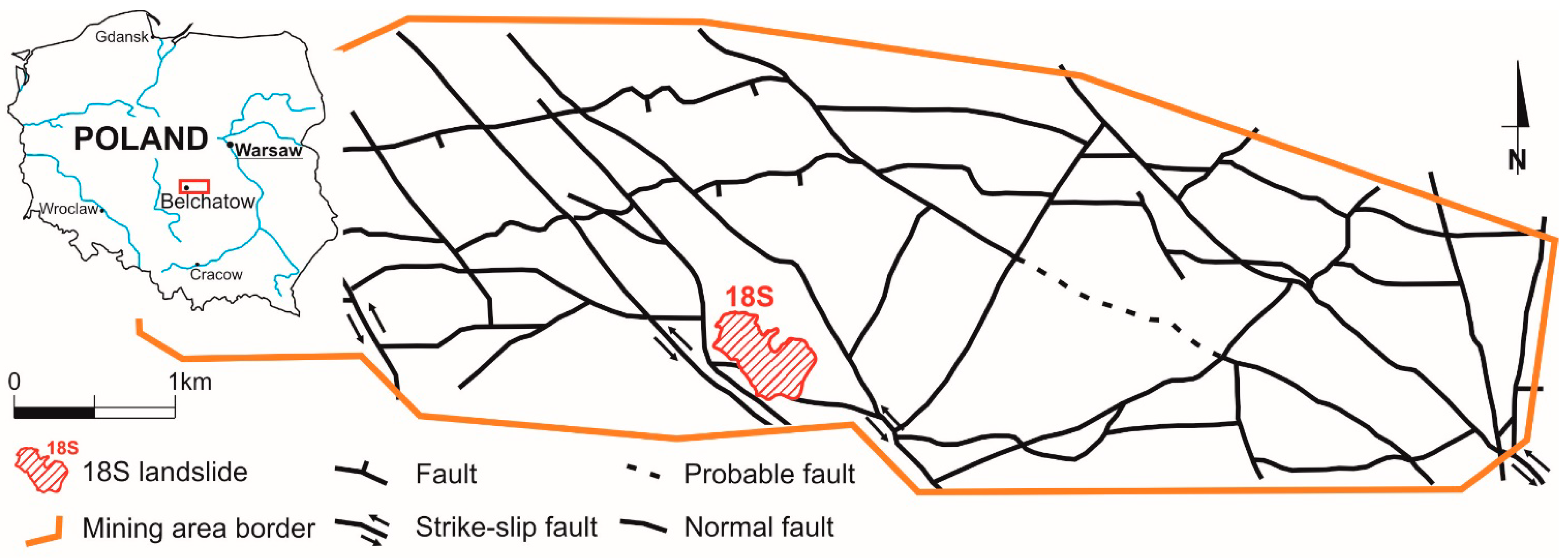
2. Geological and Mining Setting
3. Methods and Data
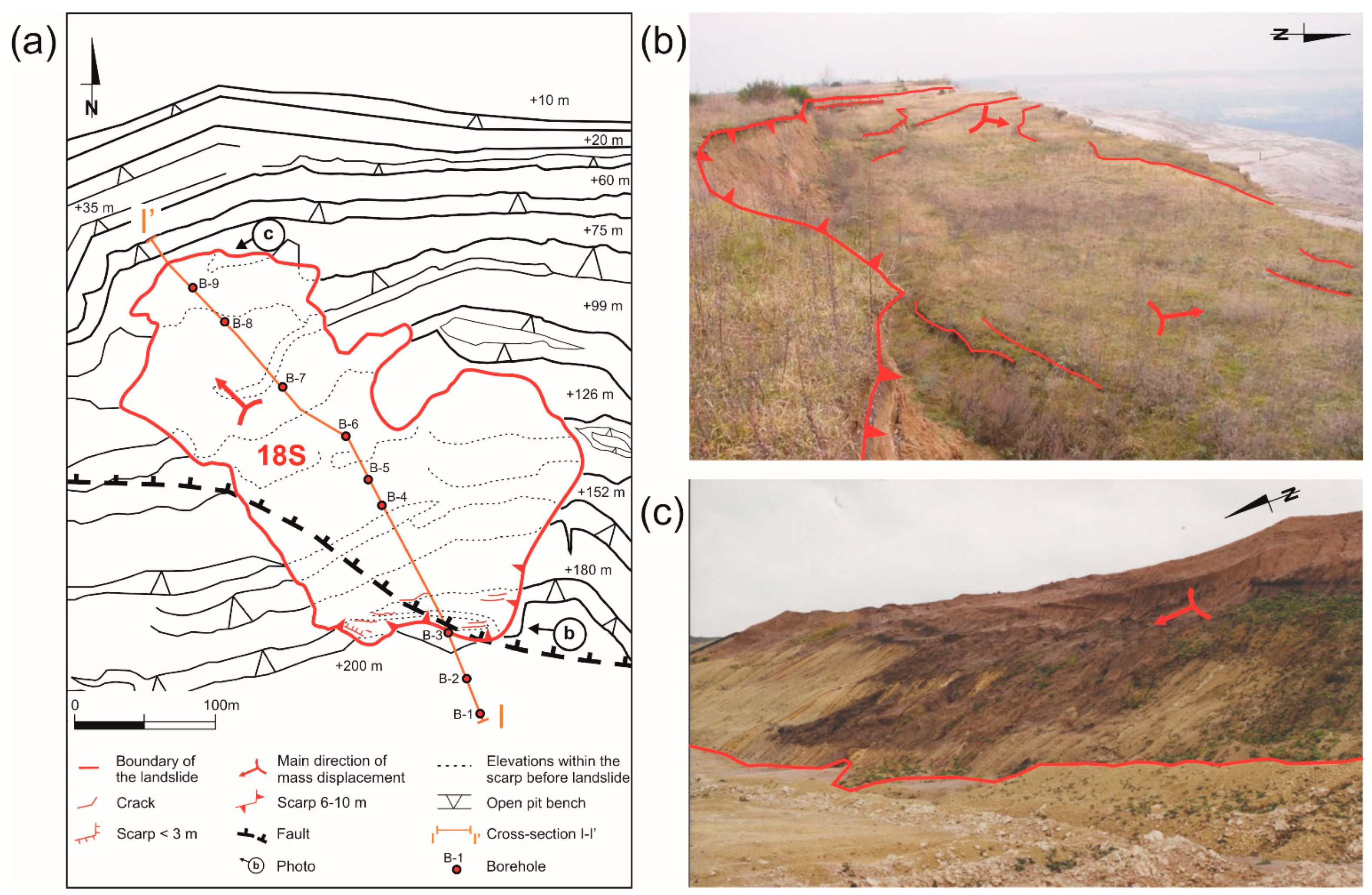
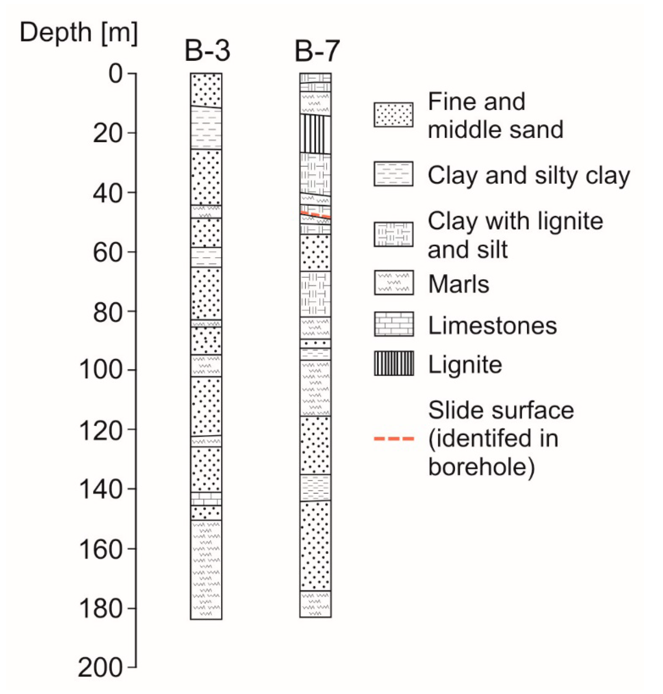
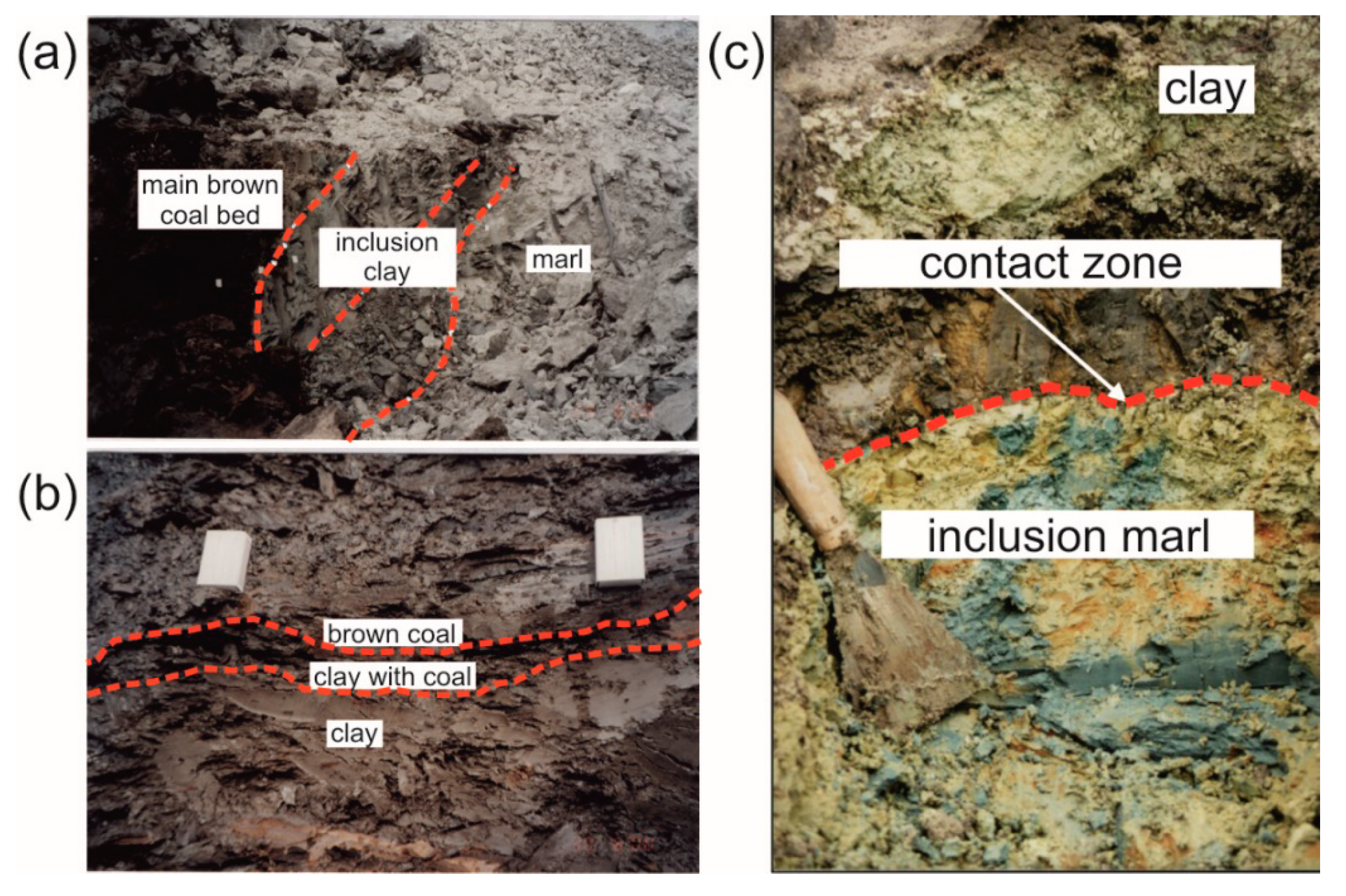
3.1. Site Investigation
- σT—tensile strength,
- σC—compressive strength.
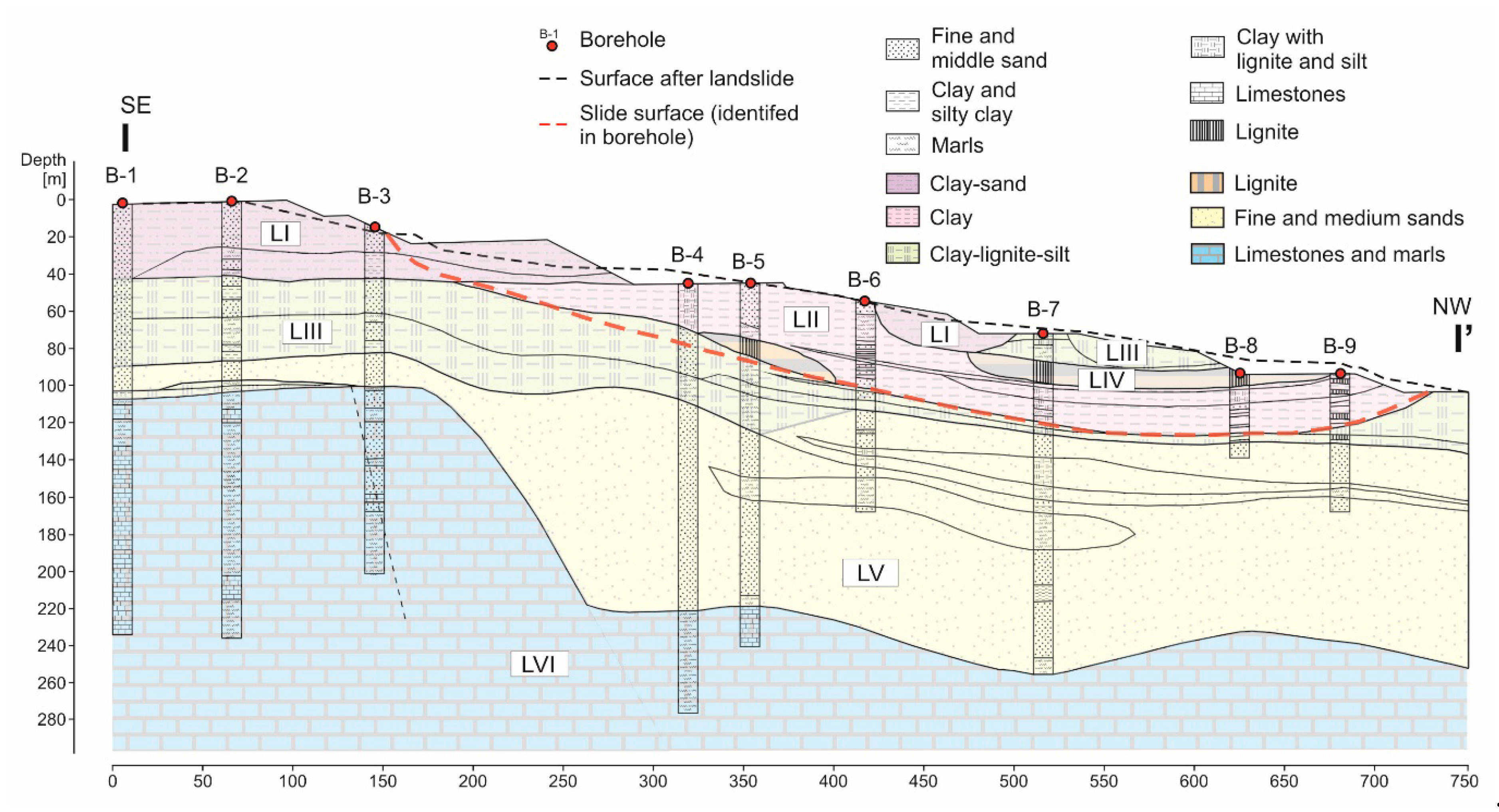
- LI—a clay and sand formation consisting of various-grained, brown-beige quartz sands and clay. In the top part of the formation, there are variegated clay and silt sediments with a sand interbed;
- LII—clay formation with lignite lenses;
- LIII—a clay, lignite, and silt formation consisting of the main layer of lignite A, black, carbonised clays, and silts. In the lower part of the formation, there are light-grey silt and sandy loams;
- LIV—a formation consisting of a multi-layer lignite seam separated by clay and silt;
- LV—a formation consisting of fine and medium sands with inserts of sandy silt, silted sands and silt;
- LVI—Mesozoic bedrock formation consisting of limestones and marls at a depth of approx. 90 to 190 m.
3.2. Sensitivity Analysis
- Selection of input parameters;
- Calculation of sensitivity ratio based on numerical calculations;
- Determination of the most influential parameters based on the quantity of the normalized sensitivity ratio.
- N—number of the most influential parameters (N = 12),
- n—number of sources of information about parameters (n = 2).
3.3. Numerical Stability Analysis
- Selection of sets of input parameters;
- Numerical calculations.
3.4. Probability Analysis
- Development of a P-box graph of the lower and upper limits of the cumulative probability;
- Verification of the calculation results.
- FoS values for each of the source combinations were sorted in ascending order;
- The FoS values within the variability range were rejected, and the minimum and maximum values were adopted for further calculations;
- Each FOS value was assigned a probability of occurrence;
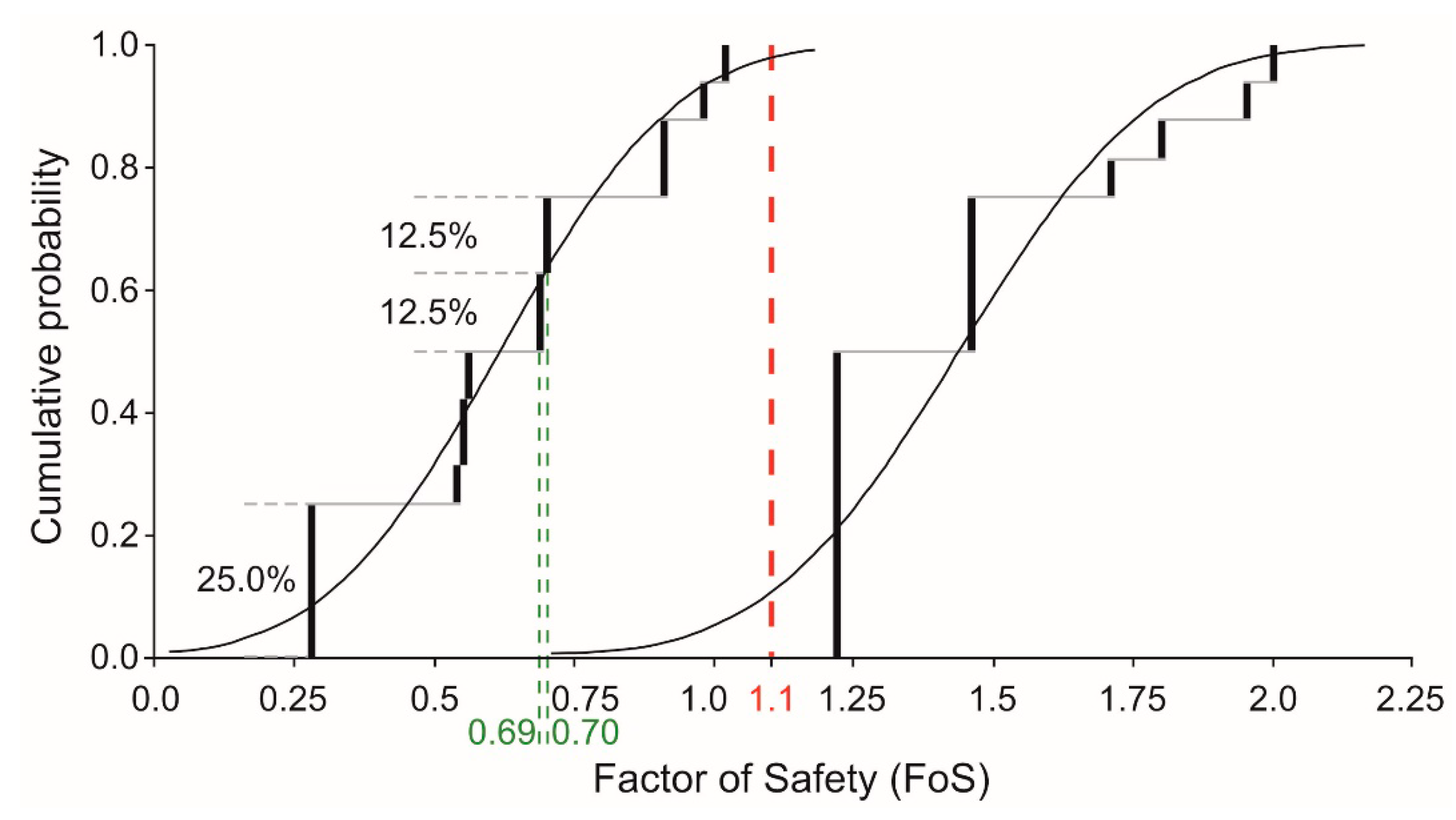
- P-box graphs of FoS values on the horizontal axis were constructed along with the assigned probabilities on the vertical axis. As a result, the upper and lower bounds of the cumulative probability of FoS occurrence were obtained, approximated by the continuous normal distribution function.
4. Results and Discussion
4.1. Sensitivity Analysis
4.2. Numerical Analysis
4.3. Probability Analysis
4.4. Setting the Critical Strength Parameters
5. Conclusions
- The methodology of calculations allowed determination of the slide surface with a factor of safety, most closely to the slide surface identified in boreholes and field observations. In the considered model of the landslide, the slide plane of the landslide developed in lithological units of a complex structure and properties with strongly variable values of strength parameters.
- Numerical calculations using the random set method allowed determination of the set of the most influential input parameters for assessing the stability of the open-pit slope model. The strength parameters of units II and III, particularly the residual cohesion values, had the greatest impact on landslide formation.
- The stability analysis, using the shear strength reduction method and the random set method provided information about different courses of the slide surfaces with the assigned probability of the factor of safety.
- The knowledge of the input critical parameter values was important in further analyses for the following purposes: (a) to increase safety for planning slopes of an open-pit mine; (b) to calculate the stability of other slopes in a given open pit; and (c) for numerical simulations of various types of variants of slope protection.
Author Contributions
Funding
Institutional Review Board Statement
Informed Consent Statement
Data Availability Statement
Acknowledgments
Conflicts of Interest
References
- Singh, V.K.; Prasad, M.; Singh, S.K.; Rao, D.G.; Singh, U.K. Slope design based on geotechnical study and numerical modelling of a deep open-pit mine in India. Int. J. Surf. Min. Reclam. 1995, 9, 105–111. [Google Scholar] [CrossRef]
- Board, M.; Chacon, E.; Varona, P.; Loring, L. Comparative analysis of toppling behaviour at Chuquicamata open-pit mine, Chile. Trans. Inst. Min. Metall. 1996, 105, 1–21. [Google Scholar]
- Hencher, S.R.; Liao, Q.H.; Monaghan, B.G. Modelling slope behaviour for open-pits. Trans. Inst. Min. Metall. 1996, 105, 37–47. [Google Scholar]
- Stacey, T.R.; Xianbin, Y.; Armstrong, R.; Keyter, G.J. New slope stability considerations for deep open-pit mines. J. S. Afr. Inst. Min. Metall. 2003, 103, 373–389. [Google Scholar]
- Yang, X.; Vanapalli, S. Slope Stability Analyses of Outang Landslide Based on the Peak and Residual Shear Strength Behavior. Adv. Eng. Sci. 2019, 51, 55–68. [Google Scholar]
- Bednarczyk, Z. Slope stability analysis for the design of a new lignite open-pit mine. Procedia Eng. 2017, 191, 51–58. [Google Scholar] [CrossRef]
- Franz, J. An Investigation of Combined Failure Mechanisms in Large Scale Open Pit Slopes. Ph.D. Thesis, University of New South Wales, Sydney, Australia, 2009. [Google Scholar]
- Norm EN 1997-1. 2004: Eurocode 7: Geotechnical Design-Part 1: General rules. The European Union per Regulation 305/2011, Directive 98/34/EC, Directive2004/18/EC; Norm EN 1997-1: London, UK, 2004. [Google Scholar]
- Kamai, T. Monitoring the process of ground failure in repeated landslides and associated stability assessments. Eng. Geol. 1998, 50, 71–84. [Google Scholar] [CrossRef]
- Choo, J.; Sohail, A.; Fei, F.; Wong, T. Shear fracture energies of stiff clays and shales. Acta Geotech. 2021, 16, 2291–2299. [Google Scholar] [CrossRef]
- Skempton, A.W. Residual strength of clays in landslides, folded strata and the laboratory. Geotechnique 1985, 35, 3–18. [Google Scholar] [CrossRef]
- Skempton, A.W. Long-term stability of clay slopes. Geotechnique 1964, 14, 77–102. [Google Scholar] [CrossRef] [Green Version]
- Romero, E.; Vaunat, J.; Merchan, V. Suction effects on the residual shear strength of clays. J. Geo-Eng. Sci. 2014, 2, 17–37. [Google Scholar] [CrossRef]
- Souza, M.F.; Nelson, M.G. A Comparison of the Shear Strength Reduction Technique and Limit Equilibrium Method for Slope Stability. In Proceedings of the 52nd US Rock Mechanics/Geomechanics Symposium, Seattle, WA, USA, 17–20 June 2018. [Google Scholar]
- Ural, S.; Yuksel, F. Geotechnical characterization of lignite-bearing horizons in the Afsin-Elbistan lignite basin, SE Turkey. Eng. Geol. 2004, 75, 129–146. [Google Scholar] [CrossRef]
- Soren, K.; Budi, G.; Sen, P. Stability analysis of open pit slope by finite difference method. Int. J. Res. Eng. Technol. 2014, 3, 326–334. [Google Scholar]
- Tao, Z.; Li, M.; Zhu, C.; He, M.; Zheng, X.; Yu, S. Analysis of the critical safety thickness for pretreatment of mined-out areas underlying the final slopes of open-pit mines and the effects of treatment. Shock. Vib. 2018, 2018, 1–8. [Google Scholar] [CrossRef] [Green Version]
- Fang, N.; Ji, C.; Crusoe, G.E., Jr. Stability analysis of the sliding process of the west slope in Buzhaoba Open-Pit Mine. Int. J. Min. Sci. Technol. 2016, 26, 869–875. [Google Scholar] [CrossRef]
- Matheron, G. Random Sets and Integral Geometry; Wiley: New York, NY, USA, 1975. [Google Scholar]
- Nguyen, H.T. On random sets and belief functions. J. Math. Anal. Appl. 2008, 65, 531–542. [Google Scholar] [CrossRef] [Green Version]
- Nasekhian, A.; Schweiger, H.F. Random set finite element method application to tunnelling. In Proceedings of the 4th International Workshop on Reliable Engineering Computing (REC2010), Robust Design—Coping with Hazards, Risk and Uncertainty; Beer, M., Muhanna, R.L., Mullen, R.L., Eds.; Research Publishing: Singapore, 2010; pp. 369–385. [Google Scholar]
- Hall, J.W.; Rubio, E.; Anderson, M.J. Random sets of probability measures in slope hydrology and stability analysis. ZAMM J. Appl. Math. Mech. 2004, 84, 710–720. [Google Scholar] [CrossRef]
- Schweiger, H.F.; Peschl, G.M. Reliability analysis in geotechnics with the random set finite element method. Comput. Geotech. 2005, 32, 422–435. [Google Scholar] [CrossRef]
- Pilecki, Z.; Stanisz, J.; Krawiec, K.; Woźniak, H.; Pilecka, E. Numerical stability analysis of slope with use of random set theory. Zesz. Nauk. IGSMiE PAN 2014, 86, 5–17. (In Polish) [Google Scholar]
- FLAC v. 7.0., Factor of Safety; Itasca Consulting Group: Minneapolis, MN, USA, 2011.
- Cullen, R.M.; Donald, I.B. Residual strength determination in direct shear. In Proceedings of the 1st Australia-New Zealand Conference on Geomechanics, Melbourne, Australia, 9–13 August 1971; Volume 1, pp. 1–10. [Google Scholar]
- Akis, E.; Mekael, A.; Yilmaz, M.T. Investigation of the effect of shearing rate on residual strength of high plastic clay. Arab. J. Geosci. 2020, 13, 66. [Google Scholar] [CrossRef]
- Kaczmarczyk, R.; Rybicki, S. Powierzchnie strukturalne w górotworze złóż węgla brunatnego, ich charakterystyka i właściwości fizykomechaniczne [Structural surfaces in the lignite seams, their characteristics, and physicomechanical properties]. Górnictwo Geoinżynieria 2007, 31, 237–245. (In Polish) [Google Scholar]
- Norm PN-B-04481:1988. Grunty Budowlane. Badania Próbek Gruntu [Building Soil. Soil Samples Testing]; Norm PN-B-04481: Warsaw, Poland, 1988. (In Polish) [Google Scholar]
- Norm PN-G-04303:1997. Skały Zwięzłe—Oznaczenie Wytrzymałości na Ściskanie z Użyciem Próbek Foremnych [Determination of Compressive Strength with the Use of Regular Samples]; Norm PN-G-04303: Warsaw, Poland, 1997. (In Polish) [Google Scholar]
- Peschl, G.M. Reliability Analysis in Geotechnics with the Random Set Finite Element Method. Ph.D. Thesis, Graz University of Technology, Graz, Austria, 2004. [Google Scholar]
- Momeni, E.; Poormoosavian, M.; Mahdiyar, A.; Fakher, A. Evaluating random set technique for reliability analysis of deep urban excavation using Monte Carlo simulation. Comput. Geotech. 2018, 100, 203–215. [Google Scholar] [CrossRef]
- Tonon, F.; Bernardi, A.; Mammio, A. Determination of parameters in rock engineering by means of Random Set Theory. Reliab. Eng. Syst. Saf. 2000, 70, 241–261. [Google Scholar] [CrossRef]
- Sekhavatian, A.; Choobbasti, A.J. Application of random set method in a deep excavation: Based on a case study in Teheran cemented alluvium. Front. Struct. Civ. Eng. 2018, 13, 66–80. [Google Scholar] [CrossRef]
- Shen, H.; Abbas, S.M. Rock slope reliability analysis based on distinct element method and random set theory. Int. J. Rock Mech. Min. Sci. 2013, 61, 15–22. [Google Scholar] [CrossRef]


| Lithological Unit | LI | LII | LIII | LIV | LV | LVI | |||
|---|---|---|---|---|---|---|---|---|---|
| Grain-size distribution (%) | Clay | min | 21.0 | 38.0 | 12.0 | – | 69.0 | – | |
| max | 25.0 | 49.0 | 50.0 | – | 71.0 | – | |||
| mean | 23.2 | 42.6 | 31.0 | – | 70.4 | – | |||
| Silt | min | 52.0 | 40.0 | 44.0 | – | 16.0 | – | ||
| max | 56.0 | 44.0 | 61.0 | – | 22.0 | – | |||
| mean | 24.0 | 42.2 | 52.5 | – | 19.0 | – | |||
| Sand | min | 21.0 | 7.0 | 5.0 | – | 9.0 | – | ||
| max | 24.0 | 22.0 | 26.0 | – | 12.0 | – | |||
| mean | 22.7 | 15.2 | 15.2 | – | 11.0 | – | |||
| Gravel | min | 0.0 | 0.0 | 0.0 | – | 0.0 | – | ||
| max | 0.0 | 0.0 | 3.0 | – | 0.0 | – | |||
| mean | 0.0 | 0.0 | 1.2 | – | 0.0 | – | |||
| Moisture content (%) | min | 29.1 | 25.6 | 19.7 | 29.6 | 19.3 | 11.1 | ||
| max | 47.5 | 64.2 | 46.8 | 82.5 | 31.8 | 12.8 | |||
| mean | 42.5 | 46.6 | 28.1 | 62.5 | 24.9 | 12.3 | |||
| Atterberg limits | Plastic limit (%) | min | 26.6 | 26.1 | 22.2 | 33.8 | 20.8 | 17.7 | |
| max | 29.7 | 50.8 | 42.6 | 104.5 | 37.2 | 18.9 | |||
| mean | 27.6 | 42.5 | 33.2 | 70.3 | 28.7 | 18.5 | |||
| Liquid limit (%) | min | 81.2 | 61.9 | 40.4 | 56.5 | 41.8 | 21.2 | ||
| max | 87.1 | 110.5 | 93.1 | 157.8 | 140.6 | 22.5 | |||
| mean | 84.6 | 99.5 | 72.4 | 115.5 | 82.3 | 21.5 | |||
| Plasticity index (–) | min | 54.3 | 35.8 | 17.9 | 21.2 | 19.9 | 2.4 | ||
| max | 60.4 | 66.6 | 94.1 | 64.2 | 94.1 | 3.8 | |||
| mean | 57.1 | 57.0 | 38.3 | 45.5 | 63.6 | 3.0 | |||
| Liquidity index (–) | min | 0.01 | −0.14 | −0.28 | −0.34 | −0.15 | −1.5 | ||
| max | 0.35 | 0.32 | 0.11 | −0.11 | −0.05 | −2.7 | |||
| mean | 0.26 | 0.0 | −0.1 | −0.17 | −0.07 | −2.1 | |||
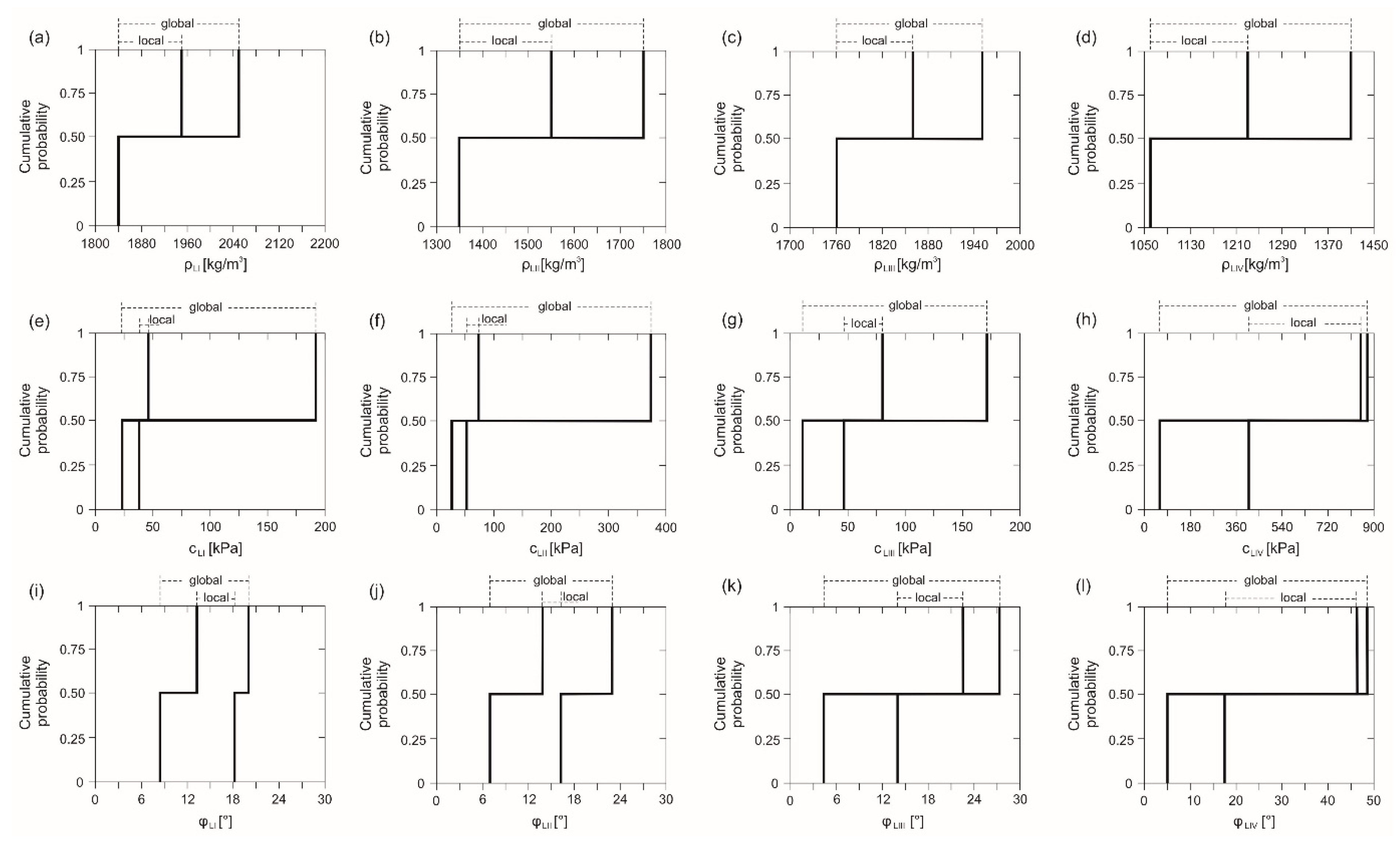
| Bulk density (kg/m3) | Peak | min | 1840 | 1350 | 1760 | 1060 | 1850 | 2540 | |
| max | 2050 | 1750 | 1950 | 1410 | 2640 | ||||
| mean | 1945 | 1550 | 1855 | 1235 | 2590 | ||||
| Residual | min | 1840 | 1350 | 1760 | 1060 | – | |||
| max | 1950 | 1550 | 1860 | 1230 | – | ||||
| mean | 1895 | 1450 | 1810 | 1145 | – | ||||
| Cohesion (kPa) | Peak | min | 47.0 | 52.0 | 46.0 | 850.0 | 0.0 | 5500.0 | |
| max | 191.0 | 374.0 | 172.0 | 870.0 | 12,800.0 | ||||
| mean | 119.0 | 213.0 | 109.0 | 860.0 | 9150.0 | ||||
| Residual | min | 24.6 | 27.5 | 10.3 | 68.0 | – | |||
| max | 37.5 | 73.5 | 78.0 | 420.0 | – | ||||
| mean | 31.1 | 50.5 | 44.2 | 244.0 | – | ||||
| Internal friction angle (°) | Peak | min | 13.5 | 14.0 | 14.0 | 46.0 | 32.0 | 11.5 | |
| max | 21.2 | 25.2 | 27.3 | 48.0 | 41.8 | ||||
| mean | 17.4 | 19.6 | 20.7 | 47.0 | 26.7 | ||||
| Residual | min | 13.5 | 12.9 | 4.0 | 5.0 | – | |||
| max | 15.6 | 31.3 | 22.8 | 17.0 | – | ||||
| mean | 14.6 | 17.1 | 13.4 | 11.0 | – | ||||
| Unit | Data Source | Bulk Density (kg/m3) | Cohesion (kPa) | Internal Friction Angle (°) | ||||||
|---|---|---|---|---|---|---|---|---|---|---|
| Min | Max | Mean | Min | Max | Mean | Min | Max | Mean | ||
| LI | A: peak | 1840 | 2050 | 1945 | 47.0 | 191.0 | 119.0 | 13.4 | 18.2 | 15.8 |
| B: resid. | 1840 | 1950 | 1895 | 24.6 | 37.5 | 31.1 | 8.6 | 20.0 | 14.3 | |
| LII | A: peak | 1350 | 1750 | 1550 | 52.0 | 374.0 | 213.0 | 14.0 | 16.1 | 15.1 |
| B: resid. | 1350 | 1550 | 1450 | 27.5 | 73.5 | 50.5 | 7.0 | 23.3 | 15.2 | |
| LIII | A: peak | 1760 | 1950 | 1855 | 46.0 | 172.0 | 109.0 | 14.0 | 27.3 | 20.7 |
| B: resid. | 1760 | 1860 | 1810 | 10.3 | 78.0 | 44.2 | 4.0 | 22.8 | 13.4 | |
| LIV | A: peak | 1060 | 1410 | 1235 | 850.0 | 870.0 | 860.0 | 46.0 | 48.0 | 47.0 |
| B: resid. | 1060 | 1230 | 1145 | 68.0 | 420.0 | 244.0 | 5.0 | 17.0 | 11.0 | |
| LV | – | – | – | 1850 | – | – | 0.0 | – | – | 32.0 |
| LVI | – | – | – | 2590 | – | – | 9150 | – | – | 26.7 |
| Combination Number | Combinations of the Most Influential Parameters from Different Sources A and B | |||
|---|---|---|---|---|
| 1 | cLI (A) | cLII (A) | cLIII (A) | φLIII (A) |
| 2 | cLI (A) | cLII (A) | cLIII (A) | φLIII (B) |
| 3 | cLI (A) | cLII (A) | cLIII (B) | φLIII (A) |
| 4 | cLI (A) | cLII (A) | cLIII (B) | φLIII (B) |
| 5 | cLI (A) | cLII (B) | cLIII (A) | φLIII (A) |
| 6 | cLI (A) | cLII (B) | cLIII (A) | φLIII (B) |
| 7 | cLI (A) | cLII (B) | cLIII (B) | φLIII (A) |
| 8 | cLI (A) | cLII (B) | cLIII (B) | φLIII (B) |
| 9 | cLI (B) | cLII (A) | cLIII (A) | φLIII (A) |
| 10 | cLI (B) | cLII (A) | cLIII (A) | φLIII (B) |
| 11 | cLI (B) | cLII (A) | cLIII (B) | φLIII (A) |
| 12 | cLI (B) | cLII (A) | cLIII (B) | φLIII (B) |
| 13 | cLI (B) | cLII (B) | cLIII (A) | φLIII (A) |
| 14 | cLI (B) | cLII (B) | cLIII (A) | φLIII (B) |
| 15 | cLI (B) | cLII (B) | cLIII (B) | φLIII (A) |
| 16 | cLI (B) | cLII (B) | cLIII (B) | φLIII (B) |
| Factor of Safety | Lower Limit | Upper Limit |
|---|---|---|
| Distribution | Normal | Normal |
| Mean value | 0.62 | 1.44 |
| Standard deviation | 0.25 | 0.27 |
| Probability of the FoS = 1.1 | 0.97 | 0.10 |
| The Most Influential Parameter | Number of the Set of Input Parameters | ||||
|---|---|---|---|---|---|
| 105 | 161 | 169 | 225 | 233 | |
| cLI (kPa) | 24.6 | 24.6 | 37.5 | 24.6 | 37.5 |
| cLII (kPa) | 27.5 | 52.0 | 52.0 | 27.5 | 27.5 |
| cLIII (kPa) | 10.3 | 10.3 | 10.3 | 10.3 | 10.3 |
| φLIII (kPa) | 14.0 | 14.0 | 14.0 | 14.0 | 14.0 |
| FoS | 0.703 | 0.701 | 0.702 | 0.694 | 0.692 |
| Lithological Unit | Bulk Density (kg/m3) | Cohesion (kPa) | Internal Friction Angle (°) |
|---|---|---|---|
| LI | 1950 | 24.6 | 14.3 |
| LII | 1550 | 27.5 | 15.2 |
| LIII | 1860 | 10.3 | 14.0 |
| LIV | 1230 | 469.0 | 26.5 |
| LV | 1850 | 0.0 | 32.0 |
| LVI | 2590 | 9150.0 | 26.7 |
Publisher’s Note: MDPI stays neutral with regard to jurisdictional claims in published maps and institutional affiliations. |
© 2021 by the authors. Licensee MDPI, Basel, Switzerland. This article is an open access article distributed under the terms and conditions of the Creative Commons Attribution (CC BY) license (https://creativecommons.org/licenses/by/4.0/).
Share and Cite
Pilecka, E.; Stanisz, J.; Kaczmarczyk, R.; Gruchot, A. The Setting of Strength Parameters in Stability Analysis of Open-Pit Slope Using the Random Set Method in the Bełchatów Lignite Mine, Central Poland. Energies 2021, 14, 4609. https://doi.org/10.3390/en14154609
Pilecka E, Stanisz J, Kaczmarczyk R, Gruchot A. The Setting of Strength Parameters in Stability Analysis of Open-Pit Slope Using the Random Set Method in the Bełchatów Lignite Mine, Central Poland. Energies. 2021; 14(15):4609. https://doi.org/10.3390/en14154609
Chicago/Turabian StylePilecka, Elżbieta, Jacek Stanisz, Robert Kaczmarczyk, and Andrzej Gruchot. 2021. "The Setting of Strength Parameters in Stability Analysis of Open-Pit Slope Using the Random Set Method in the Bełchatów Lignite Mine, Central Poland" Energies 14, no. 15: 4609. https://doi.org/10.3390/en14154609