Nexus between Financial Development, Renewable Energy Consumption, Technological Innovations and CO₂ Emissions: The Case of India

Abstract

Concerns regarding environmental sustainability have generally been an important element in achieving long-term development objectives. However, developing countries struggle to deal with these concerns, which all require specific treatment. As a result, this study explores the interaction between financial development, renewable energy consumption, technological innovations, and CO₂ emissions in India from 1980 to 2019, taking into account the critical role of economic progress and urbanization. The Autoregressive Distributed Lag (ARDL) model is used to quantify long-run dynamics, while the Vector Error Correction Model is used to identify causal direction (VECM). According to the study’s conclusions, financial development has a considerable positive impact on CO₂ emissions. The coefficient of renewable energy consumption and technical innovations, on the other hand, is strongly negative in both the short and long run, indicating that increasing these measures will reduce CO₂ emissions. Furthermore, economic expansion and urbanization have a negative impact on environmental quality since they emit a significant amount of CO₂ into the atmosphere. The results of the robustness checks were obtained using the Fully Modified Ordinary Least Squares (FMOLS), the Dynamic Ordinary Least Squares (DOLS), and the Canonical Cointegration Regression (CCR) approaches to verify the findings. The VECM results reveal that there is long-run causality in CO₂ emissions, financial development, renewable energy utilization, and urbanization. A range of diagnostic tests were also used to confirm the validity and reliability. This study delivers new findings that contribute to the existing literature and may be of particular interest to the country’s policymakers in light of the financial system and its role in environmental issues.

1. Introduction

Energy is a necessary component for an economy to adopt long term progress. Its ever-increasing need has intensified in recent times and is still increasing currently. The increased demand for energy is due to a number of factors including population increase, improved lifestyles, manufacturing advancements, and economic competitiveness. Therefore, global energy consumption surged by 44 percent between 1971 and 2014 [1,2]. Unnecessary burning of fossil fuels releases massive amounts of carbon dioxide (CO₂) emissions into the air, causing negative environmental impacts such as climate change. CO₂ emissions have grown by 31% during the last 200 years, and the average global warming has risen by 0.4–0.8 °C in the past century [3]. In recent years, environmental pollution, primarily triggered by CO₂ emissions, has become a worldwide problem. Governments have recently been more cognizant of the concern; for example, the Kyoto Protocol entered into effect in 2005 to decrease overall emissions of greenhouse gases created by industrialized nations. Moreover, the European Union (EU) Commission funds many research initiatives aimed at reducing fossil fuel usage, improving energy efficiency, and developing new technological advances, especially for renewable energy [4].

Apart from environmental problems, importing economies face the threat of energy uncertainty due to their reliance on fossil fuel usage on a large scale. As of 2017, oil was the largest widely utilized resource on the planet, accounting for one-third of global energy use. The Organization of Petroleum Exporting Countries (OPEC) controls 71.5 percent of overall oil reserves, whereas the rest depend primarily on producing nations [5]. Long-term energy policy is crucial for sustainable projects to ensure energy supply in sync with economic success and progress. In the short term, energy stability necessitates the continuous supply of the desired source of energy as well as constant costs to make it more affordable [6]. The fairly unstable character of fossil fuel markets, on the other hand, puts importing nations in danger of energy instability. The disturbance of the energy supply–demand equilibrium is predicted to have serious economic impacts. As a result, energy-based countries are subject to conservation regulations that restrict energy usage [7,8].

Renewable energy has the ability to be a useful instrument in achieving energy diversity. Less reliance on fossil energy supplies indicates greater resilience to energy market disruptions. Furthermore, renewable energy generation has the potential to avoid additional environmental harm. Transferring from fossil-fuel-based energy to green energy generation, on the other hand, can be difficult. The expense of implementing renewable energy is one of the most significant challenges. When opposed to fossil fuel-based energy expenditures, there are a variety of financial challenges to address, including greater infrastructure, operational expenses, and start-up costs. In this context, the financial sector plays a crucial role in running an economic system by generating funds and contributing to transparent dealings and management of capital. A secure financial system is crucial for the smooth transfer of resources and makes business operations more efficient, which results in stronger economic progress [9,10]. According to Yu and Qayyum [11], the financial sector plays a significant role in promoting economic evolution and affects environmental efficiency. A developed financial system contributes to stimulating the economy, and economies with an effective financial system are expected to have a good atmosphere. A strong financial market enables businesses to implement innovative and energy-efficient technology that lowers pollution. Likewise, scaling up renewable energy funding will be critical in India, as fulfilling these commitments will necessitate an investment of nearly USD 189 billion by 2022. Nevertheless, according to the Climate Policy Initiative (CPI), real realized contribution may fall short of the criteria by 29 percent (USD 17 billion) for equity and 27 percent (USD 36 billion) for debt [12]. To reduce the financial vacuum and grow the renewable energy sector, India has implemented a number of institutional reforms at both the state and federal levels. The federal government has provided rapid depreciation, generation-based subsidies, and viability gap financing, while state-level policy assistance has often taken the shape of feed-in tariffs, net metering, and tax/duty concessions [13]. Notwithstanding these encouraging federal and state regulations, financial issues are unavoidable given the overreliance on commercial banks for credit funding. Generally, Indian renewables initiatives have greater financing expenses than corresponding initiatives in the United States or Europe, which is a significant barrier to their adoption due to the high initial cost. Given the high renewable energy goals but minimal government resources, policymakers must consider the cost-effectiveness of supporting initiatives.

In contrast, Tamazian et al. [14] stated that an established finance system stimulates economic development, triggering more emissions and severe harm to the environment. A stable financial system can finance the business operations to improve output and helps companies in their production by offering loans at a reduced interest rate that induces more power usage and increases carbon emissions [9,15]. The impact of financial development on the ecosystem [16,17] has become a hot topic; the present study, therefore, adds financial development into energy-growth-environmental links and looks at its importance in India for sustained growth. Therefore, the research aims at examining the impacts of Indian financial development, the consumption of renewable energy, technological innovation, and economic development on CO₂ emissions. India has been selected because its economy is heavily reliant on the financial sector, which has been one of the largest developing sectors in the economy. India’s financial system focuses mostly on commercial banks, non-banking financial institutions, rural banks, pensions, mutual funds, and insurance companies [18]. Since the 2011 Financial Sector Assessment Program (FSAP) (For more details visit: https://www.imf.org/~/media/Files/Publications/CR/2017/cr17390.ashx (assessed on 20 August 2020)), India has experienced rapid expansion both in economic growth and financial instruments, backed by major structural reforms and progress in the balance of trade. Increased diversification, business focus, and technology-driven integration, accompanied by appropriate governance, legislative, and disciplinary mechanisms, have benefited financial industry development. However, the financial system is beset by difficulties, and economic growth has gradually decelerated. High nonperforming assets (NPAs) and the slow deflation and reconstruction of corporate balance sheets are putting the financial system’s stability to the test and restricting financing and development. No empirical research on the effect of financial development on CO₂ emissions in India was conducted to the best of our knowledge, while taking account of the crucial role of renewable energy consumption, technological innovation and economic development. The connection between financial development and CO₂ emissions is an important issue for Indian policymakers. The latest time-series data is used for econometric investigation along with the most suitable econometric approach for time series, i.e., the Autoregressive Distributed Lag (ARDL) model, and then checking the causal associations between variables through the Vector Error Correction Model (VECM) Granger causality method. In addition, this study also employs fully modified ordinary least squares (FMOLS), dynamic ordinary least squares (DOLS), and canonical cointegration regression (CCR) techniques to investigate the robustness of the outcomes. Based on the results, significant policy repercussions for the government and policymakers are proposed.

The rest of the research is as follows. Section 2 covers the review of the related literature. Section 3 covers the econometric methodology and data source. The findings, interpretation, and discussion are presented in Section 4. Section 5 summarizes the research with policy suggestions.

2. Literature Review

This study examines the effect of financial development (FD), renewable energy consumption (REC), and technological innovation (TI) on CO₂ emissions in India. The study divides the literary review into three parts: one describes the links between the FD and CO₂ emissions, while the second and third parts discuss the REC and CO₂ emissions, and the TI and CO₂ emissions.

Recently, many financial development variables were incorporated into the environment-growth-energy model, for instance, [19,20]. According to the above-mentioned investigators, in the discussion on the relationship between environmental factors, economic development, and energy use, the attempts to include the measures of financial development are not unreal. It can lead to foreign direct investment (FDI), expertise and research, and innovation, all of which can lower energy consumption and boost economic development [21]. As a result, environmental quality will increase. Saud et al. [22] studied the impact of CO₂ emissions in 59 BRI economies from 1980 to 2016 on FD, economic development, energy consumption, and international trade. They argue that increased energy usage and economic expansion lead to environmental deterioration, whereas increased trade openness and financial advancement reduce environmental impacts by reducing pollution. Likewise, Zafar et al. [23] discussed the impact of FD and globalization on carbon emissions in the OECD economies and concluded that FD and globalization, through a reduction in pollution, greatly improve environmental performance. In six South Mediterranean countries (SMCs), Kahouli [24] uncovered the link between growth-energy-financial development between 1995 and 2015. He revealed the long-standing cointegration of variables and suggested that the key element for improving energy utilization was FD. In contrast, some researchers contend that FD made a demand for energy, which had a negative impact on the atmosphere due to increased carbon emissions. Guo et al. [25] used provincial data from China from 1997 to 2015 to probe the effect of FD on carbon emissions. They concluded that the intensity of trading stocks and the reliability of FD increased the level of carbon emissions. Also, the relations between FD, international trade, and the environmental performance of Iran were investigated by Esmaeilpour Moghadam and Dehbashi [26]. According to their findings, FD accelerated environmental pollution.

As an environmentally friendly option to non-renewable energy, such as coal, gasoline, and oil, renewable energy sources such as wind, hydro, sun, and many more have grown in popularity. Evidently, these sources of energy have the possibility to provide levels of non-carbon clean energy relatively close to the levels previously provided by carbon-based energy, while continuously lowering greenhouse gas levels in the atmosphere. Several studies were carried out over the last few years, utilizing various time frames, regions, techniques, and parameters to determine how and to what degree REC can reduce CO₂ emissions. For example, from the years 1980 to 2012, Zoundi [27] scrutinized the connection between CO₂ emissions and the REC in 25 African economies. It was stated by Cherni and Essaber Jouini [28] that REC decreased CO₂ emissions due to economic development, whereas fossil fuels boosted CO₂ emissions in Tunisia. Waheed et al. [29] examined the link between the use of the REC, the use of agriculture in forests, and emissions of CO₂ in Pakistan from 1990 to 2014. Chen et al. [30] investigated the link between economic development, REC and non-REC, and CO₂ emissions in China from 1995 to 2012. Aside from failing to verify the Kuznets curve hypothesis, the researchers concluded contradictory findings regarding the effect of REC and CO₂ emissions across various Chinese areas. In the same year, Chen et al. [31] analyzed the association between CO₂ emissions, economic progress, REC and non-REC, and international trade in China from 1980 to 2014. This research found that the Kuznets curve supported and discovered a negative correlation between REC and CO₂ emissions in terms of empirical results. Charfeddine and Kahia [32] studied the effect of REC, financial advancement, and economic expansion on CO₂ emissions in the Middle East and North Africa (MENA) from 1980 to 2015, however, the estimation results revealed a minimal effect of REC and financial advancement on CO₂ emissions.

In addition, the impact on pollution reduction is believed to be significant for technological innovations (TI). Technological innovations have decreased CO₂ emissions and enhanced environmental performance in host countries in conjunction with environmental prevention initiatives. Previous studies indicate that the promising influence of TI and CO₂ emissions have received much attention. The majority of academics opt for patents as a measure for TI, see, for example, [33,34] because they protect intellectual property and business rights that contribute to solving environmental challenges by developing technology [35]. According to Yu and Du [36], impartial innovation initiatives have played an important role in China’s CO₂ emissions mitigation. According to Brandão Santana et al. [37], TI has aided the advancement of a reliable energy sector while also allowing for long-term economic growth across the BRICS and G7 countries. Similarly, from 1971 to 2013 in Malaysia, Yii and Geetha [38] found a link between technological innovation, growth, use of power, energy prices, and CO₂ emissions. It was shown, in the absence of a long-term association, that technological innovation resulted in a short-term reduction in CO₂ emissions. The effect of TI on the energy sector on CO₂ emissions in China was studied by Jin, Duan, Shi, and Ju [39]. The empirical results indicate that TI improves energy efficiency in the energy sector and therefore decreases CO₂ emissions. As a result, the administration must spend on energy research to secure minimal pollution. Similarly, Aldieri et al. [40] agreed that innovation contributes significantly to lower CO₂ emissions in OECD economies. Su and Moaniba [41], on the other hand, argue that the inconsistent findings and empirical proof demonstrating the insignificant influence of TI and/or climate-related innovations on CO₂ emissions must be acknowledged. Raiser et al. [34] noted that patents aim to limit progress and are seen as a barrier in remediation of climate change, in accordance with this insinuation.

3. Econometric Methodology and Data Source

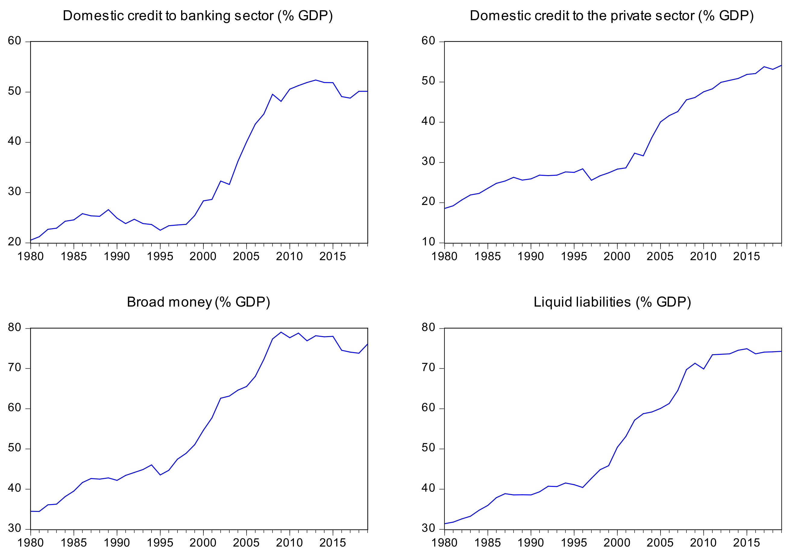
3.1. Data Source

The study sought to examine the dynamic association between the FD index, REC, TI, economic development, urbanization and CO₂ emissions in India by utilizing the ARDL cointegration technique. The data employed in this study ranges from 1980 to 2019. The dependent variable is the emission of CO₂ (metric tons per capita). FD measures as a composite financial development index. REC measures as total energy consumption of renewable energy sources, including hydro, bioenergy, solar, geothermal, wind and ocean energy sources. TI, measured both by the resident and non-resident in patent applications, provides the right to innovate a method or product that guarantees a new approach. Economic development is measured as GDP per capita (constant $2010), and URP is measured as urban population (% total population). The data of CO₂ emission is collected from BP Statistical Review, and the data of all other variables are gathered from the World Bank.

3.2. Composite Financial Development Index

Several parameters have been used to evaluate financial development in the literature. Many researchers, for instance, have used broad money (M2) and liquid liabilities (M3) to assess financial development. However, Jalil and Feridun [42] claim that M2 does not accurately reflect the financial sector progress. They argue that because a major component of M2 is used to monitor currency stability, we would refer to it as monetization rather than financial development. Liquid liabilities, on the other hand, do not fully represent financial advancement because they only represent the volume of the financial industry [43]. Private sector domestic credit (including credit, non-equity securities purchases, accounts receivables, and commercial loans) is also used as a financial development measure [44], although Shahbaz et al. [45] provide domestic private-sector loans as a useful measure of constructive investment activity. Finding an appropriate measure for financial development that can encompass its entire performance is a fundamental topic in the empirical field of economics [46]. Many investigators utilize the proportion of the financial sector to evaluate financial intermediaries. However, Levine et al. [47] argue that it is a simplistic measure and that private credit is an appropriate surrogate. According to Ang [46], credit to the private sector is a preferable element for measuring financial progress since the private sector makes better choices about how to deploy its resources than the government sector. In the existence of a variety of financial mechanisms that present in many countries, it is necessary for the investigator to develop measurements that can represent their true influence [47].

Depending on the preceding argument and the importance of the financial sector to an economy, the current research constructs a composite index that seeks to capture all aspects of FD. Considering past studies for example, [46,48,49], the present study creates an index for FD using four distinct financial sector predictors: (a) domestic credit to the private sector (percent of GDP), (b) domestic credit to banking sector (percent of GDP), (c) liquid liabilities (M3) (percent of GDP), and (d) broad money (M2) (percent of GDP). Thus, the functional association between the four parameters listed above could be expressed as follows:

FD = f (a, b, c, d)

The variables a, b, c and d are acquired from the World Development Indicator.

These parameters may cause a multicollinearity issue if utilized combined in a regression; therefore, by using a well-known analytical technique known as the principal component analysis (PCA), we create a composite FD index. We could transform a large range of parameters (correlated) into fewer factors (uncorrelated) utilizing this technique without affecting the actual volatility in the dataset [50,51]. We created a composite index for FD employing the following equation and components taken from factor analysis.

$$\mathrm{FD} \mathrm{Index}={{\displaystyle \sum }}_{i=1}^n{w}_i\times F{S}_i$$

where the FD Index is our desired index, FS_i is the corresponding component value of each component (financial indicator), and w_i is the weight (the proportion of variance described by every predictor to variability described by all other indicators), and it is calculated as follows:

$$w_i=\left[\frac{v_i}{{\sum }_{i=1}^n{v}_i}\right]\times 100$$

where w_i indicates the component’s weight as the ratio of variance to the variability as defined by all other factors due to that specific factor (v_i), and n indicates the overall number of factors [52].

Table 1. Principal Component Analysis for Financial Development Index.

Number	Eigenvalue	Proportion	Cumulative
1	3.9168	0.9792	0.9792
2	0.0794	0.0170	0.9991
3	0.0235	0.0038	1.0000
4	0	0.0000	1.0000
Financial Indicators	Factor loadings	Communalities	Factor scores
DCP	0.9924	0.9912	0.3012
DCB	0.9951	0.9971	0.3121
M2	0.8701	0.8505	0.2669
M3	0.9412	0.9334	0.2801

Note: DCP is domestic credit to the private sector, DCB denotes domestic credit to the banking sector, M2 represents broad money, and M3 is liquid liabilities.

displays the results of the PCA. The only component with an eigenvalue higher than one is the first (3.9168). This factor is superior because it covers approximately 97.92% of the standardized variation. As a result, just one component is derived from this investigation. Furthermore, Figure 1 indicates the trends of the elements of the FD index in India during the sample period, respectively. To summarize, the DCB exhibits an increased tendency from 1980 to 2019, despite volatility across various sample periods (1990–1995), and then begins to show an increasing trend for the remainder of the time. Likewise, DCP also shows a rising trend. Similarly, BRM shows a mixed tendency with significant variations during the time, it begins to rise rapidly since 1980–2009, but it starts decreasing from 2010 onwards. Finally, LQL depicts upward trends in India during the studied period.

3.3. Theoretical Rationale and Model Specification

This paper studies the link between the FD index, REC, TI, and CO₂ emissions, while considering the vital role of India’s GDP and URP. It is claimed by Zakaria and Bibi [53] that FD is not only essential for the progress of the economy but also essential for climatic change in the country. They also stated that robust and advanced financial sectors improve environmental performance by strengthening the host country’s research and development (R&D) via FDI, supplying clean technology to enterprises, supplying low-cost credit for environmentally friendly initiatives and technical advancements, and offering benefits to enterprises that follow environmental standards and guidelines. By incorporating REC methods for expansion and energy-efficient technology, REC could have an influence on environmental performance [54,55]. By bringing energy advancements and energy-efficient equipment, technological innovations could have an impact on environmental performance [56,57]. Yang et al. [50] argued that economic progress is a main cause of high CO₂ emissions because the development of an economy relies on high energy consumption, which ultimately affects the performance of the environment. Further, the link between urbanization and environmental quality is influenced by the link between urbanization and economic growth [58]. Based on these claims, we design the specific CO₂ emissions model as following:

CO_2t = f (FD_t, REC_t, TI_t, GDP_t, URP_t)

(1)

where CO_2t, FD_t, REC_t, TI_t, GDP_t, and URP_t are CO₂ emissions, financial development, renewable energy consumption, technological innovations, economic growth, and urban population, respectively. For empirical investigation, we converted all parameters to natural-log to use a log-linear configuration instead of a linear configuration. Shahbaz et al. [59] assert that a log-linear configuration offers much more stable and accurate findings. Similarly, another advantage of the log-linear model is that a log transformation is a simple way to convert a significantly skewed parameter into a more normalized dataset. When estimating variables having non-linear interactions, the likelihood of making errors is skewed negatively. Therefore, following other researchers [48,49,50,51], we also used the log-linear method for the empirical analysis. The log-linear function of CO₂ emissions is as follows:

$$\ln \mathrm{C}{\mathrm{O}}_2{}_t={\alpha }_0+{\alpha }_1\ln \mathrm{F}{\mathrm{D}}_t+{\alpha }_2\ln \mathrm{R}\mathrm{E}{\mathrm{C}}_t+{\alpha }_3\ln \mathrm{T}{\mathrm{I}}_t+{\alpha }_4\ln \mathrm{G}\mathrm{D}{\mathrm{P}}_t+{\alpha }_5\ln \mathrm{U}\mathrm{R}{\mathrm{P}}_t+u_t$$

(2)

where ln is the natural-log, and μ_t indicates the error term, presumed to have a normal distribution. Financial development enhances environmental performance if α₁ < 0; otherwise, the environmental quality is hindered with a rise in financial development. We expect α₂ > 0 if renewable energy usage is not environment friendly, otherwise α₂ < 0. We anticipate α₃ < 0 where the environment is friendly to technological innovations, otherwise α₃ > 0. We suppose α₄ > 0 when there is a positive link between economic development and CO₂ emissions, if not α₄ < 0. Urbanization raises CO₂ emissions and hinders environmental performance if α₅ > 0 if not α₅ < 0.

3.4. Economic Strategy

In previous studies, many methodological approaches were proposed to measure time series and panel data. The ARDL test method, established by [60], is used in the current analysis. Due to its unique characteristics in connection with Engle and Granger [61] and Johansen [62] cointegration approaches, the ARDL approach to cointegration in time series data is preferred. First, the ARDL method works best in the case of a limited sample data size compared to other cointegration strategies. Secondly, it is free of the fact that the series is integrated in or not in a certain order and excuses both I (0) and I (1) but is then not compatible with the series built into I (2). Third, the ARDL method provides an ample number of lags to capture the data generation method in a particular modeling system. Fourth, as suggested by Danish et al. [63], this method supports us in extracting the error-correction model (ECM) by a simple linear conversion methodology. Finally, it is also reported that utilizing the ARDL method prevents complications caused by non-time series data [64,65]. The current study examines the dynamic association between the FD index, REC, TI and CO₂ emissions, considering the vital role of GDP and URP by using the ARDL cointegration technique.

Following is the unrestricted error correction model (UECM) and the empirical equation for Equation (2):

$$\begin{array}{l}\ln \mathrm{C}{\mathrm{O}}_{2t}={\phi }_0+{\theta }_1\ln \mathrm{F}{\mathrm{D}}_{t-1}+{\theta }_2\ln \mathrm{R}\mathrm{E}{\mathrm{C}}_{t-1}+{\theta }_3\ln \mathrm{T}{\mathrm{I}}_{t-1}+{\theta }_4\ln \mathrm{G}\mathrm{D}{\mathrm{P}}_{t-1}+{\theta }_5\ln \mathrm{U}\mathrm{R}{\mathrm{P}}_{t-1}+{\displaystyle \sum _{i=1}^p{\pi }_1}\Delta \ln \mathrm{C}{\mathrm{O}}_2{}_{t-i}\\ +{\displaystyle \sum _{j=0}^p{\pi }_2}\Delta \ln \mathrm{F}{\mathrm{D}}_{t-i}+{\displaystyle \sum _{j=0}^p{\pi }_3}\Delta \ln \mathrm{R}\mathrm{E}{\mathrm{C}}_{t-i}+{\displaystyle \sum _{j=0}^p{\pi }_4}\Delta \ln \mathrm{T}{\mathrm{I}}_{t-i}\\ +{\displaystyle \sum _{j=0}^p{\pi }_5}\Delta \ln \mathrm{GD}{P}_{t-i}+{\displaystyle \sum _{j=0}^p{\pi }_6}\Delta \ln \mathrm{U}\mathrm{R}{\mathrm{P}}_{t-i}+{\mu }_t\end{array}$$

(3)

The Δ is the first difference operator. In the case of Equation (3), the null hypothesis of co-integration (H0: π1 ≠ π2 ≠ π3 ≠ π4 ≠ π5 ≠ π6 ≠ 0) is to be verified alongside the alternate hypothesis (H1: π1 = π2= π3 = π4 = π5 = π6 = 0). We depend on the evaluation of the F-value using the binding test procedure to analyze cointegration. If the F-statistic value surpasses the upper limit, the cointegration between the variables is supported. However, if the F-statistic exists below the lower limit, there is no co-integration, showing that no co-integration hypothesis is accepted. The F-statistic indicates inconclusive results within the upper and lower limits. Co-integration validation allows the long-term and short-term dynamics to be evaluated on the ARDL model. We also take various diagnostic tests such as the Ramsey Reset, ARCH, LM, CUMSUM and CUMSUMSQ into account for robust control and model reliability.

In addition, to investigate the robustness of our outcomes, we use fully modified ordinary least squares (FMOLS), dynamic ordinary least squares (DOLS), and canonical cointegration regression (CCR) methods. FMOLS, recommended by Phillips and Hansen [66], is a semi-parametric technique to removing correlation issues and is asymptotically impartial and accurate [67]. Comparable to FMOLS, CCR reflects a simple mixture distribution, ensures asymptotic Chi-square validation, and solves the issue of non-scalar disturbance specifications [68]. DOLS adds lags and leads to predictor variables, allowing the error term in the cointegrating equation orthogonal to stochastic regressor trends. By dealing with disturbance parameters, FMOLS and DOLS can help tackle serial correlation and endogeneity issues [69,70].

The last stage is to investigate the causality among the described time series data. We utilize the vector error correction model (VECM) suggested by Engle and Granger [61] to assess causality. If the time series data in the model are all cointegrated, an appropriate methodology of the VECM Granger causal mechanism can be represented as follows:

$$\left(\begin{array}{c}\Delta ln\mathrm{C}{\mathrm{O}}_{2t}\hfill \\ \Delta ln\mathrm{F}{\mathrm{D}}_t\hfill \\ \Delta ln\mathrm{R}\mathrm{E}{\mathrm{C}}_t\hfill \\ \Delta ln\mathrm{T}{\mathrm{I}}_t\hfill \\ \Delta ln\mathrm{G}\mathrm{D}{\mathrm{P}}_t\hfill \\ \Delta ln\mathrm{U}\mathrm{R}{\mathrm{P}}_t\hfill \end{array}\right)=\left(\begin{array}{c}{\theta }_1\hfill \\ {\theta }_2\hfill \\ {\theta }_3\hfill \\ {\theta }_4\hfill \\ {\theta }_5\hfill \\ {\theta }_6\hfill \end{array}\right)+\left(\begin{array}{c}{\partial }_{11}{\partial }_{12}{\partial }_{13}{\partial }_{14}{\partial }_{15}{\partial }_{16}\hfill \\ {\partial }_{21}{\partial }_{22}{\partial }_{23}{\partial }_{24}{\partial }_{25}{\partial }_{26}\hfill \\ {\partial }_{31}{\partial }_{32}{\partial }_{33}{\partial }_{34}{\partial }_{35}{\partial }_{36}\hfill \\ {\partial }_{41}{\partial }_{42}{\partial }_{43}{\partial }_{44}{\partial }_{45}{\partial }_{46}\hfill \\ {\partial }_{51}{\partial }_{52}{\partial }_{53}{\partial }_{54}{\partial }_{55}{\partial }_{56}\hfill \\ {\partial }_{61}{\partial }_{62}{\partial }_{63}{\partial }_{64}{\partial }_{65}{\partial }_{66}\hfill \end{array}\right)\left(\begin{array}{c}\Delta ln\mathrm{C}{\mathrm{O}}_{2t-j}\hfill \\ \Delta ln\mathrm{F}{\mathrm{D}}_{t-j}\hfill \\ \Delta ln\mathrm{R}\mathrm{E}{\mathrm{C}}_{t-j}\hfill \\ \Delta ln\mathrm{T}{\mathrm{I}}_{t-j}\hfill \\ \Delta ln\mathrm{G}\mathrm{D}{\mathrm{P}}_{t-j}\hfill \\ \Delta ln\mathrm{U}\mathrm{R}{\mathrm{P}}_{t-j}\hfill \end{array}\right)+\left(\begin{array}{c}{\mu }_1\hfill \\ {\mu }_2\hfill \\ {\mu }_3\hfill \\ {\mu }_4\hfill \\ {\mu }_5\hfill \\ {\mu }_6\hfill \end{array}\right)\mathrm{E}\mathrm{C}{\mathrm{T}}_{t-1}+\left(\begin{array}{c}{\omega }_{1t}\hfill \\ {\omega }_{2t}\hfill \\ {\omega }_{3t}\hfill \\ {\omega }_{4t}\hfill \\ {\omega }_{5t}\hfill \\ {\omega }_{6t}\hfill \end{array}\right)$$

(4)

where Δ represents the difference operator and ECT(_t−1) is the lagged error correction term. ECT(_t−1) for correlation analysis should be significant for both long-run and short-run associations. µ expresses the speed of variations, and its value indicates the degree to which inconsistency can be resolved within one duration. ω_1t–ω_6t corresponds to the error term, which is possible as it must be serially uncorrelated around zero means.

4. Results and Discussion

The first step is to investigate the order of stationarity of the time series variables under consideration. Therefore, we utilized the unit root test. We utilized Phillips and Perron [71], and Elliott et al. [72] recommended DF-GLS unit root tests to check the stationarity of the variables. Furthermore, we used Perron’s [73] structural unit root test to confirm the structural break in the data. We conducted a root unit test that analyzed all variables in a stationary order. The concept of checking the stationary test is to confirm the irreversible or temporary effects of all variables.

Table 2. Result of Unit Root Tests without Structural Break.

Variables	Phillips-Perron Test		DF-GLS Test		Decisions
	Level	First Difference	Level	First Difference
CO2	−1.4685	−6.0168 ***	−0.8744	−1.7227 ***	I (1)
FD	−0.2639	−5.7527 ***	1.4531	−5.6752 ***	I (1)
REC	−0.6785	−5.6493 ***	−0.2413	−2.5089 **	I (1)
TI	6.6707	−5.2437 ***	0.3723	−5.2745 ***	I (1)
GDP	5.5374	−5.5214 ***	0.3785	−5.6097 ***	I (1)
URP	2.3382	−4.0930 **	0.7070	−1.8910 *	I (1)

*, **, and *** show acceptance of the alternate hypothesis at 10%, 5%, and 1% level of significance, respectively.

and

Table 3. Perron Unit Root Test with Structural Break.

Variables	At Intercept		At Both Intercept and Trend
	Test Statistic	Time Break	Test Statistic	Time Break
Level
CO2	−3.1735	1995	−3.1362	1997
FD	−3.9367	2008	−3.6061	2008
REC	−4.1942	2003	−3.4425	1989
TI	−3.3694	1990	−4.0176	1999
GDP	−3.7003	1990	−4.1231	1990
URP	−2.5504	1991	−2.9394	1995
First Difference
CO2	−6.8804 ***	2004	−7.3099 ***	1990
FD	−6.2137 ***	2009	−6.4915 ***	2008
REC	−8.2887 ***	1998	−8.5296 ***	1998
TI	−6.2586 ***	1991	−6.5319 ***	1991
GDP	−6.3399 ***	1991	−6.6887 ***	1991
URP	−6.6606 ***	2001	−7.0239 ***	2001

*** shows acceptance of the alternate hypothesis at a 1% level of significance.

show that all parameters are integrated at I (1) with and without a structural break.

Moreover, to check the long-run connection with the bound testing method, it is important to have a correct lag length. We use the Akaike information criterion (AIC) to determine the acceptable leg length because it produces more accurate and consistent results than the Schwartz Bayesian criterion (SBC). Hence, we pick AIC to select the lag length, as recommended by Danish and Baloch [74]. Following the selection of the optimal lag length, the study follows Lau et al. [75] and calculates the F-value to determine whether or not co-integration among variables exists.

Table 4. Results of Bound Testing Approach.

Estimated Model	Lag Selection	F-Value	Remarks
CO2 = f(FD, REC, TI, GDP, URP)	1,0,0,0,0,0	4.3561 **	Conclusive
Critical Value Bounds
Significance	I0 Bound	I1 Bound
10%	2.26	3.35
5%	2.62	3.79
2.5%	2.96	4.18
1%	3.41	4.68

** shows acceptance of the alternate hypothesis at a 5% level of significance.

displays the results of the ARDL bounds test method for co-integration and shows that the hypothesis of co-integration can be accepted at a 5% level of significance. Table 4 shows that the projected F-statistic is greater than the upper critical bound defined by Narayan [76] at a 5% level. The critical bounds computed by Pesaran et al. [60] are not appropriate for small sample data collection in this scenario. The empirical analysis confirms that co-integration is reported, confirming the long-run link between the variables studied in the case of India from 1980 to 2019. In addition, the Johansen cointegration technique is used to improve the accuracy of the bound testing method. The findings of the Johansen cointegration also support the co-integration for variables of concern, as shown in

Table 5. Outcomes of Johansen Cointegration Approach.

Hypothesized No. of CE(s)	Trace Statistic	Prob. **	Max-Eigen Statistic	Prob. **
None **	175.6449	0.0000	70.10710	0.0000
At most 1 **	105.5378	0.0000	36.4119	0.0244
At most 2 **	69.1259	0.0002	30.5817	0.0200
At most 3 **	38.5442	0.0038	27.1272	0.0063
At most 4	11.4169	0.1871	10.6215	0.1742
At most 5	0.7954	0.3725	0.7954	0.3725

** shows the rejection of the hypothesis at the 0.05 level.

.

Table 6. Outcomes of ARDL Long-run and Short-run Estimation.

Regressor	Coefficient	Standard Error	p Value
Long run estimate
FD	0.6025 ***	0.1616	0.0007
REC	−0.4116 **	0.1164	0.0283
TI	−0.7759 ***	0.0928	0.0000
GDP	17.9152 ***	2.0036	0.0000
URP	5.8529 ***	1.3333	0.0001
C	−119.4584 ***	12.211	0.0000
Short run estimate
FD	0.3029 **	0.1199	0.0167
REC	−0.2126 *	0.1009	0.0644
TI	−0.3902 ***	0.1142	0.0017
GDP	9.0090 ***	2.6717	0.0020
URP	2.9433 ***	1.0593	0.0091
CointEq (−1)	−0.5029 ***	0.1579	0.0032
R2	0.9993
F-Statistics	7477.628		0.0000
DW Stat	2.1427
Breusch–Godfrey Serial Correlation LM Test	1.6251		0.2178
ARCH Test	1.8869		0.1785
Ramsey RESET Test	2.1352		0.1385

*, **, and *** show acceptance of the alternate hypothesis at 10%, 5%, and 1% level of significance, respectively.

shows the long-run and short-run associations between variables. The empirical findings provide some exciting evidence about the connection between India’s FD and CO₂ emissions. In both the long and short run, the relationship between FD and CO₂ emissions is positive and significant. This means that FD significantly increases environmental degradation. The coefficient of FD concludes that considering other things constant, a 1% rise in FD damages the environmental performance by increasing 0.6025% and 0.3029% CO₂ emissions, respectively. These findings are consistent with Saud et al. [77] in the case of Central and Eastern European Countries and Zakaria and Bibi [53] for South Asia. However, the findings are not consistent with Saud et al. [22] for Belt and Road Initiative (BRI) countries. This denotes the cumulative effect of India’s financial development on the country’s environmental sustainability. One proposed explanation for this outcome is the ease with which high-polluting enterprises and investors could obtain financial resources. It demonstrates that India’s financial institutions are not investing in environmentally sustainable initiatives. It is likely that financial institutions are attempting to boost their profits by investing in small-scale businesses. As a result, investors increase their capital to reap the advantages of small-scale industry, such as pollution reduction or low-cost services. These initiatives increase energy demand, which has a negative impact on the atmosphere due to increased carbon emissions.

When it comes to the relationship between REC and CO₂ emissions, we see that the coefficient of REC has a negative and statistically significant effect in the long- and short-run. A 1% rise in REC cuts CO₂ emissions by 0.4116% and 0.2126%, respectively. It posits that renewable energy is consistent and a crucial element in improving the performance of the atmosphere. Our outcomes on REC are consistent with those of other research works, which demonstrate that using renewable energy expands environmental proficiency [20,78]. Our results suggest that augmenting renewable energy exploitation could be a valuable policy tool for refining environmental performance in India. Similarly, the association between TI and CO₂ emissions is negative and statistically significant at 1%. This demonstrates that technical advancements help to enhance environmental performance by reducing CO₂ emissions. A 1% boost in TI declines CO₂ emissions by 0.7759% and 0.3902% if all other factors remain constant, in the long and short-run, respectively. This empirical outcome is compatible with past research studies, such as [55,79,80]. These researchers also concluded that the use of technological innovation helps mitigate the pollution levels in the country. Therefore, our results suggest that increasing technological innovation could be a beneficial policy tool for decreasing environmental pollution in India.

The findings of GDP show a positive and significant effect on CO₂ emissions. It implies that a 1% rise in GDP will result in a 17.91% boost in CO₂ emissions in the long run and a 9.009% increase in the short run. Previous research also found a positive association between GDP and CO₂ emissions [51,81]. This result is unsurprising given that as India’s national output grows, so does its energy consumption. In India, this is one of the primary sources of CO₂ emissions. According to the URP coefficient, a 1% increase in urbanization results in a 5.852% and 2.943% increase in CO₂ emissions in the long and short run, respectively. Our results are in conjunction with Bekhet and Othman [82], Pata [83], and Ali et al. [84]. However, the result is inconsistent with Sharma [85] and Ali et al. [86]. This finding indicated that the rapid population growth in urban areas of India prompted an increased energy usage which was driven by fossil fuel supplies, which, in particular, elevated CO₂ emissions for the period 1980–2019. Since the population is on the rise in India (see Figure 2) and is also rising in urbanization (see Figure 3), this has also boosted the need for transport, such as private cars. The increasing use of cars required higher fossil fuel consumption, which ultimately worsened the quality of the environment. The low standard of India’s transportation has boosted private car ownership. The surge in urban density has accelerated the development of residential and industrial facilities. The usage of high energy consumption products has also increased in commercial and residential areas. It is notable that the household sector has been the main energy user due to rapid urbanization. Moreover, the urbanization trend has increased the generation of waste, deforestation, and land-use changes in the region. All such problems have greatly increased traffic problems, electricity consumption, and pollution in the urban regions. India has also seen a rapid rise in industrial growth, thus, urbanization implicitly deteriorates atmosphere quality by the industrial revolution.

At a 1% level, the error correction term has a negative coefficient and is statistically significant. Previous research indicated that the ECM (_t−1) must be negative, with a value ranging from 0 to −2 [44,87]. As a result of the error correction term (ECT) finding, CO₂ emissions in India effectively correspond to the direction of long-term equilibrium with 100 percent adjustment speed. Finally, we used a variety of diagnostic tests to confirm that there are no issues of serial correlation, heteroscedasticity, and multicollinearity in the model. The results of these diagnostic tests are also shown at the bottom of Table 6. Diagnostics check outcomes eliminate all complications that could have occurred in the model. This specifies that the analysis model is correct and that policy recommendations can be based on it. The reliability of long-run parameters is tested by adding the recursive residuals, cumulative sum (CUSUM), and cumulative sum of square (CUSUMSQ) analyses. Figure 4 and Figure 5 show plots of the CUSUM and CUSUMSQ graphs. These figures show that the plotlines for both tests are within the critical limits, endorsing the accuracy of the long-run estimates.

For the robustness checks, we used FMOLS, DOLS, and CCR estimators to match our ARDL assessment. The long-term coefficients for the FMOLS, DOLS and CCR models are shown in

Table 7. Robustness checks.

	FMOLS	DOLS	CCR
FD	0.62341 ***	0.6992 ***	0.6320 ***
	−5.4257	−5.8746	−5.0375
	[0.0000]	[0.0000]	[0.0000]
REC	−0.6151 ***	−0.5465 ***	−0.6272 ***
	(−9.6408)	(−3.5243)	(−9.7146)
	[0.0041]	[0.0000]	[0.0003]
TI	−0.6895 ***	−0.5751 ***	−0.6765 ***
	(−11.2415)	(−3.8189)	(−10.9081)
	[0.0000]	[0.0015]	[0.0000]
GDP	16.1220 ***	13.8123 ***	15.8307 ***
	−11.9904	−3.5595	−10.8143
	[0.0000]	[0.0026]	[0.0000]
URP	5.3363 ***	5.9358 ***	5.2774 ***
	−5.8702	−4.3335	−6.1136
	[0.0000]	[0.0005]	[0.0000]
Constant	−108.8502 ***	−96.2309 ***	−107.0698 ***
	(−13.2229)	(−4.5364)	(−12.5334)
	[0.0000]	[0.0003]	[0.0000]

*** show acceptance of the alternate hypothesis at 1% level of significance. () contains t-statistics, [] includes p-values.

. The outcomes of FMOLS, DOLS, and CCR methodologies are similar to the outcomes of ARDL. Similarly, the impact of financial development is positive and significant which is consistent with the conclusions of the ARDL estimation (see Table 6). Our results offer strong empirical support for the presence of a positive and significant influence of GDP and URP on CO₂ in the long run in India. In addition, results also confirm the presence of a negative and significant influence of REC and TI on CO₂ in the long run.

Long-run and short-run cointegration of variables is possible with ARDL estimation. We use the Granger causality tests proposed by Engle and Granger [60] for causality association (direction) among important variables. The findings of the causal association are stated in

Table 8. Results of VECM Granger Causality.

		Wald χ2 Statistics					Long-Term t-Statistics
Variables	CO2	FD	REC	TI	GDP	URP	ECM(−1)
CO2		0.0477 (0.721)	−0.03899 * (0.0641)	−1.3499 *** (0.0000)	31.8866 *** (0.0000)	−2.6691 (0.299)	−0.3638 *** (0.0000)
FD	0.2354 (0.322)		0.0123 (0.673)	−0.6208 (0.210)	14.4350 (0.221)	−2.5304 (0.459)	−0.2258 * (0.0801)
REC	−1.3023 (0.458)	−0.0261 (0.985)		−8.2156 ** (0.0252)	202.8109 ** (0.0201)	−8.3284 (0.751)	−2.1990 ** (0.0211)
TI	−0.5055 (0.787)	1.533 (0.293)	−0.0283 (0.902)		−89.7578 (0.334)	−5.6792 (0.839)	−0.4656 (0.647)
GDP	−0.0233 (0.768)	0.0640 (0.297)	−0.0011 (0.908)	0.1201 (0.464)		−0.2527 (0.830)	−0.0188 (0.659)
URP	−0.0046 (0.331)	−0.0073 ** (0.0451)	−0.0016 *** (0.0051)	−0.0032 (0.743)	0.0637 (0.784)		−0.0135 *** (0.0000)

*, **, and *** show acceptance of the alternate hypothesis at 10%, 5%, and 1% level of significance, respectively.

. For detailed policy recommendations, it is important for policymakers to understand the nature of the association. The negative and significant sign of ECT_t−1 outcomes show that the long-run causality can be identified in the equations of CO₂ emissions, FD, REC, and URP. These outcomes of long-run causal associations are analog with Shujah-ur-Rahman et al., [88] in the case of sixteen Central and Eastern European Countries, Ali et al. [84] in the case of Pakistan, and Bekhet and Othman [82] in the case of Malaysia. Furthermore, there are unidirectional Granger causal associations in the short run between REC and CO₂ emissions, TI and CO₂ emissions, GDP and CO₂ emissions, REC and GDP, FD and urbanization, and REC and urbanization.

5. Conclusions and Policy Implications

This paper explores the effects of the financial development index, renewable energy consumption, technological innovation, economic development, and urbanization on CO₂ emissions in India during 1980–2019. Even so, only a few studies were performed to examine the relationship between financial development and CO₂ emissions in the context of India. As per the authors’ best knowledge, it is the first attempt to explore the relationship between the financial development index, renewable energy consumption, technological innovation and CO₂ emissions considering the vital role of economic development and urbanization in the carbon emissions function for India. To measure the long-run connections between parameters, we used the ARDL cointegration approach. The VECM Granger causality test was used to determine whether or not there was a causal link between the variables under consideration. The unit root test was used to conclude the variables’ stationarity. Finally, the model’s reliability was tested using CUSUM and CUSUMSQ checks. Additionally, we also examined the robustness of our results utilizing the FMOLS, DOLS, and CCR techniques.

The study’s results reveal some important findings of the variables used in this study. In the short and long run, the empirical investigation outcomes indicate that the link between financial development and CO₂ emissions in India is significantly positive. This means that India’s financial development is leading to a rise in CO₂ emissions. The coefficient of renewable energy consumption and technological innovations is significantly negative in both the short and long run, specifying that an increase in both indicators will decrease CO₂ emissions. Moreover, this study finds that economic development and urbanization positively affect CO₂ emissions both in the short and long run, suggesting that economic progress and urbanization contribute to increasing CO₂ emissions in India. Furthermore, the VECM Granger causality outcomes show that CO₂ emissions, financial development, renewable energy consumption, and urbanization are causal in the long term. In addition, in the short-run, there exist unidirectional Granger causal associations from renewable energy consumption to CO₂ emissions, technological innovations to CO₂ emissions, GDP to CO₂ emissions, renewable energy consumption to technological innovations, renewable energy consumption to GDP, financial development to urbanization, and renewable energy consumption to urbanization.

The empirical conclusions of this study have significant implications for India’s economic policy development. Our research results also indicate that India’s current policies for strengthening financial institutions are detrimental to the climate, so this strategy must be revisited. Moreover, India should develop a secure financial system that will enable businesses to implement advanced and effective technologies, reduce energy use, and contribute to environmental improvement. Policymakers must implement financial reforms that promote and reward companies that use effective and environmentally sustainable technologies to enhance environmental performance through the financial system. This will encourage businesses to embrace environmentally sustainable technologies to attain financial rewards, lower energy use, and lower greenhouse gas emissions. Additionally, according to the findings of this study, renewable energy consumption and technological innovations help decrease CO₂ emissions. Therefore, it is suggested that India should use these elements to enhance the quality of the environment. Similarly, due to rapid urbanization, the residential sector has become the biggest energy user. Therefore, encouragement of energy-efficient electrical items and solar energy to decrease energy usage in the household sector is suggested for a better environment.

While the study has important policy implications, it is not without limitations, which leaves space for further analysis in the future. Future work could enrich the literature by scrutinizing the relation between green finance and consumption-based carbon emissions. In addition, indicators like political uncertainty, remittances inflow, institutional quality, economic volatility, and indicators related to the social dimension, e.g., employment, could also be incorporated while analyzing the association between financial development and CO₂ emissions for India.

References

1. World Bank. World Development Indicators. 2017. Available online: http://databank.worldbank.org (accessed on 3 March 2021).
2. Qayyum, M.; Yu, Y.; Li, S. The impact of economic complexity on embodied carbon emission in trade: New empirical evidence from cross-country panel data. Environ. Sci. Pollut. Res. 2021. [Google Scholar] [CrossRef]
3. Panwar, N.L.; Kaushik, S.C.; Kothari, S. Role of renewable energy sources in environmental protection: A review. Renew. Sust. Energy Rev. 2011, 15, 1513–1524. [Google Scholar] [CrossRef]
4. ECD. European Commission Directorate Annual Activity Report. 2015. Available online: https://ec.europa.eu/info/sites/info/files/activity-report-2015-dg-ener_april2016_en.Pdf (accessed on 30 July 2020).
5. BP. Statistical Review of World Energy, London, United Kingdom. 2017. Available online: https://www.bp.com/content/dam/bp/en/corporate/pdf/energy-economics/statistical-review-2017/bp-statistical-review-of-world-energy-2017-full-report.pdf (accessed on 3 August 2020).
6. IEA. What Is Energy Security. 2017. Available online: https://www.iea.org/topics/energysecurity/subtopics/whatisenergysecurity (accessed on 3 August 2020).
7. Alshehry, A.S.; Belloumi, M. Energy consumption, carbon dioxide emissions and economic growth: The case of Saudi Arabia. Renew. Sustain. Energy Rev. 2015, 41, 237–247. [Google Scholar] [CrossRef]
8. Tang, C.F.; Tan, B.W.; Ozturk, I. Energy consumption and economic growth in Vietnam. Renew. Sust. Energy Rev. 2016, 54, 1506–1514. [Google Scholar] [CrossRef]
9. Shahbaz, M. Does financial instability increase environmental degradation? Fresh evidence from Pakistan. Econ. Model. 2013, 33, 537–544. [Google Scholar] [CrossRef] [Green Version]
10. Ali, M.; Nazir, M.I.; Hashmi, S.H.; Ullah, W. Financial inclusion, institutional quality and financial development: Empirical evidence from OIC countries. Singap. Econ. Rev. 2020. [Google Scholar] [CrossRef]
11. Yu, Y.; Qayyum, M. Impacts of Financial Openness on Economic Complexity: Cross‐country Evidence. Int. J. Finance Econ. 2021. [Google Scholar] [CrossRef]
12. Sarangi, G.K. Green Energy Finance in India: Challenges and Solutions; ADBI Working Paper; Asian Development Bank Institute: Chiyoda, Tokyo, 2018; (No. 863). [Google Scholar]
13. Bhattacharyya, P.; Maheswari, S. Private equity financing for cleantech infrastructure. In India Infrastructure Report; Oxford University Press: New Delhi, India, 2010; pp. 77–86. [Google Scholar]
14. Tamazian, A.; Chousa, J.P.; Vadlamannati, K.C. Does Higher economic and financial development lead to environmental degradation: Evidence from BRIC countries. Energy Policy 2009, 37, 246–253. [Google Scholar] [CrossRef]
15. Saud, S.; Baloch, M.A.; Lodhi, R.N. The nexus between energy consumption and financial development: Estimating the role of globalization in next-11 countries. Environ. Sci. Pollut. Res. 2018, 25, 18651–18661. [Google Scholar] [CrossRef]
16. Adams, S.; Klobodu, E.K.M. Financial development and environmental degradation: Does political regime matter? J. Clean. Prod. 2018, 197, 1472–1479. [Google Scholar] [CrossRef]
17. Destek, M.A.; Sarkodie, S.A. Investigation of environmental kuznets curve for ecological footprint: The role of energy and financial development. Sci. Total Environ. 2019, 650, 2483–2489. [Google Scholar] [CrossRef] [PubMed]
18. International Monetary Fund, India: Financial System Stability Assessment. 2017. Available online: https://www.imf.org/~/media/Files/Publications/CR/2017/cr17390.ashx (accessed on 20 August 2020).
19. Farhani, S.; Ozturk, I. Causal relationship between CO2 emissions, real GDP, energy consumption, financial development, trade openness, and urbanization in Tunisia. Environ. Sci. Pollut. Res. 2015, 22, 15663–15676. [Google Scholar] [CrossRef] [PubMed]
20. Dogan, E.; Seker, F. The Influence of real output, renewable and non-renewable energy, trade and financial development on carbon emissions in the top renewable energy countries. Renew. Sustain. Energy Rev. 2016, 60, 1074–1085. [Google Scholar] [CrossRef]
21. Frankel, J.A.; Romer, D. Does trade cause growth? Am. Econ. Rev. 1999, 89, 379–399. [Google Scholar] [CrossRef] [Green Version]
22. Saud, S.; Chen, S.; Haseeb, A. Impact of financial development and economic growth on environmental quality: An empirical analysis from belt and road initiative (BRI) countries. Environ. Sci. Pollut. Res. 2018, 26, 2253–2269. [Google Scholar] [CrossRef]
23. Zafar, M.W.; Saud, S.; Hou, F. The impact of globalization and financial development on environmental quality: Evidence from selected countries in the organization for economic co-operation and development (OECD). Environ. Sci. Pollut. Res. 2019, 26, 13246–13262. [Google Scholar] [CrossRef]
24. Kahouli, B. The short and long run causality relationship among economic growth, energy consumption and financial development: Evidence from South Mediterranean countries (SMCs). Energy Econ. 2017, 68, 19–30. [Google Scholar] [CrossRef]
25. Guo, M.; Hu, Y.; Yu, J. The role of financial development in the process of climate change: Evidence from different panel models in China. Atmos. Pollut. Res. 2019, 10, 1375–1382. [Google Scholar] [CrossRef]
26. Moghadam, H.E.; Dehbashi, V. The impact of financial development and trade on environmental quality in Iran. Empir. Econ. 2017, 54, 1777–1799. [Google Scholar] [CrossRef]
27. Zoundi, Z. CO2 emissions, renewable energy and the environmental kuznets curve, a panel cointegration approach. Renew. Sustain. Energy Rev. 2017, 72, 1067–1075. [Google Scholar] [CrossRef]
28. Cherni, A.; Jouini, S.E. An ARDL approach to the CO2 emissions, renewable energy and economic growth nexus: Tunisian evidence. Int. J. Hydrog. Energy 2017, 42, 29056–29066. [Google Scholar] [CrossRef]
29. Waheed, R.; Chang, D.; Sarwar, S.; Chen, W. Forest, agriculture, renewable energy, and CO2 emission. J. Clean. Prod. 2018, 172, 4231–4238. [Google Scholar] [CrossRef]
30. Chen, Y.; Zhao, J.; Lai, Z.; Wang, Z.; Xia, H. Exploring the effects of economic growth, and renewable and non-renewable energy consumption on China’s CO2 emissions: Evidence from a regional panel analysis. Renew. Energy 2019, 140, 341–353. [Google Scholar] [CrossRef]
31. Chen, Y.; Wang, Z.; Zhong, Z. CO2 Emissions, economic growth, renewable and non-renewable energy production and foreign trade in China. Renew. Energy 2019, 131, 208–216. [Google Scholar] [CrossRef]
32. Charfeddine, L.; Kahia, M. Impact of renewable energy consumption and financial development on CO2 emissions and economic growth in the MENA region: A panel vector autoregressive (PVAR) analysis. Renew. Energy 2019, 139, 198–213. [Google Scholar] [CrossRef]
33. Albino, V.; Ardito, L.; Dangelico, R.M.; Petruzzelli, A.M. Understanding the development trends of low-carbon energy technologies: A patent analysis. Appl. Energy 2014, 135, 836–854. [Google Scholar] [CrossRef]
34. Raiser, K.; Naims, H.; Bruhn, T. Corporatization of the climate? Innovation, intellectual property rights, and patents for climate change mitigation. Energy Res. Soc. Sci. 2017, 27, 1–8. [Google Scholar] [CrossRef]
35. Zhang, Y.-J.; Peng, Y.-L.; Ma, C.-Q.; Shen, B. Can environmental innovation facilitate carbon emissions reduction? Evidence from China. Energy Policy 2017, 100, 18–28. [Google Scholar] [CrossRef]
36. Yu, Y.; Du, Y. Impact of technological innovation on CO2 Emissions and emissions trend prediction on ‘new normal’ economy in China. Atmos. Pollut. Res. 2019, 10, 152–161. [Google Scholar] [CrossRef]
37. Brandão Santana, N.; Rebelatto, D.A.D.N.; Périco, A.E.; Moralles, H.F.; Leal Filho, W. Technological innovation for sustainable development: An analysis of different types of impacts for countries in the BRICS and G7 groups. Int. J. Sust. Dev. World 2015, 1–12. [Google Scholar] [CrossRef]
38. Yii, K.-J.; Geetha, C. The nexus between technology innovation and CO2 emissions in Malaysia: Evidence from granger causality test. Energy Procedia 2017, 105, 3118–3124. [Google Scholar] [CrossRef]
39. Jin, L.; Duan, K.; Shi, C.; Ju, X. The impact of technological progress in the energy sector on carbon emissions: An empirical analysis from China. Int. J. Environ. Res. Pub. Health 2017, 14, 1505. [Google Scholar] [CrossRef] [PubMed] [Green Version]
40. Aldieri, L.; Bruno, B.; Vinci, C.P. Does environmental innovation make us happy? An empirical investigation. Socio Econ. Plan. Sci. 2019, 67, 166–172. [Google Scholar] [CrossRef]
41. Su, H.-N.; Moaniba, I.M. Does innovation respond to climate change? Empirical evidence from patents and greenhouse gas emissions. TFSCB 2017, 122, 49–62. [Google Scholar] [CrossRef]
42. Jalil, A.; Feridun, M. The impact of growth, energy and financial development on the environment in China: A cointegration analysis. Energy Econ. 2011, 33, 284–291. [Google Scholar] [CrossRef]
43. Creane, S.; Goyal, R.; Mobarak, A.; Sab, R. Measuring financial development in the Middle East and North Africa: A new database. IMF Staff Papers 2006, 53, 479–511. Available online: http://www.jstor.org/stable/30035923 (accessed on 5 July 2021).
44. Boutabba, M.A. The impact of financial development, income, energy and trade on carbon emissions: Evidence from the Indian Economy. Econ. Model. 2014, 40, 33–41. [Google Scholar] [CrossRef] [Green Version]
45. Shahbaz, M.; Hoang, T.H.V.; Mahalik, M.K.; Roubaud, D. Energy consumption, financial development and economic growth in India: New evidence from a nonlinear and asymmetric analysis. Energy Econ. 2017, 63, 199–212. [Google Scholar] [CrossRef] [Green Version]
46. Ang, J.B. CO2 emissions, research and technology transfer in China. Ecol. Econ. 2009, 68, 2658–2665. [Google Scholar] [CrossRef] [Green Version]
47. Levine, R.; Loayza, N.; Beck, T. Financial intermediation and growth: Causality and causes. J. Monet. Econ. 2000, 46, 31–77. [Google Scholar] [CrossRef] [Green Version]
48. Shahbaz, M.; Shahzad, S.J.H.; Ahmad, N.; Alam, S. Financial development and environmental quality: The way forward. Energy Policy 2016, 98, 353–364. [Google Scholar] [CrossRef] [Green Version]
49. Katircioğlu, S.T.; Taşpinar, N. Testing the moderating role of financial development in an environmental Kuznets curve: Empirical evidence from Turkey. Renew. Sustain. Energy Rev. 2017, 68, 572–586. [Google Scholar] [CrossRef]
50. Yang, B.; Ali, M.; Nazir, M.R.; Ullah, W.; Qayyum, M. Financial instability and CO2 emissions: Cross-country evidence. Air Qual. Atmos. Health 2020, 13, 459–468. [Google Scholar] [CrossRef]
51. Yang, B.; Ali, M.; Hashmi, S.H.; Shabir, M. Income inequality and CO2 emissions in developing countries: The moderating role of financial instability. Sustainability 2020, 12, 6810. [Google Scholar] [CrossRef]
52. Chen, M.-H. The economy, tourism growth and corporate performance in the Taiwanese hotel industry. Tour. Manag. 2010, 31, 665–675. [Google Scholar] [CrossRef] [PubMed]
53. Zakaria, M.; Bibi, S. Financial development and environment in South Asia: The role of institutional quality. Environ. Sci. Pollut. Res. 2019, 26, 7926–7937. [Google Scholar] [CrossRef] [PubMed]
54. Bhattacharya, M.; Churchill, S.A.; Paramati, S.R. The dynamic impact of renewable energy and institutions on economic output and CO2 emissions across regions. Renew. Energy 2017, 111, 157–167. [Google Scholar] [CrossRef]
55. Saidi, K.; Omri, A. The Impact of renewable energy on carbon emissions and economic growth in 15 major renewable energy-consuming countries. Environ. Res. 2020, 186, 109567. [Google Scholar] [CrossRef]
56. Tang, C.F.; Tan, E.C. Exploring the nexus of electricity consumption, economic growth, energy prices and technology innovation in Malaysia. Appl. Energy 2013, 104, 297–305. [Google Scholar] [CrossRef]
57. Shahbaz, M.; Nasir, M.A.; Roubaud, D. Environmental degradation in France: The effects of FDI, financial development, and energy innovations. Energy Econ. 2018, 74, 843–857. [Google Scholar] [CrossRef] [Green Version]
58. Fan, H.; Hashmi, S.H.; Habib, Y.; Ali, M. How do urbanization and urban agglomeration affect CO2 emissions in South Asia? Testing non-linearity puzzle with dynamic STIRPAT model. Chin. J. Urban Environ. Stud. 2020, 8, 2050003. [Google Scholar] [CrossRef]
59. Shahbaz, M.; Lean, H.H.; Shabbir, M.S. Environmental Kuznets curve hypothesis in Pakistan: Cointegration and granger causality. Renew. Sustain. Energy Rev. 2012, 16, 2947–2953. [Google Scholar] [CrossRef] [Green Version]
60. Pesaran, M.H.; Shin, Y.; Smith, R.J. Bounds testing approaches to the analysis of level relationships. J. Appl. Econ. 2001, 16, 289–326. [Google Scholar] [CrossRef]
61. Engle, R.F.; Granger, C.W.J. Co-Integration and error correction: Representation, estimation, and testing. Econometrica 1987, 55, 251. [Google Scholar] [CrossRef]
62. Johansen, S. Statistical analysis of cointegration vectors. J. Econ. Dyn. Control 1988, 12, 231–254. [Google Scholar] [CrossRef]
63. Zhang, B.; Wang, B.; Wang, Z. Role of renewable energy and non-renewable energy consumption on EKC: Evidence from Pakistan. J. Clean. Prod. 2017, 156, 855–864. [Google Scholar] [CrossRef]
64. Banerjee, A.; Dolado, J.; Mestre, R. Error-correction mechanism tests for cointegration in a single-equation framework. J. Time Ser. Anal. 1998, 19, 267–283. [Google Scholar] [CrossRef] [Green Version]
65. Romilly, P.; Song, H.; Liu, X. Car ownership and use in Britain: A Comparison of the empirical results of alternative cointegration estimation methods and forecasts. Appl. Econ. 2001, 33, 1803–1818. [Google Scholar] [CrossRef]
66. Phillips, P.C.B.; Hansen, B.E. Statistical inference in instrumental variables regression with I (1) processes. Rev. Econ. Stud. 1990, 57, 99. [Google Scholar] [CrossRef]
67. Kalmaz, D.B.; Kirikkaleli, D. Modeling CO2 emissions in an emerging market: Empirical finding from ARDL-based bounds and wavelet coherence approaches. Environ. Sci. Pollut. Res. 2019, 26, 5210–5220. [Google Scholar] [CrossRef]
68. Park, J.Y. Canonical cointegrating regressions. Econometrica 1992, 60, 119. [Google Scholar] [CrossRef]
69. Kirikkaleli, D.; Athari, S.A.; Ertugrul, H.M. The real estate industry in Turkey: A time series analysis. Serv. Ind. J. 2018, 41, 427–439. [Google Scholar] [CrossRef]
70. Pedroni, P. Purchasing power parity tests in cointegrated panels. Rev. Econ. Stat. 2001, 83, 727–731. [Google Scholar] [CrossRef] [Green Version]
71. Phillips, P.C.B.; Perron, P. Testing for a unit root in time series regression. Biometrika 1988, 75, 335–346. [Google Scholar] [CrossRef]
72. Elliott, G.; Rothenberg, T.J.; Stock, J.H. Efficient tests for an autoregressive unit root. Econometrica 1996, 64, 813. [Google Scholar] [CrossRef] [Green Version]
73. Perron, P. Further evidence on breaking trend functions in macroeconomic variables. J. Econom. 1997, 80, 355–385. [Google Scholar] [CrossRef] [Green Version]
74. Baloch, P.M. Dynamic Linkages between road transport energy consumption, economic growth, and environmental quality: Evidence from Pakistan. Environ. Sci. Pollut. Res. 2017, 25, 7541–7552. [Google Scholar] [CrossRef]
75. Lau, L.-S.; Choong, C.-K.; Eng, Y.-K. Investigation of the environmental Kuznets curve for carbon emissions in Malaysia: Do foreign direct investment and trade matter? Energy Policy 2014, 68, 490–497. [Google Scholar] [CrossRef]
76. Narayan, P.K. The saving and investment nexus for China: Evidence from cointegration tests. Appl. Econ. 2005, 37, 1979–1990. [Google Scholar] [CrossRef]
77. Saud, S.; Chen, S.; Haseeb, A.; Khan, K.; Imran, M. The Nexus between financial development, income level, and environment in central and eastern European Countries: A perspective on belt and road initiative. Environ. Sci. Pollut. Res. 2019, 26, 16053–16075. [Google Scholar] [CrossRef] [PubMed]
78. Wolde-Rufael, Y.; Weldemeskel, E.M. Environmental policy stringency, renewable energy consumption and CO2 emissions: Panel cointegration analysis for BRIICTS countries. Int. J. Green Energy 2020, 17, 568–582. [Google Scholar] [CrossRef]
79. Khan, Z.; Ali, M.; Kirikkaleli, D.; Wahab, S.; Jiao, Z. The Impact of technological innovation and public‐private partnership investment on sustainable environment in China: Consumption‐based carbon emissions analysis. J. Sustain. Dev. 2020, 28, 1317–1330. [Google Scholar] [CrossRef]
80. Yang, B.; Jahanger, A.; Ali, M. Remittance inflows affect the ecological footprint in BICS countries: Do technological innovation and financial development matter? Environ. Sci. Pollut. Res. 2021, 28, 23482–23500. [Google Scholar] [CrossRef]
81. Hafeez, M.; Yuan, C.; Shahzad, K.; Aziz, B.; Iqbal, K.; Raza, S. An empirical evaluation of financial development-carbon footprint nexus in one belt and road region. Environ. Sci. Pollut. Res. 2019, 26, 25026–25036. [Google Scholar] [CrossRef] [PubMed]
82. Bekhet, H.A.; Othman, N.S. Impact of urbanization growth on Malaysia CO2 emissions: Evidence from the dynamic relationship. J. Clean. Prod. 2017, 154, 374–388. [Google Scholar] [CrossRef] [Green Version]
83. Pata, U.K. Renewable energy consumption, urbanization, financial development, income and CO2 emissions in Turkey: Testing EKC hypothesis with structural breaks. J. Clean. Prod. 2018, 187, 770–779. [Google Scholar] [CrossRef]
84. Ali, R.; Bakhsh, K.; Yasin, M.A. Impact of urbanization on CO2 emissions in emerging economy: Evidence from Pakistan. Sustain. Cities Soc. 2019, 48, 101553. [Google Scholar] [CrossRef]
85. Sharma, S.S. Determinants of carbon dioxide emissions: Empirical evidence from 69 countries. Appl. Energy 2011, 88, 376–382. [Google Scholar] [CrossRef]
86. Ali, H.S.; Abdul-Rahim, A.; Ribadu, M.B. Urbanization and carbon dioxide emissions in Singapore: Evidence from the ARDL approach. Environ. Sci. Pollut. Res. 2016, 24, 1967–1974. [Google Scholar] [CrossRef]
87. Samargandi, N.; Fidrmuc, J.; Ghosh, S. Is the relationship between financial development and economic growth monotonic? Evidence from a sample of middle-income countries. World Dev. 2015, 68, 66–81. [Google Scholar] [CrossRef] [Green Version]
88. Chen, S.; Saud, S.; Saleem, N.; Bari, M.W. Nexus between financial development, energy consumption, income level, and ecological footprint in CEE countries: Do human capital and biocapacity matter? Environ. Sci. Pollut. Res. 2019, 26, 31856–31872. [Google Scholar] [CrossRef]
Figure 1. Trends of the indicators of the financial development index. Source: World development indicators (WDI).
Energies 14 04505 g001
Figure 2. Trend of population in India. Source: World development indicators (WDI).
Energies 14 04505 g002
Figure 3. Trend of urbanization in India. Source: World development indicators (WDI).
Energies 14 04505 g003
Figure 4. The plot of the cumulative sum of recursive residuals.
Energies 14 04505 g004
Figure 5. The plot of the cumulative sum of squares of recursive residuals.
Energies 14 04505 g005