Strategies for an Adaptive Control System to Improve Power Grid Resilience with Smart Buildings

Abstract

Low-voltage distribution grids face new challenges through the expansion of decentralized, renewable energy generation and the electrification of the heat and mobility sectors. We present a multi-agent system consisting of the energy management systems of smart buildings, a central grid controller, and the local controller of a transformer. It can coordinate the provision of ancillary services for the local grid in a centralized way, coordinated by the central controller, and in a decentralized way, where each building makes independent control decisions based on locally measurable data. The presented system and the different control strategies provide the foundation for a fully adaptive grid control system we plan to implement in the future, which does not only provide resilience against electricity outages but also against communication failures by appropriate switching of strategies. The decentralized strategy, meant to be used during communication failures, could also be used exclusively if communication infrastructure is generally unavailable. The strategies are evaluated in a simulated scenario designed to represent the most extreme load conditions that might occur in low-voltage grids in the future. In the tested scenario, they can substantially reduce voltage range deviations, transformer temperatures, and line congestions.

1. Introduction

The ongoing shift from centralized power generation by large conventional power plants to a variety of small-scale renewable distributed energy resources (DERs) is seriously changing the electric power system. Power grids are designed for a unidirectional, top-down power flow from power plants to consumers. However, in the future, more and more prosumers do not only consume electricity but also generate electricity with their own DERs, which is going to result in a more bidirectional power flow. Additionally, the coupling of the sectors electricity, heating, cooling, and mobility leads to new challenges in low-voltage distribution grids. As a result, bottlenecks, overloads, and voltage range deviations can occur more and more often [1].

Without digitization, such a complex and highly volatile system would not be controllable anymore [1]. In Germany, in 2016, the German Act on the Digitization of the Energy Transition (“Gesetz zur Digitalisierung der Energiewende”) was passed. Based on the technical infrastructure of intelligent metering systems, it introduced regulations for a digital communication system in order to enable a highly secure communication between the participants of the energy sector, such as intelligent buildings or distribution system operators (DSOs) [2].

One option to meet the aforementioned challenges is to utilize the energy flexibility of DERs. Modern buildings are more and more often equipped with energy generation and storage capacities, electric vehicles (EVs), and intelligent appliances. Building energy management systems (BEMSs), usually employed to optimize local energy flows for increasing the self-consumption of locally generated energy or for decreasing energy costs, can be utilized to exploit the internal energy flexibility of buildings in order to provide grid stabilization measures, i.e., ancillary services (ASs) [3].

The term microgrids is often used in the literature to describe low-voltage grids that can use load management to ensure grid stability and to increase power quality [4]. Katiraei et al. describe several control strategies for microgrids with a focus on energy management and market participation and detail the differences between microgrids and large energy systems [5]. Basu et al. provide a literature survey on regulation, technical, economic, and ecological benefits, technical and tariff designs as well as energy market participation possibilities specific to microgrids [6]. Another review compiled by Meng et al. explores the functionalities, benefits, and drawbacks of microgrid management strategies that differ with respect to their degree of decentralization [7]. Mahmoud et al. survey microgrid control strategies that can adapt control parameters at runtime using methods such as fuzzy logic, particle swarm optimization, or reinforcement learning [8]. A special emphasis on managing volatile generation and uncertainty, cost-effectiveness, and communication in microgrids is given in a literature review by Zia et al. [9].

Different approaches to supporting local distribution grids, i.e., the provision of ASs by DERs, have been proposed. Most approaches employ centralized or hierarchical strategies with central coordination units that monitor the grid and either directly control DERs or communicate commands and target values to local controllers. Shi et al. developed an online energy management system (EMS) that utilizes Lyapunov optimization to regularly solve a stochastic optimal power flow problem for a microgrid comprised of diverse DERs [10]. A hierarchical regional EMS that uses variable energy tariffs to coordinate ASs for distribution grids provided by independently managed smart buildings was implemented and evaluated by Kochanneck [11].

Some decentralized approaches, such as the one utilized by Feng et al., who evaluated an EMS for a microgrid employing the alternating direction method of multipliers as a distributed optimization algorithm [12], handle critical grid situations in a direct manner. Silani et al. [13] presented a distributed EMS that solves an optimal power flow problem for a microgrid by determining cost-optimized schedules using the local controllers of DERs and optimizing the total cost function with a central controller based on the communicated schedules. To cope with the difficulty of obtaining data from all locations in large microgrids, Hosseinzadeh et al. [14] presented a distributed power flow management system that works with only one or two sensors per subgrid that serve as indicators for the local controllers of DERs to adjust their operation. Other approaches operate in a decentralized way as well but employ more indirect, market-based mechanisms. An example is the peer-to-peer market design developed by Zhang et al., which facilitates direct energy trade between DER operators and energy consumers while observing grid restrictions by including variable grid usage costs into the transaction costs of every trade [15].

Another approach to coordinate multiple DERs with energy cost-optimizing EMSs using variable electricity tariffs with group pricing was presented by Gottwalt [16]. In his conclusions, he highlighted the importance of observing possible grid restrictions in future work. A review of coordination techniques for multiple smart homes in the context of demand side management [17] and a day-ahead EMS for energy cost minimization and renewable energy sharing among neighboring smart homes [18] was provided by Celik et al.

Peng et al. implemented and evaluated [19] and Saldana et al. reviewed [20] systems for the provision of ASs by electric vehicles (EVs) while also considering the necessary communication effort.

Regardless of whether centralized or decentralized coordination of DERs for AS provision is proposed, the mentioned approaches almost always assume that the involved systems can communicate whenever control decisions have to be made. The resilience of a system used for the provision of ASs against communication failures, or the possibility of supporting distribution grids in a completely decentralized way, without communication, is almost never considered. If communication infrastructure is considered, the literature mostly either focuses on specific types of DER or does not take grid restrictions into account when trying to achieve a balance between energy supply and demand among multiple DERs. Another aspect that is rarely implemented is a comparison between the performance of centralized and decentralized approaches.

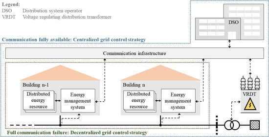
In this article, we present a multi-agent system (MAS) consisting of the BEMSs of smart buildings comprising multiple DERs, such as photovoltaics (PV)-systems, EVs, battery energy storage systems (BESSs), heat pumps (HPs), combined heat and power plants (CHPP), and intelligent appliances, a central grid controller, operated by the DSO, and the local controller of a distribution transformer. The utilized transformer can either be non-controllable or a voltage regulation distribution transformer (VRDT). The presented MAS is able to coordinate the provision of ASs for the local distribution grid in a centralized way, coordinated by the DSO, as well as in a completely decentralized way, where each building makes independent control decisions based solely on locally measurable grid status data. The MAS, as well as the different control strategies, provide the foundation for a fully adaptive grid control system, which we plan to implement and evaluate in the future, that is not only able to provide resilience against electricity outages but also against communication failures, by appropriate switching of strategies. The decentralized strategy, developed to be employed during communication failures, could also be used exclusively, for example, in regions where suitable communication infrastructure is not available in the first place. Additionally, the evaluation of the MAS can provide valuable insights into the needed communication effort to achieve the maximum possible increase in resilience against critical grid situations that smart buildings with DERs can provide. With the presented MAS, we aim to answer the following research questions, which are based on the ones we posed in [21]:

• How far can the resilience of distribution grids be increased by utilizing the energy flexibility of buildings?
• To what extent is communication needed for the exploitation of this flexibility? What are the advantages and disadvantages of the centralized and decentralized approaches for increasing the distribution grid’s resilience? How does the centralized approach perform compared to the decentralized approach?

An overview of the contributions we provide in this article is given in

Table 1. List of the contributions of this article.

Contributions
The development of a centralized (Section 2.4.2 and Section 2.4.3) as well as a decentralized (Section 2.4.4) grid control strategy to coordinate the provision of ancillary services by smart buildings, each employing cascades of measures aimed at restricting the buildings’ normal operation as little as possible.
The provision of criteria (Section 2.4.1) and development of algorithms that enable the grid-supportive adjustment of reactive (Section 2.4.5) and active (Section 2.4.6) power by buildings for both developed grid control strategies.
The development of an MAS that supports the developed grid control strategies (Section 2.1, Section 2.2 and Section 2.3) and can be extended in the future to achieve a comprehensive grid control system that adapts to communication failures by appropriately switching control strategies.
A comparative evaluation of the developed centralized and decentralized grid control strategies and corresponding control algorithms using the developed MAS (Section 3).
The interpretation of the evaluation results (Section 3) to answer the posed research questions (Section 1) concerning the potential of exploiting energy flexibility to increase grid resilience and the needed communication effort for this exploitation.

.

This paper is structured as follows. Section 1 introduces the topic and states related work on the field with a focus on microgrid management as well as AS provision by and coordination of DERs. Section 2 presents the concepts and system architecture for the centralized and decentralized control of the DERs of smart buildings aimed at increasing the resilience of low-voltage grids. The proposed concepts are evaluated and discussed in Section 3. Finally, a conclusion is given in Section 4.

2. Materials and Methods

This section introduces the BEMS used to exploit the internal energy flexibility of buildings as well as an anticipated adaptive grid control system, for which the control strategies presented and evaluated in this article form the basis. Furthermore, it provides criteria to determine the criticality of a particular grid status and details the developed centralized and decentralized grid control strategies. Additionally, it describes the use cases for as well as the implementations of reactive power control and active power targets for both of these strategies.

2.1. The Building Energy Management System Organic Smart Home

The BEMS and building simulation software framework Organic Smart Home (OSH) [22] is used as a basis for the simulation of the smart buildings considered in this research. It uses the Observer/Controller paradigm developed in the context of the research area of Organic Computing [23], which enables self-organization and reduces the complexity of the interaction between software-controlled subsystems. The building energy management provided by the OSH enables comprehensive control of the DERs in real and simulated buildings. It uses an adaptive evolutionary algorithm to schedule intelligent appliances, BESSs, EV-charging stations, HPs, and CHPPs in an optimization encompassing multiple energy carriers [24]. The latest internal version of the OSH also enables multi-building simulations combined with power-flow studies to determine the impacts of different control strategies on the local low-voltage grid [11]. An overview of the OSH’s BEMS architecture is given in Figure 1.

In this article, the OSH is extended to allow the BEMS to receive and implement commands from the DSO meant to avoid or reduce critical grid situations when undisturbed communication between a building and the DSO is possible. With regard to situations where there is no reliable communication either because such communication is not implemented at all or because it is disturbed, the BEMS should furthermore be enabled to determine appropriate grid supporting measures independently.

2.2. Adaptive Grid Control

The multi-agent-based grid control strategies presented and evaluated in this article form the basis for an adaptive grid control system for low-voltage distribution grids, which we introduced in [21] and aim to fully implement in the future. This system is designed to provide resilience with respect to electricity outages as well as communication failures. Resilience against electricity outages is achieved by utilizing the internal energy flexibility of buildings that is made exploitable by the OSH. Resilience against communication failures is accomplished by appropriately and automatically switching grid control strategies based on the current availability of communication infrastructure. For this purpose, in [21], three grid control strategies are proposed, each utilizing different communication schemes. The centralized control strategy is active as long as all communication links function reliably. Here, the DSO observes the current grid status by performing power-flow studies based on data communicated by the buildings connected to the grid. If a critical grid situation is detected, the DSO sends commands to the buildings and, if available, a VRDT aimed at reducing or resolving the criticality.

To achieve adaptivity in response to communication failures, the buildings continuously monitor locally measurable grid status data like the voltage at their grid connection and their own power consumption or feed-in. These status data are not only communicated to the DSO but also to other buildings and the transformer. This allows a building to perform regular power-flow studies (see also Section 2.3) similar to the one performed by the DSO. If the buildings detect a critical grid situation but do not receive appropriate commands from the DSO after a certain waiting period, they can assume that the communication to the DSO is currently disturbed. If a communication failure to the DSO is detected, but the VRDT and the buildings can still communicate among themselves, these agents switch to using a consensus-based control strategy. In this strategy, the buildings and the VRDT communicate relevant locally measured data among each other and collectively decide on counter measures if they detect a critical grid situation. If all communication links fail, the buildings do not receive data from other buildings or the transformer anymore. If a building does not receive any data for a certain time period, it starts to use a fully decentralized control strategy that only uses locally measurable data to detect or infer critical situations and determine appropriate counter measures. In this case, an available VRDT ceases to react to critical voltages since it has no information on the current grid status.

While the centralized and the decentralized grid control strategies are already implemented and presented as well as evaluated in the following sections, the consensus-based strategy, as well as the automated adaption of control strategies, will be implemented and evaluated in future work. A schematic of the proposed adaptive grid control system is shown in Figure 2.

2.3. Power-Flow Simulation

For this work, the power-flow study capabilities of the OSH are used in two different contexts. On the one hand, they are used to simulate the actual low-voltage grid in the considered evaluation scenario. On the other hand, they are used for the centralized grid control strategy by the (simulated) DSO. The DSO regularly performs power-flow studies based on the power data communicated by the simulated buildings and measured at the simulated transformer to gather information about the grid status, which would otherwise have to be measured by a large amount of dedicated sensors [25]. Furthermore, the DSO can use additional power-flow studies to determine which buildings are most likely to be able to prevent or improve a certain critical grid situation in grids with ring topologies. However, for the simulated grid in this article, which is shown in Figure 3, this is not relevant because its topology is exclusively radial.

All performed studies are single-phase as an even load distribution over all three phases is assumed. A detailed description of the implementation of the power-flow study capabilities of the OSH can be found in [11].

2.4. Grid Control Logic

In the following, the control strategies used by the DSO and the buildings to prevent or improve critical grid situations are introduced. There are several ways to influence the stability of the grid using different forms of energy flexibility that residential buildings can offer. Reactive power consumption or feed-in may be modified by modern PV and BESS inverters. Reactive power can be freely adjusted within the range of the currently usable fraction of an inverter’s nominal apparent power [27], which does not impact the comfort of the inhabitants of a building. Active power consumption or feed-in can be influenced by adjusting BESS and EV charging and scheduling the operation of intelligent appliances as well as HPs and CHPPs. However, the adjustment of active power is not only constrained by device characteristics, such as BESS capacity, but also by the inhabitants’ behavior and preferences, such as target temperatures [24].

2.4.1. Critical Grid Situations and Criticality Boundaries

This paper considers three types of critical situations that are relevant in low-voltage grids. Preventing or alleviating these critical situations can consequently substantially increase the resilience of a given grid [1].

The first type of critical situation considers deviations from the permitted voltage range. According to the International Electrotechnical Commission [28], voltages in low-voltage grids have to stay within a range of ±10% around the nominal voltage. To prevent voltage range deviations due to sudden spikes in power consumption or feed-in, we propose a more narrow range of −8% to +7% for the node voltages $u_{node}$ to trigger the activation of grid control measures, which corresponds to the range that triggers voltage based red grid traffic light signals in [11]. This enables timely responses to voltages running up to critical values, even if counter measures entailing significant time delays, such as optimization, are utilized. The two boundaries differ due to the different characteristics of the loads leading to increased or decreased voltages. Increased voltages are a result of power generation exceeding consumption. Power generation in German low-voltage grids mostly stems from PV systems. The generation by PV systems frequently fluctuates due to weather changes and is highly synchronous for spatially close systems often found in low-voltage grids [29]. In contrast, decreased voltages are caused by elevated power consumption, which is generally far less synchronized than elevated generation from spatially close PV systems [30]. Consequently, since larger voltage fluctuations are to be expected if voltages are above the nominal voltage, the upper criticality boundary includes a larger security margin. While the general boundaries for voltage criticality are the same for all utilized control strategies, modified voltage levels at which certain counter measures are triggered are used for different control strategies and situations. The modifications are described in detail in Section 2.4.2, Section 2.4.3, Section 2.4.4 and Section 2.4.5.

The second type of critical situation considered is the congestion of grid lines due to excessive power transmission entailing currents that exceed the respective rated current for prolonged time periods. Here, as in [11], a boundary of 90% of the rated current $I_{line}^{\mathrm{rated}}$ of a particular line is proposed to trigger the implementation of counter measures, which gives the grid control a security margin to react before a line becomes congested.

The third type of critical situation is the overheating of the transformer that supplies a particular grid. Overheating due to prolonged exceedence of a transformer’s nominal power decreases the working life of the transformer. This can entail financial losses and even power outages caused by premature equipment failure [31]. As in [11], to comply with the temperature and overloading limits given in [31] and taking into account the thermal inertia introduced by the transformer oil, a winding hot-spot temperature T of 70 °C and an overloading factor $LF=\frac{I_{trafo}}{I_{trafo}^{\mathrm{rated}}}$ of 1.3 are used as boundaries for the activation of counter measures.

All defined criticality boundaries are given in

Table 2. Criticality boundaries that trigger counter measures. Adapted from ref. [11].

Critical Situation Type	Relevant Quantities	Criticality Boundaries
Voltage range deviations	Node voltage $u_{node}$	$u_{node}<0.92\mathrm{pu}\vee u_{node}>1.07\mathrm{pu}$
Grid line congestion	Line current $I_{line}$	$I_{line}>0.9·I_{line}^{\mathrm{rated}}$
Transformer overheating	Winding hot-spot temperature T and load factor LF	$T>70 °\mathrm{C}\vee LF>1.3$

. For readability and generalizability, in this article, voltages are always given as pu, which stands for per unit and constitutes a normalization of the voltage to the nominal voltage of a given grid.

2.4.2. Centralized Control Strategy

In the centralized grid control strategy, the central controller of the DSO does not solve an optimal power flow problem for the entire grid. All optimization needed to achieve grid supportive behavior is conducted individually by the local BEMS of each building. The central controller is only responsible for observing the grid status based on data communicated by the buildings, determining which buildings should provide ancillary services in a critical situation, and the calculation of reactive power targets for each building according to the algorithm shown in Section 2.4.5. We assume that all buildings in the grid possess smart meters and smart meter gateways or similar systems, which enable them to measure and communicate the power at their own grid connection to the DSO as well as receive commands from the DSO. This assumption is supported by the Technical Guideline for the Communication Unit of Intelligent Metering Systems issued by the German Federal Office for Information Security (BSI) [32] and the German Metering Point Operation Law [33]. According to [33], in Germany, smart meters have to be deployed for all new installations and smart meter gateways for all consumers with a power consumption of more than 6000 kWh/a or with more than 7 kW_p of renewable energy feed-in. This is true for all buildings considered in this article since the combined peak feed-in from the PV system and the BESS is always higher than 7 kW_p. Several options to integrate EMSs, such as the OSH, into the German smart meter gateway infrastructure, and thereby enable secure communication between these EMSs and external entities, have been detailed by Förderer et al. [34]. Kroener et al. presented a prototype that enables the communication of demand side management measures by an external entity and their implementation by a local EMS for an EV-charging station using the German smart meter gateway infrastructure [35]. Compared to other countries, the smart meter roll out in Germany started relatively late [36] due to the high standards with respect to privacy, security, and functionality stipulated by the BSI [37]. Therefore, we assume similar infrastructure to be present in other regions as well. We furthermore assume that the metering and the communication systems can provide measurements with a one-minute resolution so that the DSO can perform power-flow studies with a one-minute resolution as well. This eliminates the need for dedicated sensors to obtain comprehensive grid status data and makes the approach scalable.

The aim of the centralized strategy is to use the full potential of the energy flexibility buildings can provide to prevent critical situations while keeping restrictions of their normal behavior, such as market interaction or energy cost minimization, to a minimum. This requires a defined cascade of measures to be taken for each type of critical grid situation. The cascades of measures for voltage as well as congestion management, which are partially adapted from [11], are detailed in Figure 4. The main differences to the proposals in [11] are in the specific execution. While [11] uses variable electricity prices for both reactive and active power to incentivize buildings to act in a grid supporting way, we propose a direct implementation of specific reactive and active power targets and differentiate between reactive power for voltage regulation and reactive power compensation to maximize the exploitation of the available flexibility, if necessary. Our description of the active power flexibility a building can provide and the mechanism of ranking the flexibilities of multiple households are inspired by the definitions and mechanisms utilized in [11] as well, but they are fundamentally adjusted to account for the target-based flexibility calls.

In the case of critical voltages, a VRDT can be used if one is available. By changing the transmission ratio of the VRDT, the voltages in the supplied grid can be adjusted in a certain range as long as all voltages in the grid stay within accepted margins [38]. If only voltages are critical and the grid is supplied by a VRDT, the latter should be used before the buildings start to intervene, as this does not affect their free market interaction.

If the provision of ASs by buildings is necessary, it should be ensured that they improve the current grid status rather than not being effective or even impairing it further. For this reason, the DSO first determines which buildings can potentially influence the critical situation in a similar way as in [11]. If a building is located within a certain distance from a node with a critical voltage, it is assumed to be able to influence the critical voltage. This distance may be varied depending on the size of the grid and the magnitude of a particular critical situation in future iterations of the centralized strategy. In [11], it was estimated that buildings within a distance from a critical node of 5% of the total number of nodes in a given grid would be able to appreciably influence this critical node’s voltage. For voltages above 1.07 pu, which we use as a criticality boundary in this article (see also Section 2.4.1), they doubled this distance. For the 62-node grid used in the evaluation, this would correspond to a distance of six nodes. For the evaluation in this article, we instead use a distance of eight nodes, since, during development, this resulted in a better ability of the centralized strategy to keep node voltages below 1.07 pu without leading to significant overreactions to critical voltages. We aim to conduct a more detailed analysis of the influence of the distance setting in future research after implementing further improvements to the centralized strategy based on the findings of this article. We assume that, at the current stage of development, a detailed parameter study would not contribute significantly to the performance of the presented strategy and that it would have to be performed again after further development. Concretely, for the grid shown in Figure 3, a distance of eight nodes means that the building connected to node three is still considered to be able to potentially influence the voltage at node eleven. For line congestions, as in [11], any building separated from the transformer by the congested line segment is expected to potentially be able to improve the situation. When it comes to critical transformer temperatures, all buildings in the grid supplied by the transformer can be able to decrease its utilization. After potential candidates are determined, depending on the type and location of the critical situation, the DSO sends them commands related to the adjustment of reactive or active power.

The adjustment of reactive power (see Section 2.4.5) should be preferred over the adjustment of active power since the provision of reactive power usually does not restrict the behavior of residential buildings with respect to active power and can be influenced more immediately and unrestrictedly [11]. For congestions, this means that the reactive power consumed or fed-in by a building is locally compensated by an inverter if available. This reduces the load on the grid, as only active power has to be transmitted between the particular building and the transformer. Reactive power compensation should not be confused with reactive power control for voltage regulation. The latter is used to lower critically high or increase critically low voltages via consumption or feed-in of inductive reactive power, respectively [27]. Since deviations from the admissible voltage range can lead to electricity outages and potential damage to devices of electricity customers [39], while congestions can be temporarily compensated by the thermal inertia of grid components [31,40], reactive power compensation has lower priority and is only used if voltages are uncritical or a VRDT can be used for voltage regulation. The implementation of reactive power control for both use cases and both presented grid control strategies are detailed in Section 2.4.5.

If the adjustment of active power is necessary because the adjustment of reactive power does not resolve a critical situation, the DSO commands all buildings b in {1;2;…;B} that can potentially influence the critical situation to determine and communicate their current active power flexibility. To calculate its flexibility, each building first schedules its device usage according to its current optimization objective, which, in this article, is the minimization of energy costs for the following 24 h, and saves the values $P_{b,t}^{\mathrm{cost}-\mathrm{opt}}$ of the resulting cost-optimized load profile. The particular temporal resolution for the optimized load profiles used for the evaluation in this article is five minutes. Higher resolutions substantially increase the computational cost and do not significantly improve the optimization [41]. After the cost-optimized load profile is determined, the building schedules its device usage again for the same schedule horizon, but this time using an active power target $P^{\mathrm{tar}}$ for the duration of all time steps t in the active power target horizon T. Note that T does not have to be equal to the scheduling horizon. We do not use an index variable indicating different time steps for $P^{\mathrm{tar}}$ because, in the context of this article, the target always has the same value. The reasons for this as well as the scheduling according to an active power target are detailed in Section 2.4.6. When the resulting values $P_{b,t}^{\mathrm{tar}-\mathrm{opt}}$ of the target-optimized load profile are determined, they are compared to the ones in the cost-optimized load profile, and the flexibility $F_b$ is calculated using Equation (1):

$$F_b=\sum _{t=1}^T\left({\left(P_{b,t}^{\mathrm{cost}-\mathrm{opt}}-P^{\mathrm{tar}}\right)}^2-{\left(P_{b,t}^{\mathrm{tar}-\mathrm{opt}}-P^{\mathrm{tar}}\right)}^2\right).$$

(1)

Both terms inside the sum are squared so that higher deviations from the active power target are weighted higher than lower deviations. This is aimed at reducing load peaks that lead to especially high equipment utilization and voltage fluctuations. An $F_b$ of zero or below means that the implementation of the target-optimized load profile would not improve the grid status and the building should continue acting as if it was uncritical. An $F_b$ below zero can occur due to the functionality of the utilized evolutionary algorithm, which is aimed at finding good solutions within a short time as opposed to finding optimal solutions. This functionality is utilized because, in real applications, building optimization algorithms often have to run on low-cost, low-energy computers and repeatedly throughout the day. Furthermore, the uncertainty associated with the optimization of the energy flows of a building diminishes the advantages of optimal over good solutions [42]. However, this can lead to certain cost-optimized load profiles being nearer to an active power target on average than certain target-optimized load profiles by accident, especially, if the current flexibility of the building is low. If this happens, the current flexibility of a building is assumed to be zero. A positive $F_b$ indicates that the building can improve the grid status and enables a comparison with the flexibility of other buildings.

When the buildings have calculated their respective flexibilities, they communicate them to the DSO, which then calls the flexibility of a group of the most flexible buildings, by commanding them to implement their respective target-optimized load profiles. For the purpose of the evaluation in this article, the group size is set to five. We plan to analyze the influence of the group size on the performance of the centralized strategy in the future. If the grid status is still critical after the buildings start to implement the active power target, the DSO calls the next group of buildings. This process repeats until the critical situation is resolved or all relevant buildings are already implementing an active power target.

Control options that enable the DSO to demand and the buildings to implement forcible load curtailment, for example, of the power generation by PV systems or the charging of EVs, if the available flexibility is not sufficient to resolve a critical situation, are planned for future research and not yet implemented.

2.4.3. Voltage Regulated Distribution Transformer

The control algorithm used for the VRDT is partially based on the control algorithm developed and implemented in [43]. The original algorithm only considers voltage range deviations above an upper criticality boundary. For this work, the algorithm is extended to also cover voltages that fall below a lower criticality boundary. Changes in the VRDT’s transmission ratio are triggered at different upper and lower voltage set points depending on the spread between the maximum and minimum node voltage in the grid. In the utilized algorithm, dead bands are used to prevent the transmission ratio from oscillating. When one or more node voltages in the grid exceed the quick dead band on top of the higher voltage set point, the transmission ratio is switched up immediately. When the voltage only exceeds the slow dead band on top of the higher voltage set point, the transmission ratio is switched up after a waiting period, during which the voltage has to continuously stay above the slow dead band. For the evaluation in this article, the same waiting period of five minutes as in [43] is used. In future research, the influence of this parameter could be analyzed in detail. If one or more node voltages in the grid reach the lower voltage set point, the process of changing the transmission ratio works analogously to the one for high voltages but in the other direction. All parameters used for the voltage regulation by the VRDT utilized in this paper are given in

Table 3. Control parameters for the VRDT. Partially adapted from ref. [43].

Condition	Parameter	Value
$u_{node}^{\max }-u_{node}^{\min }>0.1\mathrm{pu}$	Higher voltage set point	1.07 pu
	Lower voltage set point	0.925 pu
	Slow dead band	0.015 pu (300 s waiting time)
	Quick dead band	0.02 pu (immediate)
$u_{node}^{\max }-u_{node}^{\min }\le 0.1\mathrm{pu}$	Higher voltage set point	1.05 pu
	Lower voltage set point	0.945 pu
	Slow dead band	0.02 pu (300 s waiting time)
	Quick dead band	0.04 pu (immediate)

:

2.4.4. Decentralized Control Strategy

For the decentralized grid control by the buildings based on locally measured data on the low-voltage grid, the goals are the same as for the centralized control by the DSO. The buildings should try to prevent critical situations to the fullest of their abilities while only doing so when necessary to limit their own objectives as little as possible. This requires an adjusted cascade of measures for each type of critical grid situation that can be detected or at least inferred locally. The cascades of measures for voltage as well as congestion management applied by each building are shown in Figure 5.

The decentralized control strategy assumes no communication among the buildings, the transformer, and the DSO. As a consequence, an available VRDT has no info on the local voltages at the buildings’ grid connections. An adjustment of the transmission ratio based on the voltage at the busbar could lead to local deviations from the admissible voltage range. This means that voltage regulation with a VRDT is not available in this scenario.

For the same reasons as in the central control strategy, the adjustment of reactive power is preferred over the adjustment of active power.

Since a building only knows the local grid situation, namely the voltage at its grid connection and its own power generation and consumption, it has to make control decisions based on this data. Possible congestions in the grid have to be inferred from the local voltage. Congestions arise from excessive power feed-in or draw into or from a particular grid line or the entire grid [44], which generally entails at least moderately elevated [45] or lowered voltages [46]. For this reason, the building starts to implement reactive power compensation and active power targets if the local voltage is not yet critical but moderately deviates from the nominal voltage. The upper and lower voltage levels that trigger anti-congestion measures are set to 1.03 pu and 0.95 pu in the simulations performed for this article, which correspond to the values that trigger voltage-based yellow grid traffic light signals in [11]. The lower level deviates further from the nominal voltage than the upper one because low voltages are generally more short lived than high voltages. As described in Section 2.4.1, the consumption of electricity in low-voltage grids is less synchronized than the generation. This means that congestions due to excessive consumption require a high magnitude of unlikely synchronization and thus are generally less frequent, less pronounced, and less persistent. Due to the thermal inertia provided by the transformer [31] and the possibility of momentarily exceeding a grid line’s nominal currents [40], the security margin for the lower voltage boundary can be smaller.

If the local voltage becomes critical according to Table 2, the building starts to adjust its reactive power according to the control algorithm detailed in Section 2.4.5.

When a building determines that the adjustment of reactive power cannot resolve a locally observed or inferred critical situation and active power flexibility should be used, it first calculates its active power flexibility in the same way as in the centralized control strategy (Equation (1)). If the calculated flexibility F is positive, the building starts to implement an active power target as described in Section 2.4.6.

As for the centralized control strategy, additional control options enabling the curtailment of local loads for devices that allow this are planned for future research.

2.4.5. Reactive Power Control

Reactive power can be used to influence different types of critical situations. In the context of congestions, reactive power compensation can be useful. Here, an inverter’s capability to generate or consume reactive power is used to compensate for the current reactive power consumption or feed-in of a building. This decreases or eliminates the amount of reactive power that has to be transferred by adjacent grid lines and the distribution transformer. This can be especially useful in situations where the equipment utilization is already high due to high amounts of transferred active power [27]. Despite assuming that the buildings’ inverters are able to adjust their reactive power draw or output without fixed power factors, we call all reactive power settings detailed in this section targets. This is due to the maximum apparent power a particular inverter can provide. If a reactive power target is higher than the currently remaining inverter capacity, for example, because the inverter already outputs a high magnitude of active power, the reactive power target cannot be fully implemented. In this case, the maximum currently possible reactive power output or draw is used. Each building that is commanded to compensate its reactive power by the DSO in the centralized control strategy or that autonomously determines the usefulness of reactive power compensation in the decentralized strategy calculates the reactive power target $Q_t^{\mathrm{tar}}$ for time step t according to Equation (2):

$$Q_t^{\mathrm{tar}}=Q_{t-1}^{\mathrm{tar}}-Q_{t-1}.$$

(2)

Here, $Q_t^{\mathrm{tar}}$ denotes the new target to be implemented by the inverter, $Q_{t-1}^{\mathrm{tar}}$ the previous target, and $Q_{t-1}$ the previous inductive reactive power at the building’s grid connection. Positive values for the inductive reactive power Q in this context denote consumption and negative values generation or feed-in. Since the reactive power targets for the reactive power compensation are always determined autonomously by the particular building and never communicated to or by the DSO, regardless of the chosen control strategy, we do not use a running index for different buildings in this case. For the evaluation, the duration in which the reactive power compensation stays active is chosen as eight hours, which corresponds to the duration used for the active power targets (see also Section 2.4.6). The determination of an optimal value is planned for future research.

Inductive reactive power feed-in or consumption by inverters can also be leveraged to, respectively, increase or decrease voltages in an electrical grid, which makes it an effective tool for voltage maintenance [27]. If voltages are critical according to the boundaries established in Section 2.4.1, we always prefer the use of reactive power for voltage regulation over reactive power compensation since voltage range deviations generally result in damaged equipment faster [39] than congestions [31,40]. We utilize two very similar reactive power control algorithms that are designed to limit the additional load on the grid introduced by increased transmission of reactive power while maintaining a security margin for large voltage fluctuations. One is utilized by the DSO (Algorithm 1) for each building in the centralized and the other by each building in the decentralized control strategy (Algorithm 2). In the algorithm for the decentralized control strategy, a building considers only the voltage u at its own grid connection to determine if it should use a reactive power target and its appropriate value. In contrast, the algorithm utilized by the DSO in the centralized strategy not only determines reactive power targets for all buildings with a critical voltage at their own grid connection $u_b$ but also for buildings that are situated within a certain distance from a node that exhibits a critical voltage. The maximum or minimum node voltage within this distance from a building is referred to as $u_b^{\max /\min -\mathrm{dis}}$. As explained in Section 2.4.2, the distance is set to eight nodes for the evaluation in this article. The DSO only communicates changed targets to the buildings. As long as a building does not receive a new target in the centralized strategy, it uses the last target previously received. Algorithm 2 does not use an index variable for different buildings because, here, the targets are calculated autonomously by the particular building and never communicated outside. In both algorithms, the reactive power is stepped up or down with three different step sizes depending on the voltage level, the previous reactive power target, and, in the case of centralized control, the location of the largest relevant voltage deviation. Before decreasing the reactive power feed-in or consumption of the inverter again, the voltage at a building’s grid connection has to be above or below certain levels, respectively, for a certain duration or cross the nominal voltage in the opposite direction of the previously critical voltage. This is conducted to prevent a premature reduction in the reactive power adjustment in the context of highly fluctuating voltages, for example, due to rapid passing by of clouds above a PV system. For the evaluation, we chose a duration of ten minutes. As the temporal resolution utilized for the power-flow studies is one minute for the reasons stated in Section 3, ten minutes correspond to ten time steps $\tau$. The presented control algorithms have not yet been formally proven to lead to stable system behavior but show stable behavior in all previously tested scenarios, including the ones shown in Section 3. However, before deployment in a possible real-world application, we highly urge the use of appropriate safety measures and extensive testing, especially in scenarios where large voltage fluctuations can occur, which might be amplified if reactive power feed-in is not adjusted fast enough.

Algorithm 1: The determination of reactive power targets by the DSO in the centralized grid control strategy. The DSO performs this algorithm each time updated grid status data are received and for all buildings determined to be able to influence critical voltages in the grid or currently implementing a reactive power target. Positive targets denote consumption and negative targets generation of inductive reactive power.
Data:
$u_{b,t}^{\max /\min -\mathrm{dis}}$	Max./min. node voltage within certain distance from building b
$u_{b,t}$	Voltage at the grid connection of building b
$S_b^{\max }$	Max. apparent power the PV inverter of building b
$Q_{b,t-1}^{\mathrm{tar}}$	Previous reactive power target for building b
Result: $Q_{b,t}^{\mathrm{tar}}$	New reactive power target for building b

Algorithm 2: The determination of reactive power targets by a building. In the decentralized grid control strategy, eachs building performs this algorithm as soon as it obtains updated data on its local grid connection. Positive targets denote consumption and negative targets generation of inductive reactive power.
Data:
$u_t$	Voltage at the building’s grid connection
$S^{\max }$	Maximum apparent power of the PV inverter
$Q_{t-1}^{\mathrm{tar}}$	Previous reactive power target
Result: $Q_{b,t}^{\mathrm{tar}}$	New reactive power target

2.4.6. Active Power Target Implementation

The exploitation of a building’s energy flexibility to adjust its active power consumption or feed-in can be used for voltage regulation as well as reducing the utilization of grid lines and transformers [11]. This can be especially useful in situations with a high simultaneity of load, for example, arising from PV generation around noon or EV charging in the evening.

To make the flexibility of a building usable for grid stabilization purposes, its BEMS should allow for scheduling based on an active power target. In the case of the OSH, the already implemented evolutionary algorithm and device models are used in conjunction with a new objective function that was implemented in [47] and is shown in Equation (3):

$$\underset{P_t\in \mathbb{R}}{min}\frac{1}{T}\sum _{t=1}^T{\left(P_t-P^{\mathrm{tar}}\right)}^2.$$

(3)

Here, $P^{\mathrm{tar}}$ denotes the active power target and $P_t$ the expected active power at the building’s grid connection for time step $t\le T$, where T is the active power target horizon. A duration of eight hours is chosen for the active power target horizon, which corresponds to 96 time steps for the five-minute temporal resolution of the optimization, motivated in Section 2.4.2. This is aimed at preventing the premature exploitation of all available active power flexibility. Preliminary testing showed that a short time period could provide better results in the short term but often leads to significant rebound effects once the period is passed. A more detailed analysis of different target values and horizons is planned for future research. The summands in Equation (3) are squared to favor more even load profiles over ones with more load spikes. This is advantageous since new load spikes introduced by rescheduling can make a critical situation even worse, despite the new load profile being very close to a set target on average. Since an active power target may be communicated by the DSO but is always implemented autonomously by the particular building and the resulting optimized load profile is never explicitly communicated to the DSO, regardless of the currently utilized control strategy, we do not use a running index for different buildings in this case.

Preliminary testing showed that varying the magnitude of the chosen active power targets has no significant influence on the performance of the presented grid stabilization algorithms, as long as the target is sufficiently lower than the current active power consumption or feed-in of a building in a given critical situation. This is due to the limited active power flexibility [24] of a building as opposed to the high reactive power flexibility offered by inverters [27]. In a situation where grid equipment is already close to being overloaded, it is thus important to use as much active power flexibility as possible to avoid having to take more drastic measures, such as curtailing PV generation and EV charging or load shedding. Consequently, for this research, $P^{\mathrm{tar}}$ is always set to 0 W. For this reason, we do not use index variables indicating different time steps or buildings in the symbol for the active power target.

3. Results and Discussion

To evaluate and compare the methods proposed in the previous section, simulation studies are performed using the OSH’s multi-building simulation and load-flow study capabilities. To adequately measure the performance of the different grid control strategies, a scenario is needed where critical situations inevitably occur. To ensure this, a scenario with a conventionally designed grid but highly modern and generously equipped buildings in the summer, when PV generation is the highest, is chosen for the evaluation. We assume that if the proposed control strategies show a good performance in an extreme scenario such as the one chosen, they most likely perform well in less extreme scenarios as well. All simulated buildings possess intelligent appliances, a PV system, a BESS, an EV, and either an HP or a CHPP. While the building simulation runs with a temporal resolution of one second, the resolution of the power-flow studies is chosen as one minute since the most highly fluctuating simulation component is the utilized PV profile, which was measured with a one-minute resolution. As a result, the grid control algorithms work with a one-minute resolution as well. The configurations of the grid, the buildings, the evolutionary algorithm, and the temporal resolutions for the different components of the simulation are given in

Table 4. The configuration of the simulated grid and buildings, the evolutionary algorithm, and the temporal resolutions of the simulation components. The grid configuration as well as the distributions of inhabitants, PV, heating systems, and BESSs are adopted from the village grid and the the day after tomorrow scenario utilized in [11]. The average grid connection point distance is increased from 34 m to 84 m, which is a top end value for villages according to the distribution given in [48].

Parameter	Value (s)
Transformer nominal power	400 kVA
Voltage on primary side of transformer	Contains a random component as in [11]
Grid topology	Radial
Feeders	5
Distributing cabinets	5
Grid line type	NAYY 4x150 SE, buried cable
Average grid connection point distance	84 m
Grid nodes	62
Grid connection points (buildings)	55
Inhabitants per building	1–5, average: 2.927
Base load profile	H0, adjusted for weekday, Saturday, Sunday, day of the year, and number of inhabitants
Simulated appliances (additional to base load)	Dishwasher, washing machine, tumble dryer, induction hob, electric oven (probability based starting times, according to [24])
Flexible appliances	Dishwasher, washing machine, tumble dryer
PV system peak power	6–30 kWp (Inverter: 6.316 kVA–33.333 kVA)
PV system power profile	Measured at the FZI House of Living Labs in 2013, scaled to respective peak powers
BESS capacity	6–10 kWh
BESS max. active charge/discharge power	4.2–7 kW ($cos\left(\varphi \right)=1$), power exchange with grid permitted
CHPP (if no HP is used)	1 kWel ($cos\left(\varphi \right)=0.9$), 4 kWth, 5.682 kWgas
Air source HP (if no CHPP is used)	6.7 kWel ($cos\left(\varphi \right)=0.95$), coefficient of performance (COP) between 1.2 and 5.1 depending on air and hot water tank temperature
Hot water storage tank	750 L, $\theta$min/max = 60/80 °C (CHPP), 40/60 °C (HP), used for both domestic and heating hot water
EV battery capacity	85 kWh
EV max. active charge power	22 kW ($cos\left(\varphi \right)=0.99$), variable charging, no discharging, usage model developed in [49]
Evolutionary algorithm population size	100 solution candidates
Evolutionary algorithm stopping criteria	100,000 generations reached or fitness delta ≤$5\times {10}^{-5}$ for 20 generations
Random seeds (appliance and domestic hot water usage, EV driving distances, evolutionary algorithm initialization)	5 per building, different for each building
Building simulation temporal resolution	1 s
PV profile temporal resolution	1 min
Power-flow studies temporal resolution	1 min
Grid control algorithms temporal resolution	1 min
Optimization algorithm temporal resolution	5 min

.

A schematic of the simulated low-voltage grid used for the power-flow studies is given in Figure 3. The topology of this particular grid was first developed in [26] and revised in [11]. For the evaluation in this article, to ensure the occurrence of voltage range deviations, we increased the average distance between the grid connection points of the considered grid from the original value of 34 m in [11] to 84 m. While 34 m is an average value for the average distance between grid connection points in villages, 84 m represents a top end value for this average distance according to the distribution given in [48]. Additionally, we applied an MVA base value of 0.4 to the transformer impedance instead of the value 0.63, which was given in the grid specification in [11]. We assume this to be more realistic for a 400 kVA transformer since, according to [50], the permissible efficiency of a transformer, which is determined by its impedance, decreases with decreasing nominal power.

To gain a meaningful assessment of the abilities of the different grid control strategies utilized depending on the availability of communication infrastructure, we simulate the entire first week of July five times for each control strategy using five different random seeds per building and differing random seeds among the buildings. The random seeds are used for the appliance, domestic hot water, and EV usage, as well as the initialization of the evolutionary algorithm. 30 June and 8 July are simulated as well, but the results for these days are discarded. This extension of the simulated time span ensures realistic initial states of charge (SoCs) for the BESSs and EVs as well as initial temperatures for the hot water storage tanks at the beginning of the week and prevents unrealistic building behavior caused by the rolling horizon optimizations the buildings utilize at the end of the week.

The simulation studies are performed on a compute cluster. Each simulation run is performed on six Intel Xeon Gold 6230 cores with activated hyperthreading, clocked at 2.1 GHz and 12 GB of Memory. Using this hardware configuration, one simulation run takes between 6.1 and 12.5 h, depending on the considered control strategy and the randomized building behavior. The data generated by the simulations is publicly available at KITopen [51].

To visualize the effects of and the significant differences between the control strategies, the progressions of the maximum local voltage in the grid, the transformer winding hot-spot temperature, and the maximum local line current in the grid are plotted for 1 July. To make the progressions for the different control strategies comparable, the results shown in the following figures are based on the same random seed configuration for every strategy. To simplify the presentation, voltages and line currents are normalized to their respective nominal values. The respective maximum sustainable values are indicated by red dotted lines. The maximum sustained value of 120 °C for the winding hot-spot temperature of the transformer is taken from [31] and the admissible voltage range of ±10% from [28]. As a point of reference, the progressions that result from using no flexibility-based grid control strategy are plotted as well.

The progressions for the different control strategies, if only reactive power control and no active power targets are used to influence critical situations, are shown in Figure 6.

The reactive power control is able to prevent all voltage range deviations in the considered time period, regardless of whether centralized or decentralized control is utilized. Since the centralized approach also includes nodes with critical voltages within a certain distance from a building in the control algorithm, it is able to more reliably stay below the upper criticality boundary of 1.07 pu than the decentralized approach. However, at least in this case, this does not inhibit the decentralized strategy from preventing all voltage deviations from the admissible range that would otherwise occur. If a VRDT is used, all voltages stay within the admissible range as well. Here, it does not matter if the VRDT is used with or without centralized reactive power control since the cascade of measures defined in Section 2.4.2 favors VRDT usage over reactive power control. As a consequence, the corresponding voltage progressions, as well as the other progressions, are almost identical.

The transformer temperature and maximum line current progressions show that the prevention of voltage range deviations comes at a price. Both the centralized and decentralized control strategies produce significantly more frequent and pronounced congestions due to the additional transmitted reactive power. Here, the decentralized strategy is at an advantage as the buildings do not consider critical voltages in their neighborhood and thus feed-in or draw less reactive power as they would in the centralized strategy.

Changing the VRDT’s transmission ratio to enable lower voltages entails higher currents and consequent losses on its windings and all grid lines, as the same power has to be transmitted. Hence, the transformer temperature and the line current are elevated when using a VRDT as well. While the increase in line current is more moderate, the increase in transformer temperature ranges between the centralized and decentralized strategies. For the lifetime of the transformer, the decentralized reactive power control strategy might consequently be slightly advantageous compared to using a VRDT.

Figure 7 shows the progressions that result from using only active power targets and no reactive power control.

In this configuration, the centralized and the decentralized control strategies perform very similarly on this particular simulated day. However, as the aggregated results, shown later in this section, indicate, this is an exception rather than the rule. This becomes apparent when taking the average SoCs of the buildings’ BESSs into consideration. Different initial BESS SoCs at the beginning of a particular day can arise from different random seeds and utilized control strategies that influence the charging behavior in the prior days. For the progressions shown in Figure 7, the average initial SoC of the buildings’ BESSs for the decentralized strategy is 37%, while it is 29% for the centralized strategy without a VRDT and 16% if a VRDT is used. As a consequence, in this particular case, the centralized strategy has more available active power flexibility it can utilize to improve critical situations, which coincidentally approximately compensates for a different effect that, by contrast, benefits the decentralized strategy. This effect stems from the different indicators used to trigger counter measures against congestions (see Section 2.4.2 and Section 2.4.4). Since, in the decentralized strategy, a building starts to implement an active power target already at relatively low deviations from the nominal voltage, power targets are generally implemented earlier. This gives the buildings time to fully discharge already partially charged BESSs and prevents fully discharged BESSs from charging too early before the grid status becomes critical. The lower SoC can then be used to decrease the highest PV feed-in powers later in the day more substantially and for longer time periods, as the BESSs can charge with higher power and for longer durations. This indicates potential for improving the centralized strategy but also shows the viability of the decentralized strategy as well as the usefulness of the local voltage as an indicator for all considered types of critical situations. For other days and random seeds, preconditions, such as the initial SoCs, could be significantly different, which potentially enables the decentralized strategy to perform better than the centralized one. This underlines the importance of using multiple random seeds and days to comprehensively evaluate the performance of the proposed strategies.

Voltage range deviations can not be fully prevented by using only active power targets. However, they can be reduced in their average magnitude for the progressions shown and could potentially also reduce their frequency for lower overall loads. Here, the additional usage of reactive power would be helpful to prevent the remaining deviations. If the centralized strategy also includes a VRDT, all deviations are prevented.

In this configuration, the control strategies that use the buildings’ flexibility show very strong performance in reducing the transformer temperature and the maximum line current, especially compared to the scenarios where a VRDT is used for voltage regulation. The reductions are so substantial that almost all congestions are prevented. This shows the potential of exploiting the flexibility modern buildings can provide when it comes to increasing the resilience of low-voltage grids without resorting to grid expansion or forcible load curtailment.

Finally, the progressions resulting from a combination of reactive and active power adjustment are shown in Figure 8.

Here, the centralized strategy performs better when it comes to reducing voltages but not in a meaningful way since the decentralized strategy still manages to keep even the highest voltages inside the admissible range for the considered time period.

Both strategies are able to substantially reduce the transformer temperature compared to the scenarios without a control strategy that uses building flexibility, especially for the one where a VRDT is used for voltage regulation. The substantial improvement also compared to the temperature progressions for the purely reactive power-based voltage control in Figure 6 stems not only from the lower load generated by active power. It also emerges from the reduced need for utilizing reactive power resulting from the lower voltages that this smaller active load induces.

As a result of the lower amount of reactive power transmitted when using the decentralized control strategy, the decentralized strategy should technically outperform the centralized strategy when it comes to reducing the transformer temperature. This is the case in Figure 6, where only reactive power control is used. However, when both control options are used, the decentralized strategy performs worse on this particular day. The reason for this behavior is the same as for the behavior previously observed in Figure 7. In this case, the described effect is even stronger, as the average initial SoC of the buildings’ BESSs for the decentralized strategy is 36%, while it is 18% for the centralized strategy without a VRDT and 21% if a VRDT is used.

Despite the aforementioned obstacles, the decentralized approach still outperforms the centralized strategy in reducing line currents as long as no VRDT is used. However, the use of a VRDT almost eliminates the additional transmission of reactive power via grid lines and thus keeps line currents substantially lower than the decentralized strategy and the centralized strategy without a VRDT.

To give a performance overview of all tested control strategies,

Table 5. An overview of the simulation results for all grid control strategies and options. The outage time corresponds to the percentage of time when one or more grid status variables are outside of the admissible range at one or more locations in the grid.

Control Strategy	Control Options
	Reactive Power Control		Active Power Targets		Both
	Outage Time	Relative Change	Outage Time	Relative Change	Outage Time	Relative Change
	One or more node voltages outside of admissible range (+/−10%)
None	3.3093%	-	3.3093%	-	3.3093%	-
None + VRDT	0.0212%	−99.36%	0.0212%	−99.36%	0.0212%	−99.36%
Centralized	0.0032%	−99.90%	2.9302%	−11.45%	0.0034%	−99.90%
Centralized + VRDT	0.0216%	−99.35%	0.0121%	−99.63%	0.0139%	−99.58%
Decentralized	0.0049%	−99.85%	2.8370%	−14.27%	0.0029%	−99.91%
	Admissible sustained transformer temperature (120 °C) exceeded
None	7.3313%	-	7.3313%	-	7.3313%	-
None + VRDT	10.7500%	46.63%	10.7500%	46.63%	10.7500%	46.63%
Centralized	11.3512%	54.83%	3.8472%	−47.52%	8.7401%	19.22%
Centralized + VRDT	10.7321%	46.39%	8.1726%	11.47%	8.0694%	10.07%
Decentralized	10.0694%	37.35%	3.0913%	−57.83%	6.1468%	−16.16%
	Rated current of one or more lines exceeded
None	0.0366%	-	0.0366%	-	0.0366%	-
None + VRDT	0.1481%	304.33%	0.1481%	304.33%	0.1481%	304.33%
Centralized	0.7541%	1958.03%	0.0050%	−86.46%	0.7060%	1826.71%
Centralized + VRDT	0.1457%	297.56%	0.0649%	77.26%	0.0662%	80.69%
Decentralized	0.6816%	1760.20%	0.0031%	−91.52%	0.5224%	1325.81%

summarizes the deviations from all admissible grid status ranges considered in this article for the entire simulated week. The displayed values are the averages of the five different random seed configurations. The outage times, which are given in percentages, are calculated by dividing the number of all simulation time steps where a particular admissible range is violated at one or more locations in the grid by the total number of simulated time steps. The name “outage time” is chosen because all of these violations can entail electricity outages. The relative increases or reductions in outage time compared to the scenario where no grid control strategy is used are given in the relative change columns.

Table 5 shows that compromises have to be made when deciding on control options. The only option that reliably reduces all types of outage is the exclusive usage of active power targets. The (additional) usage of a VRDT or reactive power control can substantially decrease and almost eliminate voltage-based outages but also increases congestions. Hence, these voltage regulation measures should only be used in combination with active power targets, as long as transformers and grid lines are not dimensioned for significantly higher maximum load than the grid equipment in the considered simulated low-voltage grid.

A remarkable observation, already indicated in the interpretation of the previous figures, can be made when comparing the performances of the centralized and the decentralized strategy. As long as no VRDT is used, the decentralized strategy performs better or at least comparably to the centralized one, regardless of whether reactive power control, active power targets, or both are used, despite the lacking availability of comprehensive grid status data. As in Figure 6, this can partially be explained by the lower magnitudes of reactive power transferred when using the decentralized strategy due to the non-involvement of critical voltages in a building’s vicinity in its decision-making process. However, this does not explain the outperformance even when only active power targets are used. As mentioned earlier, this is an effect of the different congestion management used in the decentralized strategy, which enables preventive charging or discharging of BESSs to increase the flexibility for possible critical situations later on. This means that the performance of the centralized strategy could be improved by making it work more similarly to the decentralized one, for example, by decreasing the distance in which the voltages of neighboring nodes are included in the determination of reactive power targets. Another way could be to decrease the transformer temperature and line utilization at which counter measures are triggered even further.

In the tested scenario, the major advantage of being able to use the centralized grid control strategy is the possibility of using a VRDT, which reduces voltage range deviations almost as effectively on average as reactive power-based voltage regulation but entails substantially fewer additional grid line congestions.

4. Conclusions

In this article, we developed methods to improve the resilience of low-voltage grids by exploiting the internal energy flexibility of modern buildings with BEMSs. We presented strategies that utilize centralized as well as completely decentralized grid control in an MAS comprising the BEMSs of modern buildings, a central grid controller utilized by the DSO and the local controller of a distribution transformer, which can also be a VRDT. These strategies and the MAS form the basis for an anticipated adaptive grid control system that we plan to implement in the future. This system uses different grid control strategies depending on the availability of suitable communication infrastructure, thus providing resilience not only against electricity outages but also against communication failures. It will be able to use the centralized strategy for comprehensive observation and control by considering all relevant grid status data, as long as functioning communication infrastructure is available, as well as provide resilience against communication failures by appropriately switching to the decentralized strategy. The decentralized grid control strategy could also be used exclusively in scenarios where reliable communication infrastructure is generally unavailable.

To answer the research questions posed in Section 1, the developed strategies were evaluated in a simulated scenario designed to represent the most extreme load conditions that might occur in low-voltage grids in the future. The strategies can substantially reduce voltage range deviations, transformer temperatures, and line congestions, even during communication failures, i.e., if the decentralized strategy is used, and thereby comprehensively increase the resilience of the grid in the evaluation scenario. However, there is a trade off between the reduction of congestions and the strict adherence to the admissible voltage range. The use of reactive power or a VRDT to regulate voltages more effectively compared to utilizing only active power flexibility entails higher currents on grid lines and transformers. As a consequence, we propose using these measures only in conjunction with active power flexibility or in grids that exclusively exhibit problematic voltages.

Remarkably, the decentralized control strategy, utilized if reliable communication is unavailable, shows very competitive performance to the centralized one, even surpassing it substantially in reducing outage times triggered by congestions as long as a VRDT is not available. This can be explained by its reliance on more preemptive grid control measures. Consequently, the lower performance of the centralized strategy can potentially be improved by adjusting it to work more similarly to the decentralized one. Another advantage of the decentralized strategy is the mentioned possibility of using it exclusively to increase grid resilience even in the general absence of dedicated communication infrastructure. If used exclusively, it also provides higher degrees of privacy and autonomy for electricity customers. However, a major advantage of the centralized strategy is the possibility of using a VRDT since comprehensive grid status data is available to decide on control commands for the VRDT, which is not the case for the decentralized strategy. The usage of a VRDT can improve voltages substantially while causing fewer and less pronounced congestions than reactive power control. Consequently, the answer to the question of how much communication is needed to exploit the available flexibility depends on whether a VRDT is available or not and by how much the centralized control strategy can be improved in the future.

The observations made while evaluating the developed control strategies imply various starting points for future research. A further adjustment of the various parameters used in the strategies, especially for the centralized one, would most likely improve the performance further. In this context, it would be useful to perform parameter studies to find optimal settings. Furthermore, a consensus-based control strategy for situations where the central controller fails, but communication among buildings and the transformer is still possible, could be implemented. Here, the buildings could incorporate the data measured by other buildings and the transformer into their decision making and the local controller of a VRDT could decide on control actions based on the data communicated by the buildings. Methods that allow the buildings and the transformer to automatically detect communication failures and autonomously switch between centralized, consensus-based, and decentralized strategies have to be implemented to obtain the anticipated fully adaptive grid control system. We also plan to implement methods that allow forcible load curtailment that could be used when the exploitation of flexibility is not sufficient to resolve a critical situation. The control strategies could also be evaluated for different load scenarios, such as the winter and intermediate months or highly synchronized EV charging. In addition, it would be advantageous to quantify the amount of additional energy that can be transmitted with low-voltage grids, at least for specific scenarios, by using the flexibility of smart buildings. Such results could be useful when deciding on grid dimensioning or implementing grid extensions.

References

1. Ipakchi, A.; Albuyeh, F. Grid of the future. IEEE Power Energy Mag. 2009, 7, 52–62. [Google Scholar] [CrossRef]
2. German Federal Ministry for Economic Affairs and Energy (BMWi). Gesetz zur Digitalisierung der Energiewende. 2016. Available online: https://www.bmwi.de/Redaktion/DE/Downloads/Gesetz/gesetz-zur-digitalisierung-der-energiewende.html (accessed on 1 July 2021).
3. Callaway, D.S.; Hiskens, I.A. Achieving Controllability of Electric Loads. Proc. IEEE 2011, 99, 184–199. [Google Scholar] [CrossRef] [Green Version]
4. Lasseter, R. MicroGrids. In Proceedings of the 2002 IEEE Power Engineering Society Winter Meeting, New York, NY, USA, 27–31 January 2002; Volume 1, pp. 305–308. [Google Scholar] [CrossRef]
5. Katiraei, F.; Iravani, R.; Hatziargyriou, N.; Dimeas, A. Microgrids Management. Power Energy Mag. IEEE 2008, 6, 54–65. [Google Scholar] [CrossRef]
6. Basu, A.K.; Chowdhury, S.; Chowdhury, S.; Paul, S. Microgrids: Energy management by strategic deployment of DERs—A comprehensive survey. Renew. Sustain. Energy Rev. 2011, 15, 4348–4356. [Google Scholar] [CrossRef]
7. Meng, L.; Sanseverino, E.R.; Luna, A.; Dragicevic, T.; Vasquez, J.C.; Guerrero, J.M. Microgrid supervisory controllers and energy management systems: A literature review. Renew. Sustain. Energy Rev. 2016, 60, 1263–1273. [Google Scholar] [CrossRef]
8. Mahmoud, M.S.; Alyazidi, N.M.; Abouheaf, M.I. Adaptive intelligent techniques for microgrid control systems: A survey. Int. J. Electr. Power Energy Syst. 2017, 90, 292–305. [Google Scholar] [CrossRef]
9. Zia, M.F.; Elbouchikhi, E.; Benbouzid, M. Microgrids energy management systems: A critical review on methods, solutions, and prospects. Appl. Energy 2018, 222, 1033–1055. [Google Scholar] [CrossRef]
10. Shi, W.; Li, N.; Chu, C.; Gadh, R. Real-Time Energy Management in Microgrids. IEEE Trans. Smart Grid 2017, 8, 228–238. [Google Scholar] [CrossRef]
11. Kochanneck, S. Systemdienstleistungserbringung durch Intelligente Gebäude. 37.06.01; LK 01. Ph.D. Thesis, Karlsruhe Institute of Technology (KIT), Karlsruhe, Germany, 2019. [Google Scholar] [CrossRef]
12. Feng, C.; Wen, F.; Zhang, L.; Xu, C.; Salam, M.A.; You, S. Decentralized Energy Management of Networked Microgrid Based on Alternating-Direction Multiplier Method. Energies 2018, 11, 2555. [Google Scholar] [CrossRef] [Green Version]
13. Silani, A.; Yazdanpanah, M.J. Distributed Optimal Microgrid Energy Management with Considering Stochastic Load. IEEE Trans. Sustain. Energy 2019, 10, 729–737. [Google Scholar] [CrossRef]
14. Hosseinzadeh, M.; Schenato, L.; Garone, E. A distributed optimal power management system for microgrids with plug&play capabilities. Adv. Control Appl. 2021, 3, e65. [Google Scholar] [CrossRef]
15. Zhang, K.; Troitzsch, S.; Hanif, S.; Hamacher, T. Coordinated Market Design for Peer-to-Peer Energy Trade and Ancillary Services in Distribution Grids. IEEE Trans. Smart Grid 2020, 11, 2929–2941. [Google Scholar] [CrossRef]
16. Gottwalt, S. Managing Flexible Loads in Residential Areas. Ph.D. Thesis, Karlsruhe Institute of Technology (KIT), Karlsruhe, Germany, 2015. [Google Scholar] [CrossRef]
17. Celik, B.; Roche, R.; Suryanarayanan, S.; Bouquain, D.; Miraoui, A. Electric energy management in residential areas through coordination of multiple smart homes. Renew. Sustain. Energy Rev. 2017, 80, 260–275. [Google Scholar] [CrossRef] [Green Version]
18. Celik, B.; Roche, R.; Bouquain, D.; Miraoui, A. Decentralized neighborhood energy management with coordinated smart home energy sharing. IEEE Trans. Smart Grid 2018, 9, 6387–6397. [Google Scholar] [CrossRef] [Green Version]
19. Peng, Z.; Hao, L. Decentralized Coordination of Electric Vehicle Charging Stations for Active Power Compensation. In Proceedings of the 2017 IEEE 86th Vehicular Technology Conference (VTC-Fall), Toronto, ON, Canada, 24–27 September 2017; pp. 1–5. [Google Scholar] [CrossRef]
20. Saldaña, G.; San Martin, J.I.; Zamora, I.; Asensio, F.J.; Oñederra, O. Electric Vehicle into the Grid: Charging Methodologies Aimed at Providing Ancillary Services Considering Battery Degradation. Energies 2019, 12, 2443. [Google Scholar] [CrossRef] [Green Version]
21. Ahrens, M. Increasing Power Grid Resilience With a Multi-Agent System of Smart Buildings. Extended Abstract Submitted, Full Manuscript in Preparation.
22. Organic Smart Home Website. FZI Research Center for Information Technology. Available online: https://organicsmarthome.fzi.de/ (accessed on 29 May 2021).
23. Tomforde, S.; Prothmann, H.; Branke, J.; Hähner, J.; Mnif, M.; Müller-Schloer, C.; Richter, U.; Schmeck, H. Observation and Control of Organic Systems. In Organic Computing—A Paradigm Shift for Complex Systems; Müller-Schloer, C., Schmeck, H., Ungerer, T., Eds.; Springer: Basel, Switzerland, 2011; pp. 325–338. [Google Scholar] [CrossRef]
24. Mauser, I. Multi-Modal Building Energy Management. 37.06.01; LK 01. Ph.D. Thesis, Karlsruhe Institute of Technology (KIT), Karlsruhe, Germany, 2017. [Google Scholar] [CrossRef]
25. Phadke, A.G.; Thorp, J.S.; Adamiak, M.G. A New Measurement Technique for Tracking Voltage Phasors, Local System Frequency, and Rate of Change of Frequency. IEEE Trans. Power Appar. Syst. 1983, PAS-102, 1025–1038. [Google Scholar] [CrossRef]
26. Kochanneck, S.; Geis-Schroer, J.; Mauser, I.; Schmeck, H. Reference Scenarios for the Evaluation of the Traffic Light Concept in Low-voltage Power Systems. In Proceedings of the ETG Congress 2017, Bonn, Germany, 28–29 November 2017; VDE: Berlin, Germany, 2017; pp. 330–335. [Google Scholar]
27. SMA Website. SMA Solar Technology AG. Available online: https://www.sma.de/en/partners/knowledgebase/sma-shifts-the-phase.html (accessed on 1 July 2021).
28. IEC 60038:2009, IEC Standard Voltages; International Standard; International Electrotechnical Commission: Geneva, Switzerland, 2009.
29. Fraunhofer ISE. Recent Facts about Photovoltaics in Germany. 2021. Available online: https://www.ise.fraunhofer.de/content/dam/ise/en/documents/publications/studies/recent-facts-about-photovoltaics-in-germany.pdf (accessed on 1 July 2021).
30. Hammerschmidt, T.; Gaul, A.; Christ, T.; Rehtanz, C. Simultaneity of PV- and wind power-generation from distribution grid perspective. In Proceedings of the CIRED 2012 Workshop: Integration of Renewables into the Distribution Grid, Lisbon, Portugal, 29–30 May 2012; pp. 1–4. [Google Scholar] [CrossRef] [Green Version]
31. DIN Deutsches Institut für Normung e.V.; International Electrotechnical Commission (IEC). DIN IEC 60076-7 (VDE 0532-76-7): 2008-02, Power Transformers–Part 7: Loading Guide for Oil-Immersed Power Transformers (DIN IEC 60076-7:2005); Standard; Beuth-Verlag: Berlin, Germany, 2008. [Google Scholar]
32. German Federal Office for Information Security (BSI). Technische Richtlinie BSI TR TR-0310903109-1 Anforderungen an die Interoperabilität der Kommunikationseinheit eines Intelligenten Messsystems; Technical Guideline; German Federal Office for Information Security (BSI): Bonn, Germany, 2019. [Google Scholar]
33. Gesetz über den Messstellenbetrieb und die Datenkommunikation in Intelligenten Energienetzen; Messstellenbetriebsgesetz; MsbG. 2016. Available online: https://www.gesetze-im-internet.de/messbg/MsbG.pdf (accessed on 11 June 2021).
34. Förderer, K.; Lösch, M.; Növer, R.; Ronczka, M.; Schmeck, H. Smart Meter Gateways: Options for a BSI-Compliant Integration of Energy Management Systems. Appl. Sci. 2019, 9, 1634. [Google Scholar] [CrossRef] [Green Version]
35. Kroener, N.; Förderer, K.; Lösch, M.; Schmeck, H. State-of-the-Art Integration of Decentralized Energy Management Systems into the German Smart Meter Gateway Infrastructure. Appl. Sci. 2020, 10, 3665. [Google Scholar] [CrossRef]
36. Estermann, T.; Köppl, S.; Springmann, E. Smart Metering in Europa—Was Machen Unsere Nachbarn? FfE Forschungsstelle für Energiewirtschaft e.V.. Available online: https://www.ffe.de/themen-und-methoden/digitalisierung/914-smart-metering-in-europa-was-machen-unsere-nachbarn (accessed on 5 July 2021).
37. Bundesverband Neue Energiewirtschaft e.V. (BNE); Association of Energy Market Innovators. Smart Meter Roll-Out: The German Case. 2020. Available online: https://www.bne-online.de/en/news/article/smart-meter-roll-out-the-german-case/ (accessed on 5 July 2021).
38. Forum Netztechnik; Netzbetrieb im VDE (FNN). Voltage Regulating Distribution Transformer (VRDT)—Use in Grid Planning and Operation. 2016. Available online: https://www.vde.com/resource/blob/1570326/c4c73c2670f47f82071b81eab368b85e/hinweis–ront–download-englisch-data.pdf (accessed on 5 July 2021).
39. Seljeseth, H.; Rump, T.; Haugen, K. Overvoltage Immunity of Electrical Appliances Laboratory Test Results from 60 Appliances. In Proceedings of the 21st International Conference on Electricity Distribution, Frankfurt, Germany, 6–9 June 2011. [Google Scholar]
40. Yang, Y.; Harley, R.G.; Divan, D.; Habetler, T.G. Thermal modeling and real time overload capacity prediction of overhead power lines. In Proceedings of the 2009 IEEE International Symposium on Diagnostics for Electric Machines, Power Electronics and Drives, Cargese, France, 31 August–3 September 2009; pp. 1–7. [Google Scholar] [CrossRef]
41. Müller, J. Optimization Under Uncertainty in Building Energy Management. 37.06.01; LK 01. Ph.D. Thesis, Karlsruher Institut für Technologie (KIT), Karlsruhe, Germany, 2019. [Google Scholar] [CrossRef]
42. Mauser, I.; Müller, J.; Allerding, F.; Schmeck, H. Adaptive building energy management with multiple commodities and flexible evolutionary optimization. Renew. Energy 2016, 87, 911–921. [Google Scholar] [CrossRef]
43. Geis-Schroer, J. Integration Eines Regelbaren Ortsnetztransformators in Multi-Haushalt-Simulationen Mit Dem Organic Smart Home. Bachelor’s Thesis, Karlsruhe Institute of Technology (KIT), Karlsruhe, Germany, 2017. [Google Scholar]
44. German Federal Ministry for Economic Affairs and Energy (BMWi). What Exactly Is “Grid Congestion”? 2018. Available online: https://www.bmwi-energiewende.de/EWD/Redaktion/EN/Newsletter/2018/03/Meldung/direkt-account.html (accessed on 5 July 2021).
45. Cappelle, J.; Van Maerhem, T.; Vispoel, S.; Vanalme, J.; Verhelst, B.; Debruyne, C.; Desmet, J. Introducing small storage capacity at residential PV installations to prevent overvoltages. In Proceedings of the 2011 IEEE International Conference on Smart Grid Communications (SmartGridComm), Brussels, Belgium, 17–20 October 2011. [Google Scholar]
46. Held, L.; Uhrig, M.; Suriyah, M.R.; Leibfried, T.; Junge, E.; Lossau, S.; Konermann, M. Impact of Electric Vehicle Charging on Low-Voltage Grids and the Potential of Battery Storage as Temporary Equipment during Grid Reinforcement. In Proceedings of the 1st E-Mobility Power System Integration Symposium, Berlin, Germany, 23 October 2017. [Google Scholar]
47. Ochs, P. Dezentrale Spannungshaltung in Stromverteilnetzen durch Intelligente Gebäude. Bachelor’s Thesis, Karlsruhe Institute of Technology (KIT), Karlsruhe, Germany, 2020. [Google Scholar]
48. Kerber, G.; Witzmann, R. Statistical Distribution Grid Analysis and Reference Network Generation. EW-Mag. Für Die Energiewirtschaft 2008, 107, 22–26. [Google Scholar]
49. Hummel, G. Integration von Elektrofahrzeugen in ein Gebäudeenergiemanagementsystem. Bachelor’s Thesis, Karlsruhe Institute of Technology (KIT), Karlsruhe, Germany, 2016. [Google Scholar]
50. Siemens AG Energy Management Division. New EU Requirements for Transformers. 2015. Available online: https://assets.new.siemens.com/siemens/assets/api/uuid:0f8286f00739ec6fb1e80e51a3d0711745fcd190/new-eu-requirements-for-transformers-ecodesign-directive-en.pdf (accessed on 5 July 2021).
51. Ahrens, M. Simulation Results for the Evaluation of Strategies for an Adaptive Grid Control System Using Smart Buildings (Updated). Simul. Data 2021. [Google Scholar] [CrossRef]
Figure 1. Layered Observer/Controller-based architecture of the Organic Smart Home. Reproduced from ref. [24]. OX and CX are abbreviations for observer and controller exchange communication objects.
Energies 14 04472 g001
Figure 2. Adaptation of grid control strategies to provide resilience against communication failures. The thick lines indicate electrical connections. The thin arrows indicate communication. O stands for observer and C for controller. Adapted from ref. [21].
Energies 14 04472 g002
Figure 3. A schematic of the low-voltage grid used for the evaluation, first developed in [26]. Reproduced from ref. [11].
Energies 14 04472 g003
Figure 4. Cascades of measures against critical grid situations employed by the DSO for the controlled low-voltage grid in the centralized grid control strategy. While the general cascades of measures are partially adapted from ref. [11], this schematic is new and reflects our specific implementation.
Energies 14 04472 g004
Figure 5. Cascades of measures against critical grid situations employed by each building in the decentralized grid control strategy. While the general cascades of measures are partially adapted from ref. [11], this schematic is new and reflects our specific implementation.
Energies 14 04472 g005
Figure 6. Performance comparison of the centralized and decentralized grid control strategies. Here, only reactive power control is used. Grid status progressions without flexibility-based grid control are given as a reference. The simulated day is 1 July. For comparability, all displayed progressions are based on the same random seeds. Maximum admissible values are indicated by red, dotted lines. (a) shows the progressions of the maximum node voltage in the grid. (b) shows the progressions of the transformer temperature. (c) shows the progressions of the maximum line current in the grid.
Energies 14 04472 g006
Figure 7. Performance comparison of the centralized and decentralized grid control strategies. Here, only active power targets are used. Grid status progressions without flexibility-based grid control are given as a reference. The simulated day is 1 July. For comparability, all displayed progressions are based on the same random seeds. Maximum admissible values are indicated by red, dotted lines. (a) shows the progressions of the maximum node voltage in the grid. (b) shows the progressions of the transformer temperature. (c) shows the progressions of the maximum line current in the grid.
Energies 14 04472 g007
Figure 8. Performance comparison of the centralized and decentralized grid control strategies. Here, both reactive and active power flexibility are used. Grid status progressions without flexibility-based grid control are given as a reference. The simulated day is 1 July. For comparability, all progressions are based on the same random seeds. Maximum admissible values are indicated by red, dotted lines. (a) shows the progressions of the maximum node voltage in the grid. (b) shows the progressions of the transformer temperature. (c) shows the progressions of the maximum line current in the grid.
Energies 14 04472 g008