
A New Strategy for Improving the Accuracy of Aircraft Positioning Using DGPS Technique in Aerial Navigation


Abstract
:1. Introduction
2. Related Papers
- -
- -
- -
- -
- -
- the application of the DGPS method in monitoring the ionosphere [29],
- -
- -
- -
- -
- -
- development of weighted average model algorithms to improve the accuracy of DGPS positioning using several GNSS reference stations,
- -
- implementation of a weighting model for the following three criteria: weighting as a function of baseline (vector) length, weighting as a function of vector length error, weighting as a function of the number of tracked GPS satellites,
- -
- definition of algorithms to calculate the resultant position errors,
- -
- conducting a formal evaluation of the research results obtained in percentage terms.
3. Research Method
3.1. Basic DGPS Solution for a Single Baseline
- (a)
- process of “prediction”:where
- —the matrix of coefficients,
- —the estimated values of the designated parameters a priori from the previous step,
- —the estimated values of covariance a priori from the previous step,
- —a prediction of state value,
- —the predicted covariance values,
- —the variance matrix of the noise of the measurement process.
- (b)
- process of “correction”:where
- —the Kalman gain matrix,
- —the covariance matrix of parameters determined a posteriori,
- —the matrix of partial derivatives,
- —the covariance matrix of measurements,
- —the vector of measured values,
- —the unit matrix,
- —the parameters determined a posteriori.
- —the variance–covariance matrix of parameters in the BLh ellipsoidal frame,
- ,
- —the conversion matrix from the XYZ geocentric frame to the BLh geodetic frame,
- —the mean error for geodetic latitude B,
- —the mean error for geodetic longitude L,
- —the mean error for ellipsoidal height h.
3.2. New Solution to Improve Positioning Accuracy of DGPS Technique for Multiple Baselines
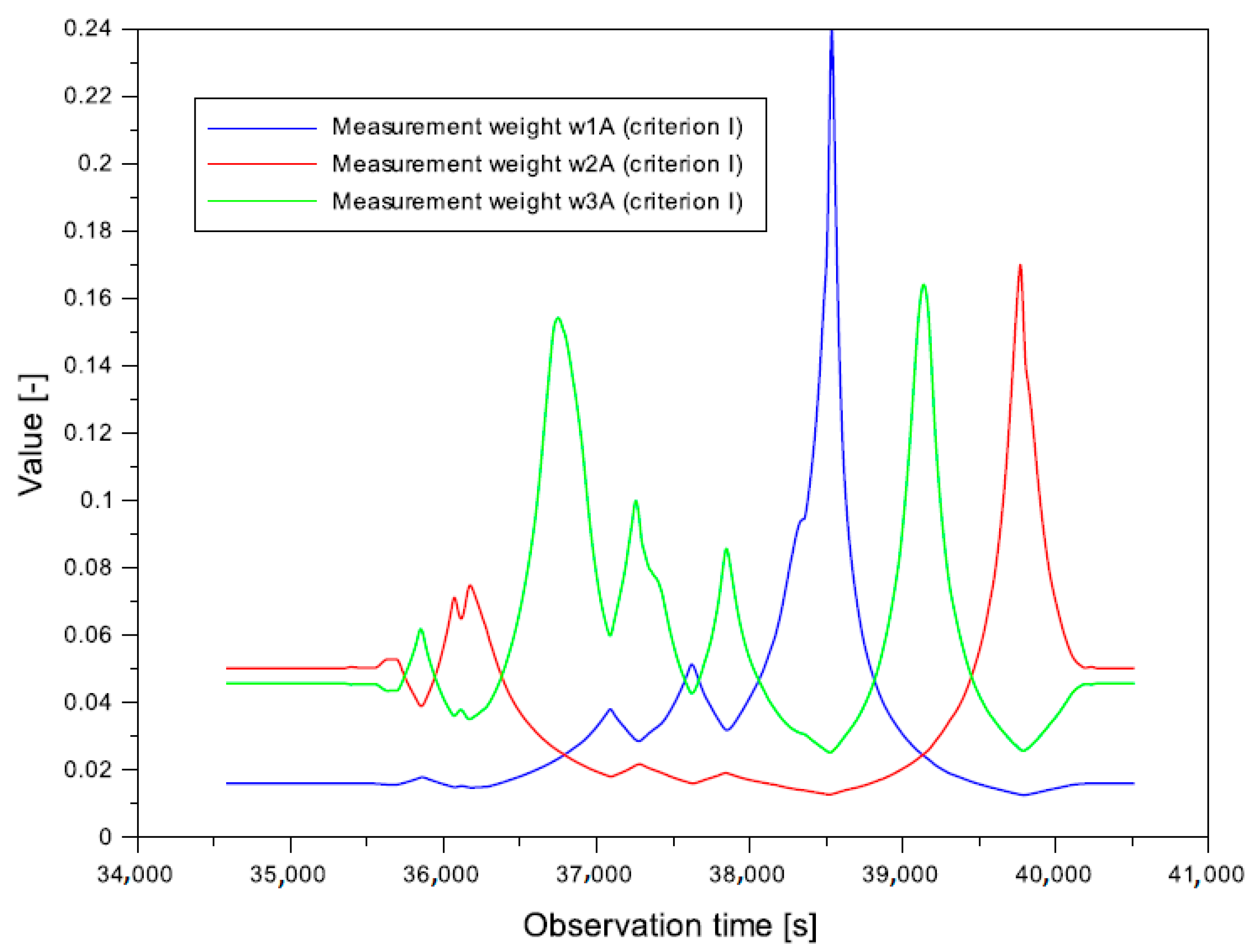
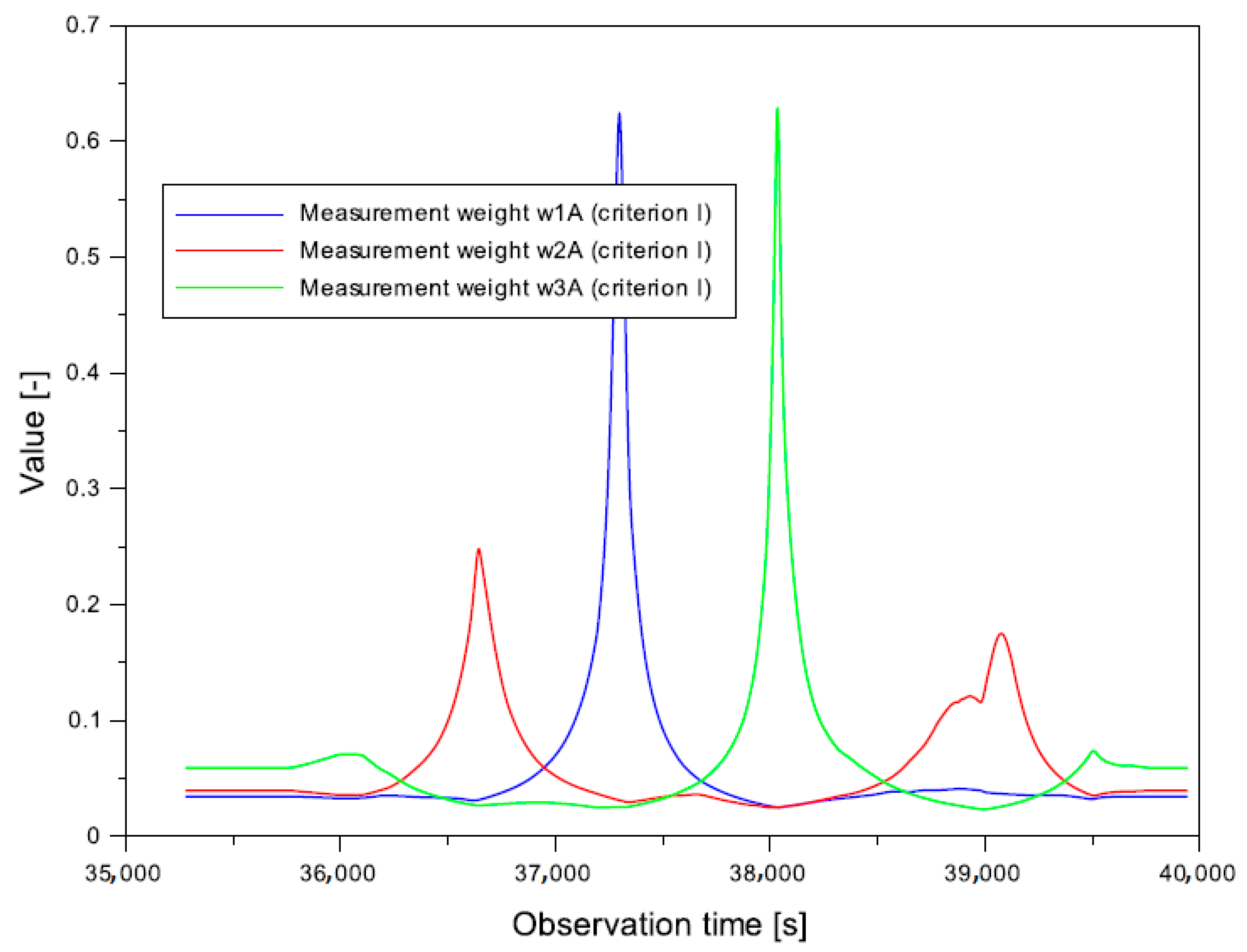
- (a)
- criterion I—weighting as a function of baseline (vector) length:where —the resultant position accuracy of the aircraft in ellipsoidal BLh coordinates; —the errors of the aircraft DGPS position in ellipsoidal BLh coordinates determined for the baseline , relative to the RTK–OTF (Real Time Kinematic–On The Fly) solution [4,43]; ; ; ; —the position of the aircraft in ellipsoidal BLh coordinates determined from the DGPS solution for the baseline (see Equation (4)); —the reference position of the aircraft in ellipsoidal BLh coordinates derived from the RTK–OTF differential technique for the baseline ; —the errors of the aircraft DGPS position in ellipsoidal BLh coordinates determined for the baseline , relative to the RTK–OTF solution; ; ; ; —the position of the aircraft in ellipsoidal BLh coordinates determined from the DGPS solution for the baseline (see Equation (4)); —the reference position of the aircraft in ellipsoidal BLh coordinates derived from the RTK–OTF differential technique for the baseline ; —the errors of the aircraft DGPS position in ellipsoidal BLh coordinates determined for the baseline , relative to the RTK–OTF solution; ; ; ; —the position of the aircraft in ellipsoidal BLh coordinates determined from the DGPS baseline solution for the baseline (see Equation (4)); —the reference position of the aircraft in ellipsoidal BLh coordinates derived from the RTK-OTF differential technique for the baseline ; —the weighting functions for individual baselines; —the baseline between the GNSS reference station () and the on-board GPS receiver (); —the baseline between the GNSS reference station () and the on-board GPS receiver (); —the baseline between the GNSS reference station () and the on-board GPS receiver (); —the distance between the GNSS reference station () and the on-board GPS receiver () expressed in geocentric cartesian coordinates XYZ; ; —the distance between the GNSS reference station () and the on-board GPS receiver () expressed in geocentric cartesian coordinates XYZ; ; —the distance between the GNSS reference station () and the on-board GPS receiver () expressed in geocentric cartesian coordinates XYZ; .
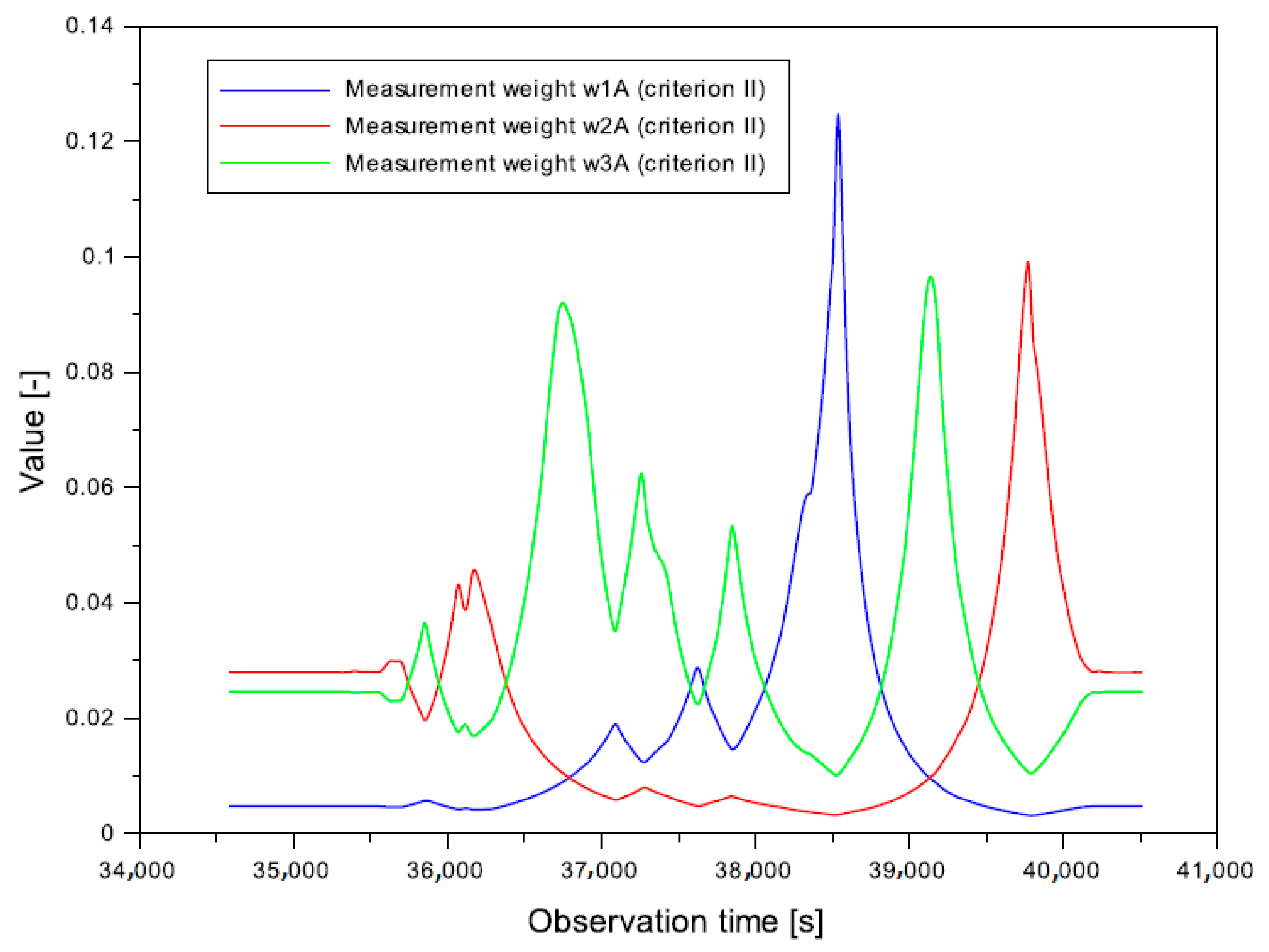
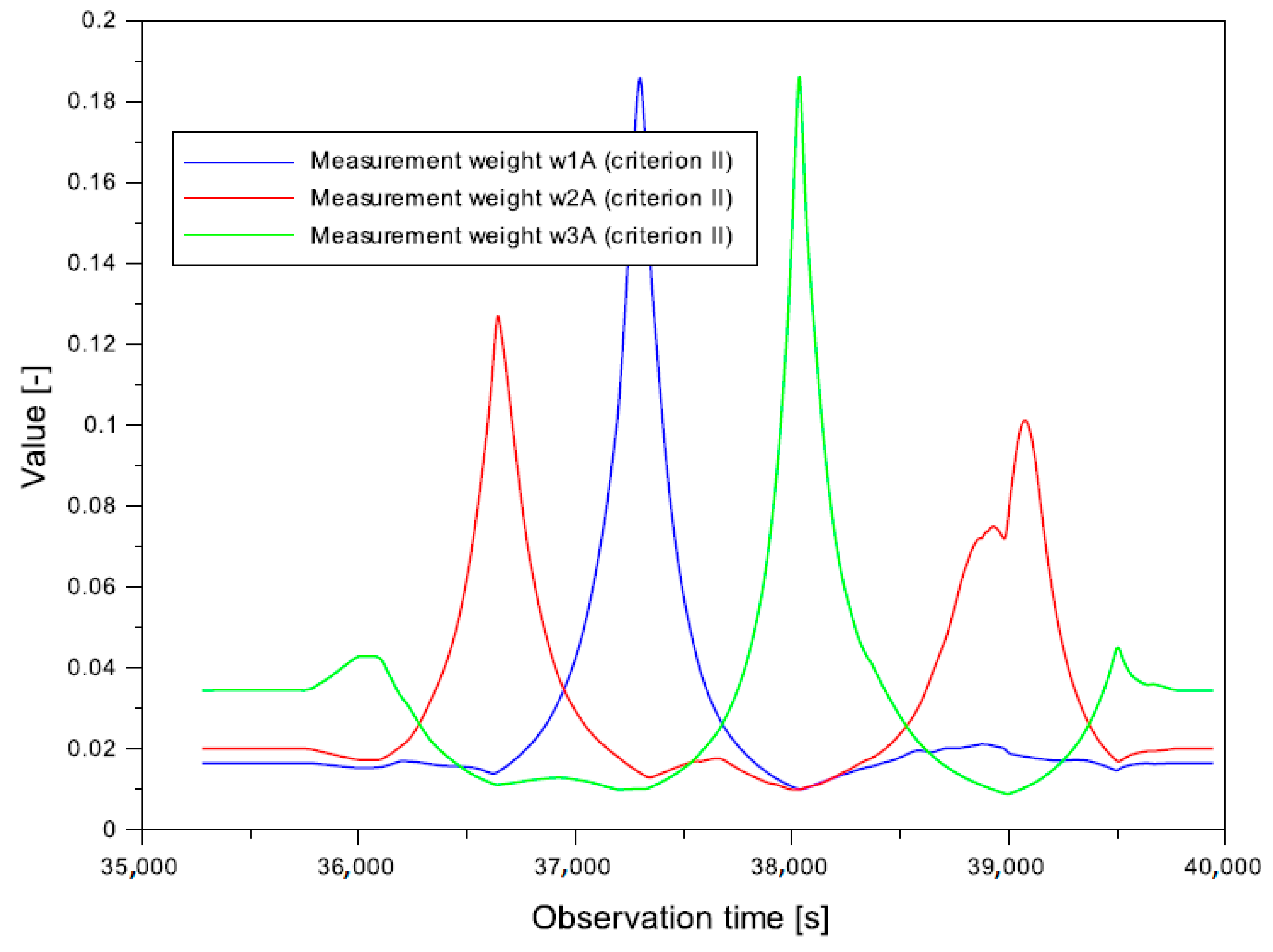
- (b)
- criterion II—weighting as a function of the error ellipse of the point position:where —the vector length error for baseline , , —the mean errors of the GNSS reference station coordinates (), —the DGPS technique assumes error-free coordinates of the GNSS reference station (), —the mean errors of the determined aircraft coordinates (), (see Equation (5)), —the vector length error for baseline , , —the mean errors of the GNSS reference station coordinates (), —the DGPS technique assumes error-free coordinates of the GNSS reference station (), —the vector length error for baseline , , —the mean errors of the GNSS reference station coordinates (), —the DGPS technique assumes error-free coordinates of the GNSS reference station ().
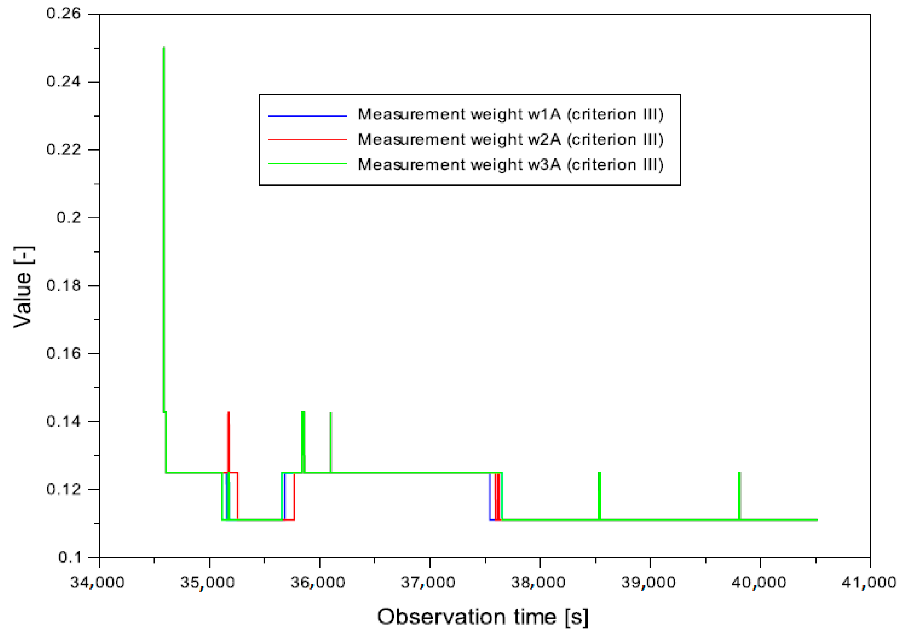
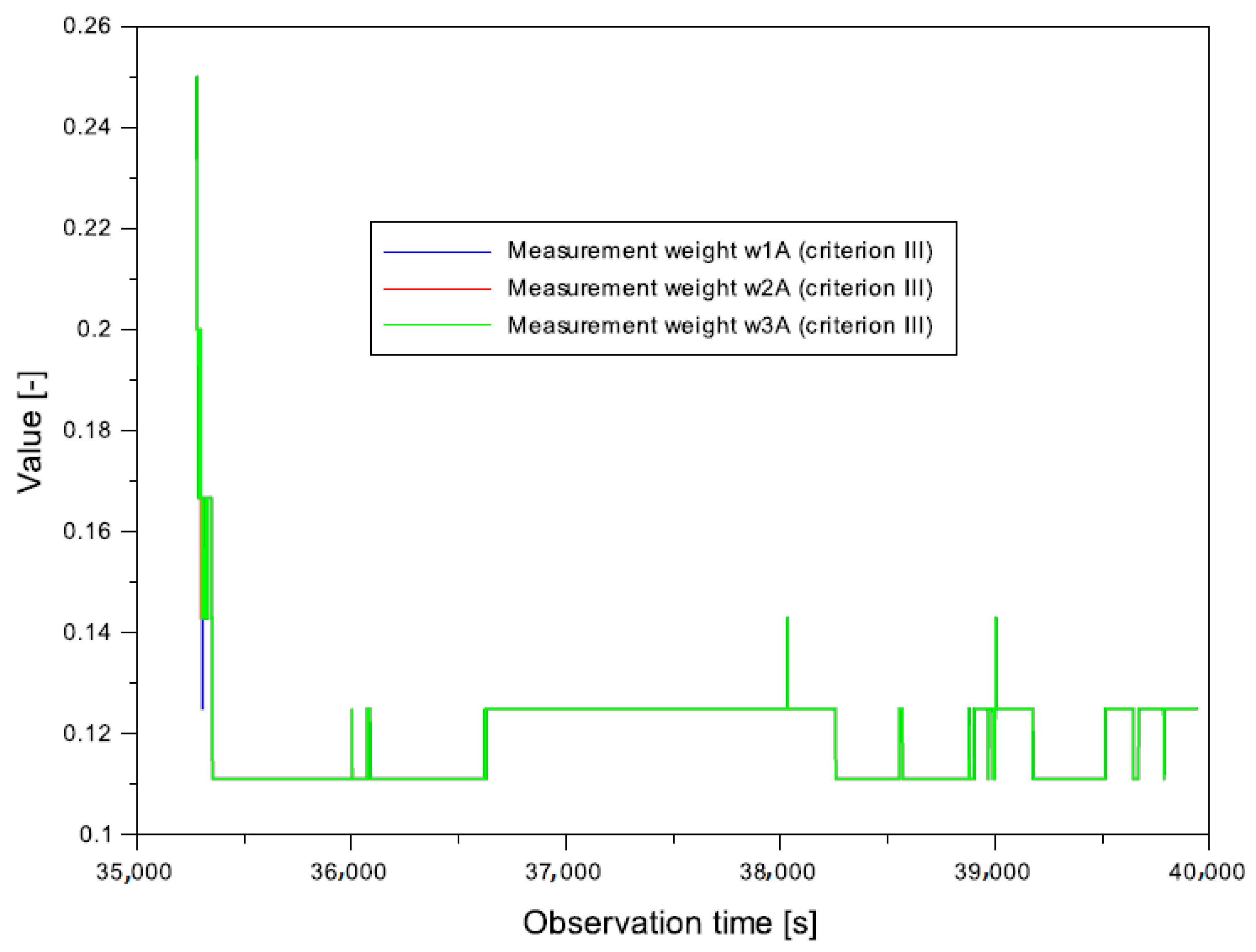
- (c)
- Criterion III—weighting as a function of the number of GPS satellites tracked:where
- —the number of tracked GPS satellites for the baseline ,
- —the number of tracked GPS satellites for the baseline ,
- —the number of tracked GPS satellites for the baseline .
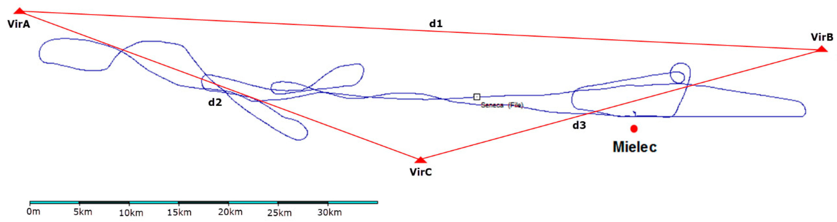
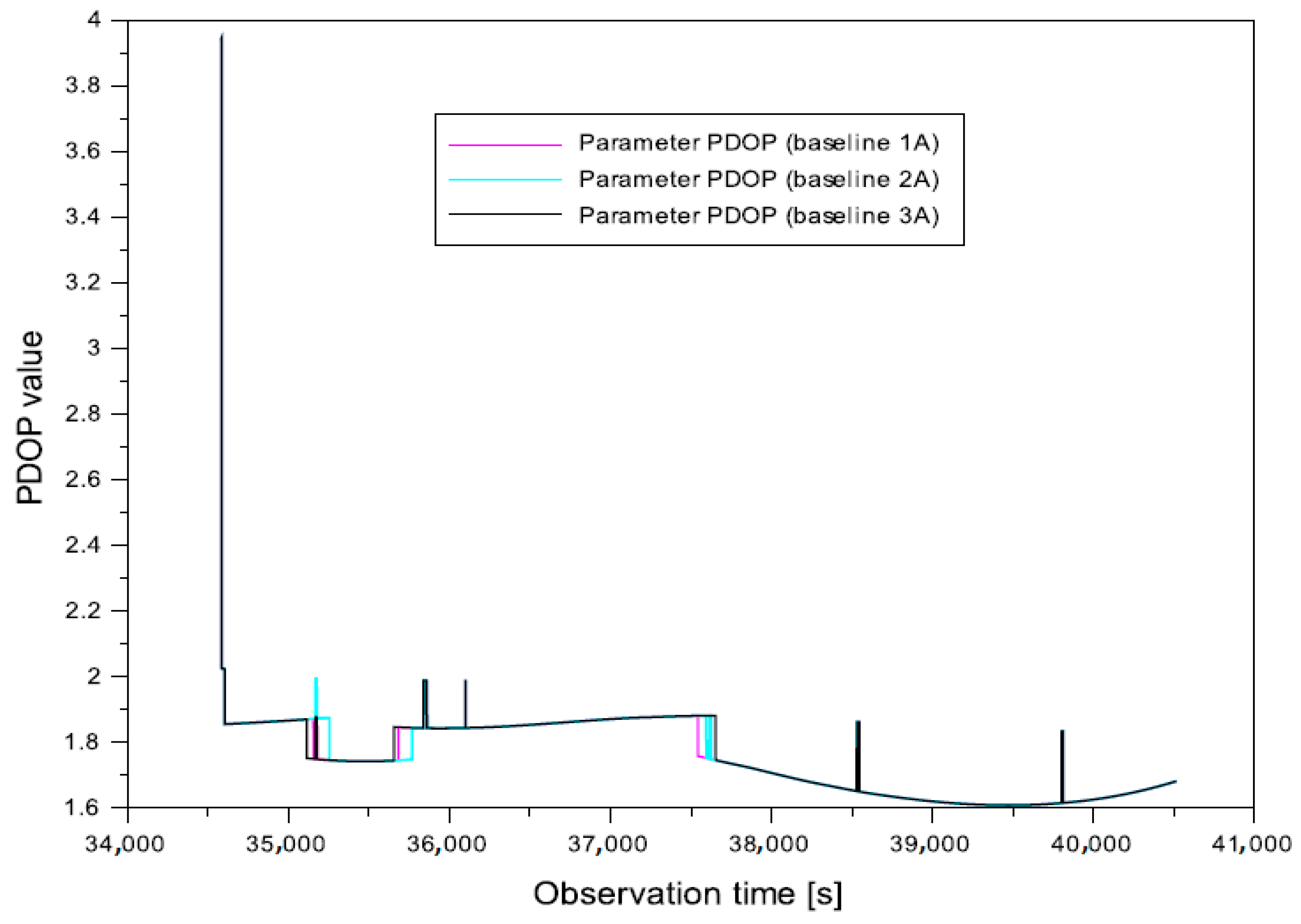
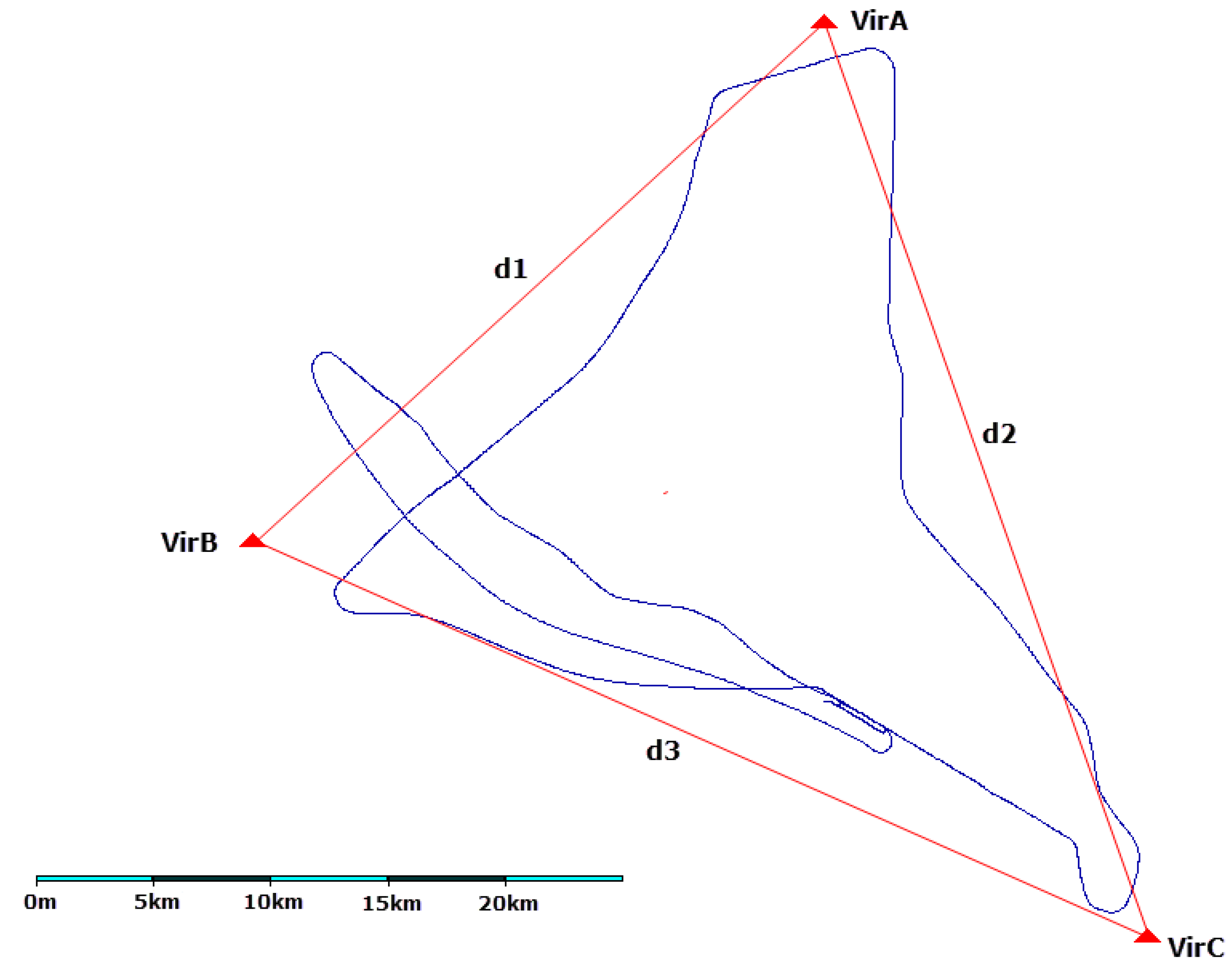
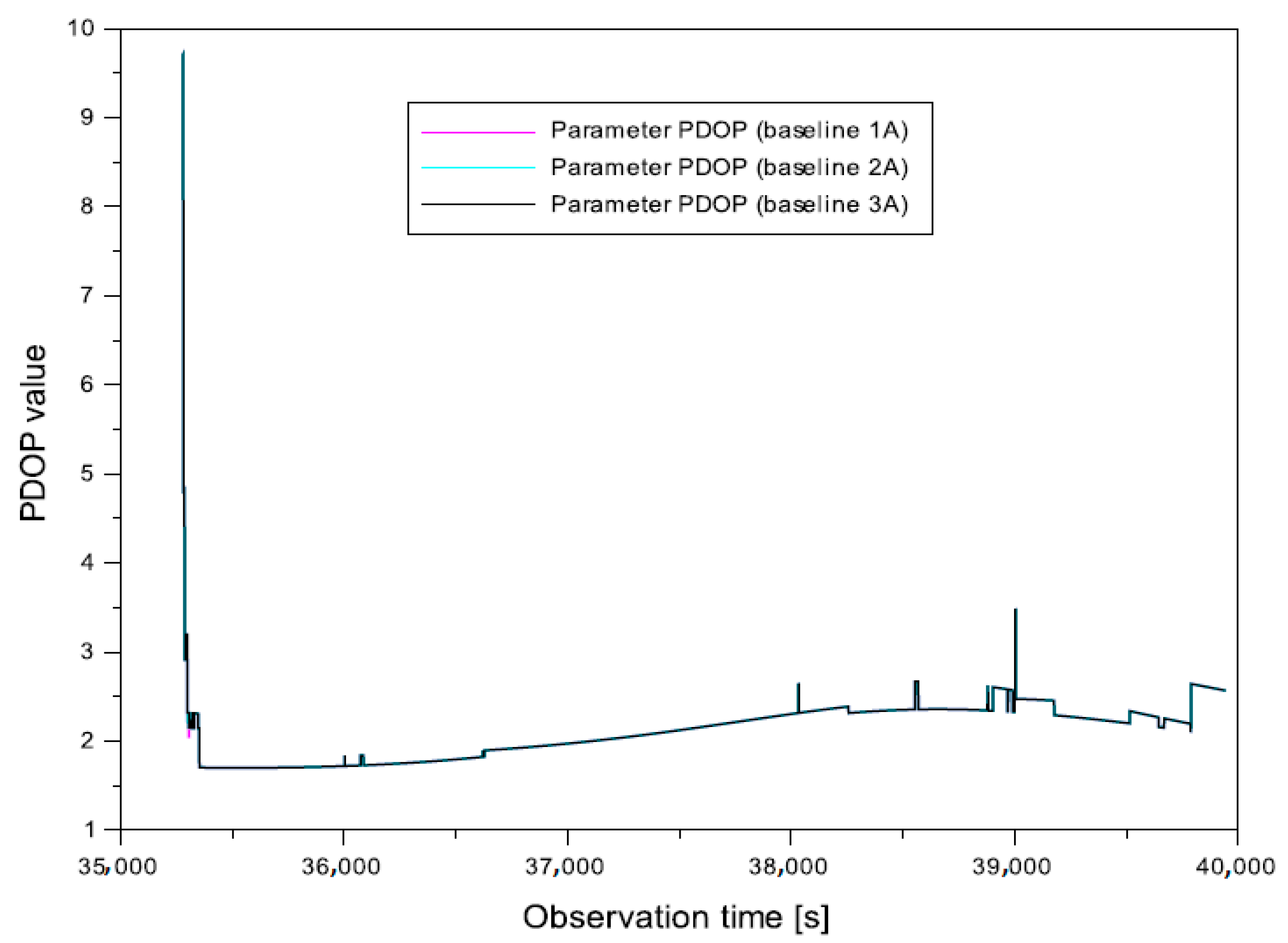
4. Research Test
- -
- 80.603 km between VirA and VirB (designation d1),
- -
- 41.918 km between stations VirA and VirC (designation d2),
- -
- 41.246 km between VirB and VirC (designation d3).
- -
- positioning mode: DGPS/DGNSS,
- -
- elevation mask: 5°,
- -
- type of filtration: forward Kalman filtration,
- -
- source of ionospheric correction: Klobuchar model,
- -
- source of tropospheric correction: Saastamoinen model,
- -
- ephemeris data source: GPS navigation message,
- -
- GNSS system: GPS system,
- -
- GPS observation type: C/A code on L1 frequency,
- -
- resulting coordinates of the aircraft position: ellipsoidal BLh coordinates,
- -
- base coordinates of the reference stations: catalogue coordinates of VirA, VirB and VirC reference stations according to Table 1,
- -
- calculation interval: 1 s.
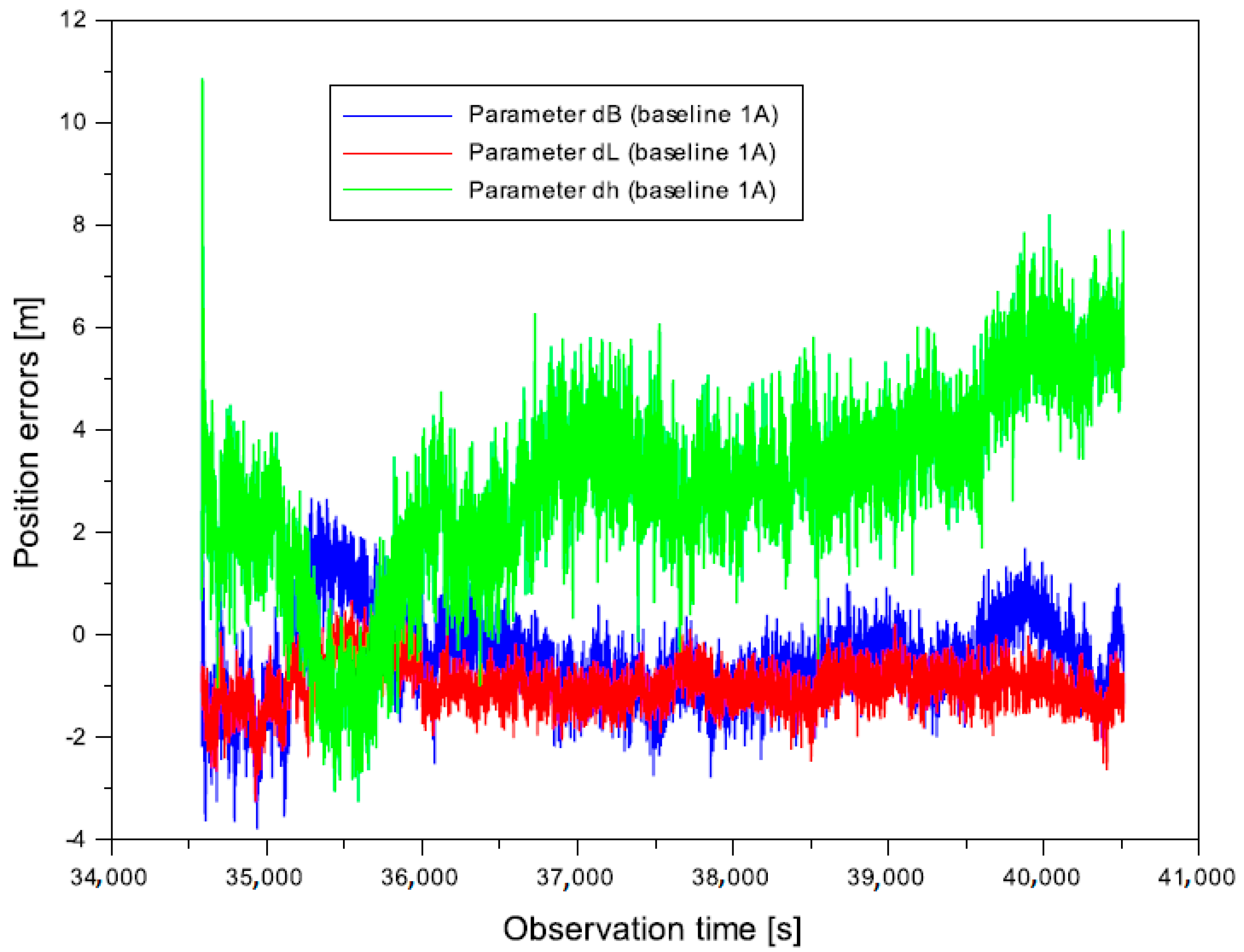
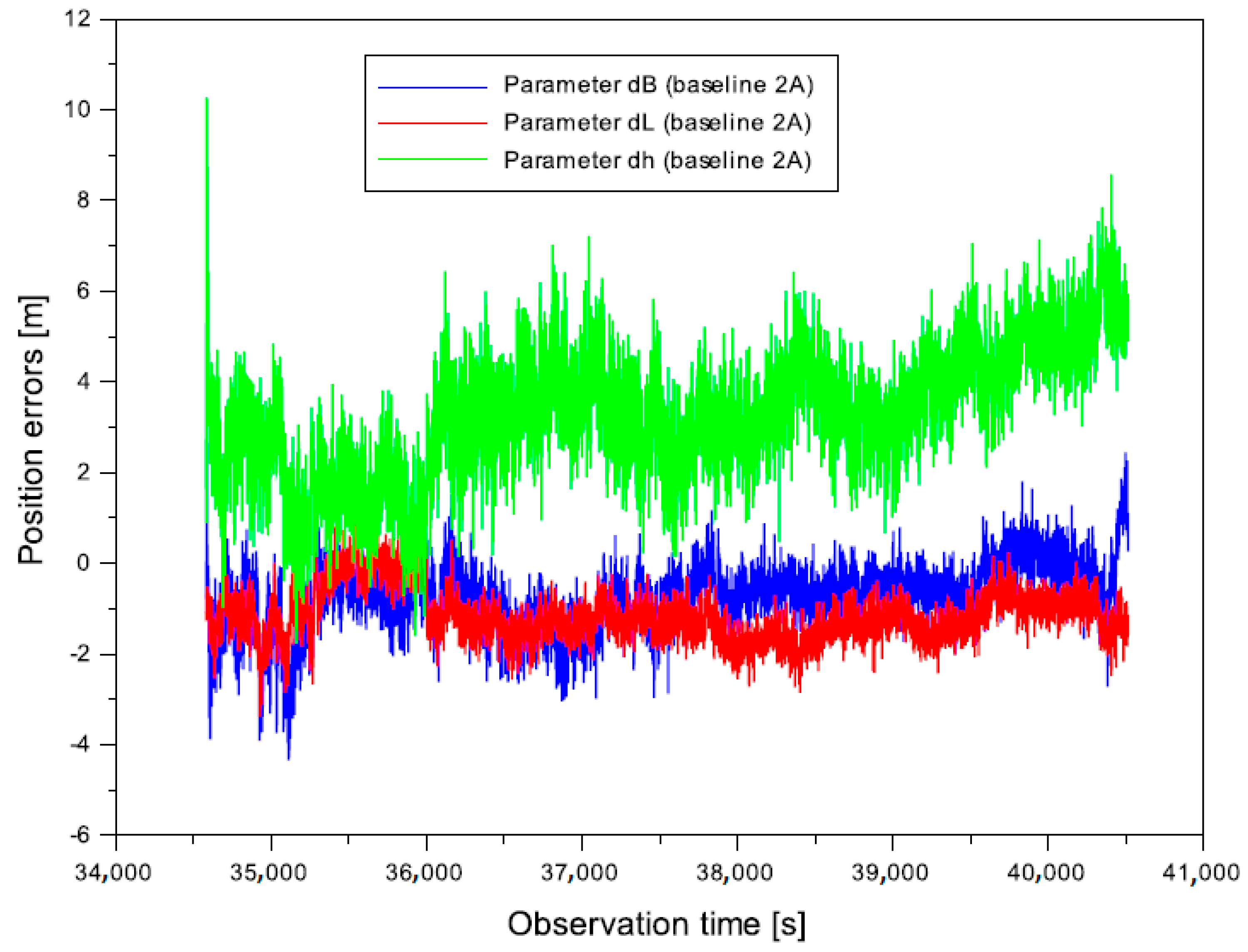
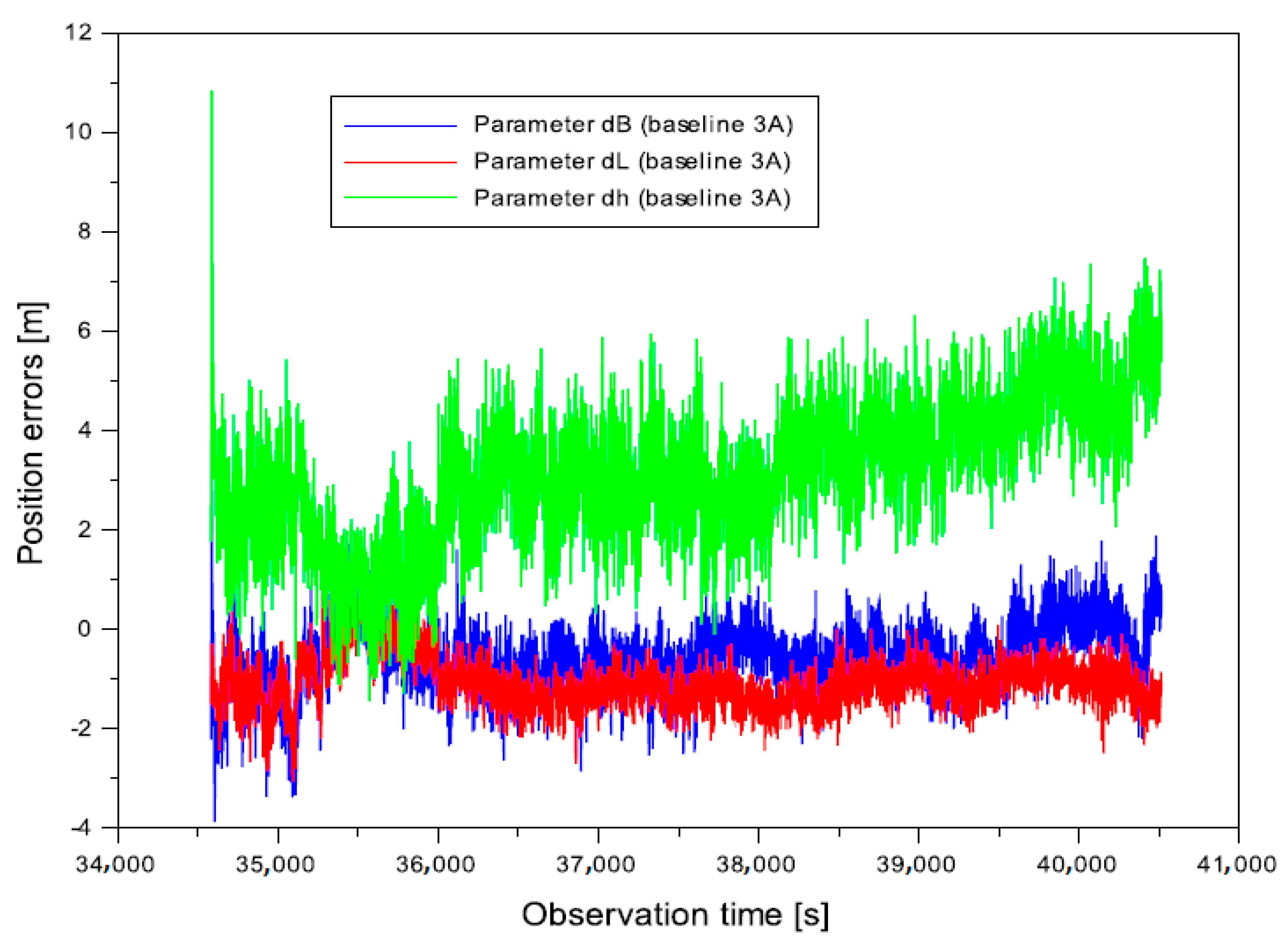
5. Results
- -
- from −0.482 to 4.988 m for the baseline ;
- -
- from −0.750 to 5.286 m for the baseline ;
- -
- from −0.565 to 3.797 m for the baseline .
- -
- from −0.993 to 0.677 m for the baseline ;
- -
- from −1.160 to 0.950 m for the base line ;
- -
- from −1.073 to 1.036 m for the baseline .
- -
- from −2.910 to 10.857 m for the baseline ;
- -
- from −3.296 to 10.269 m for the base line ;
- -
- from −3.151 to 10.846 m for the base line .
- -
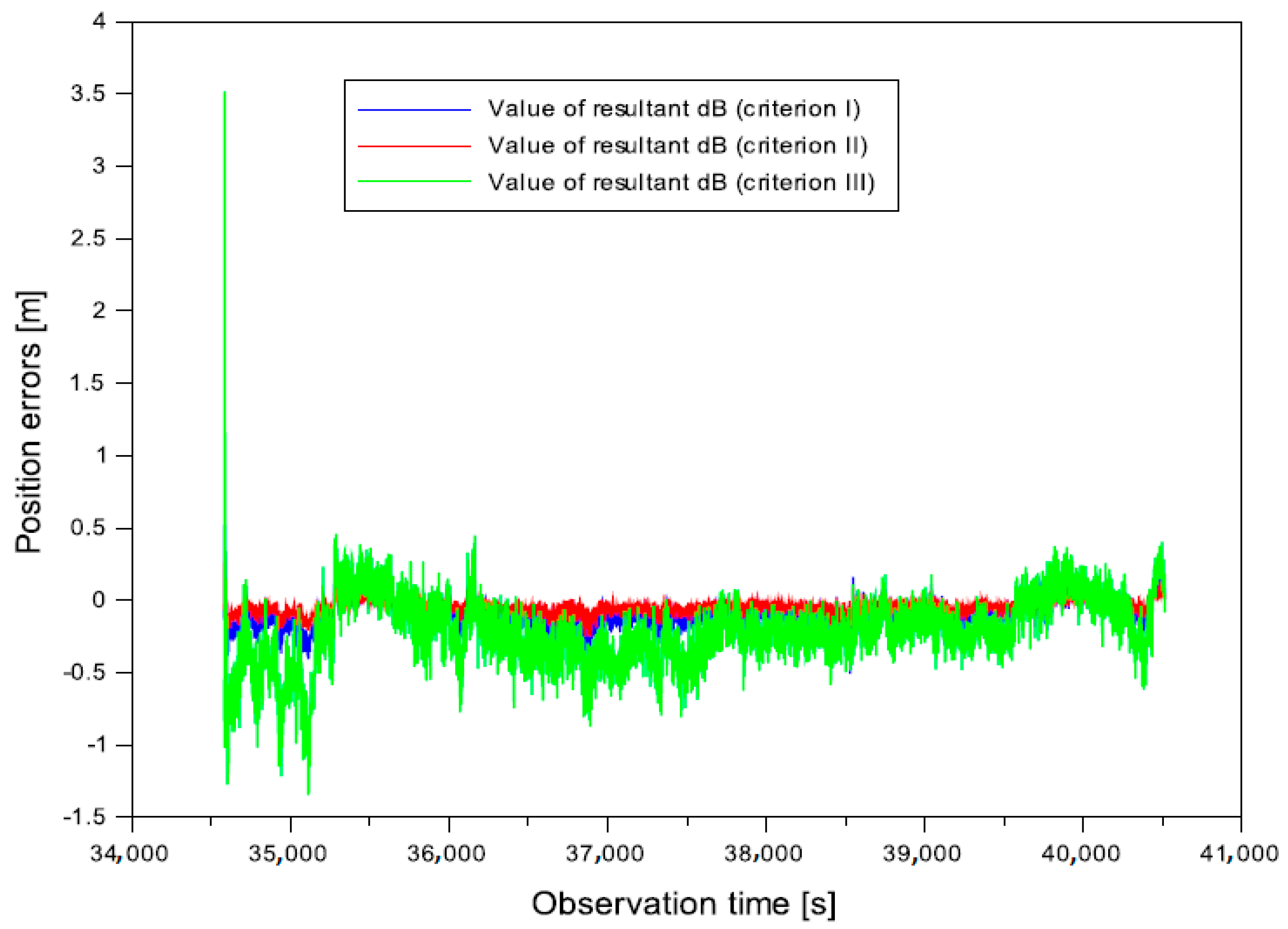
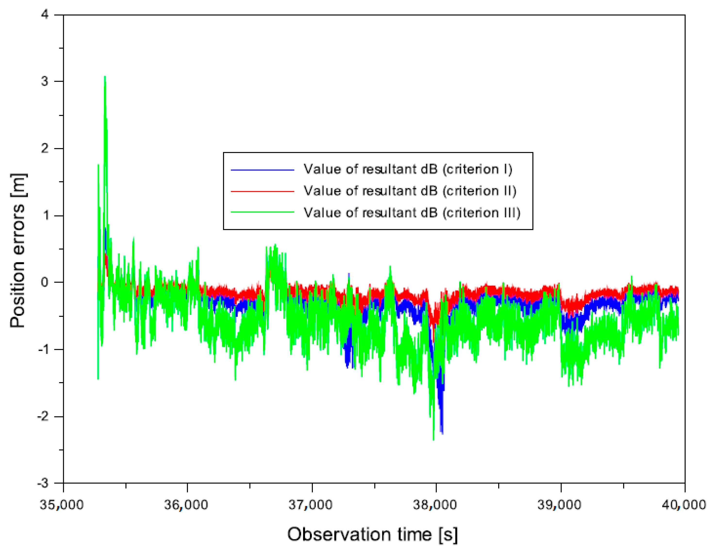
- from −0.508 to 0.519 m for the weighting in criterion I,
- -
- from −0.259 to 0.265 m for the weighting in criterion II,
- -
- from −1.346 to 3.518 m for the weighting in criterion III.
- -
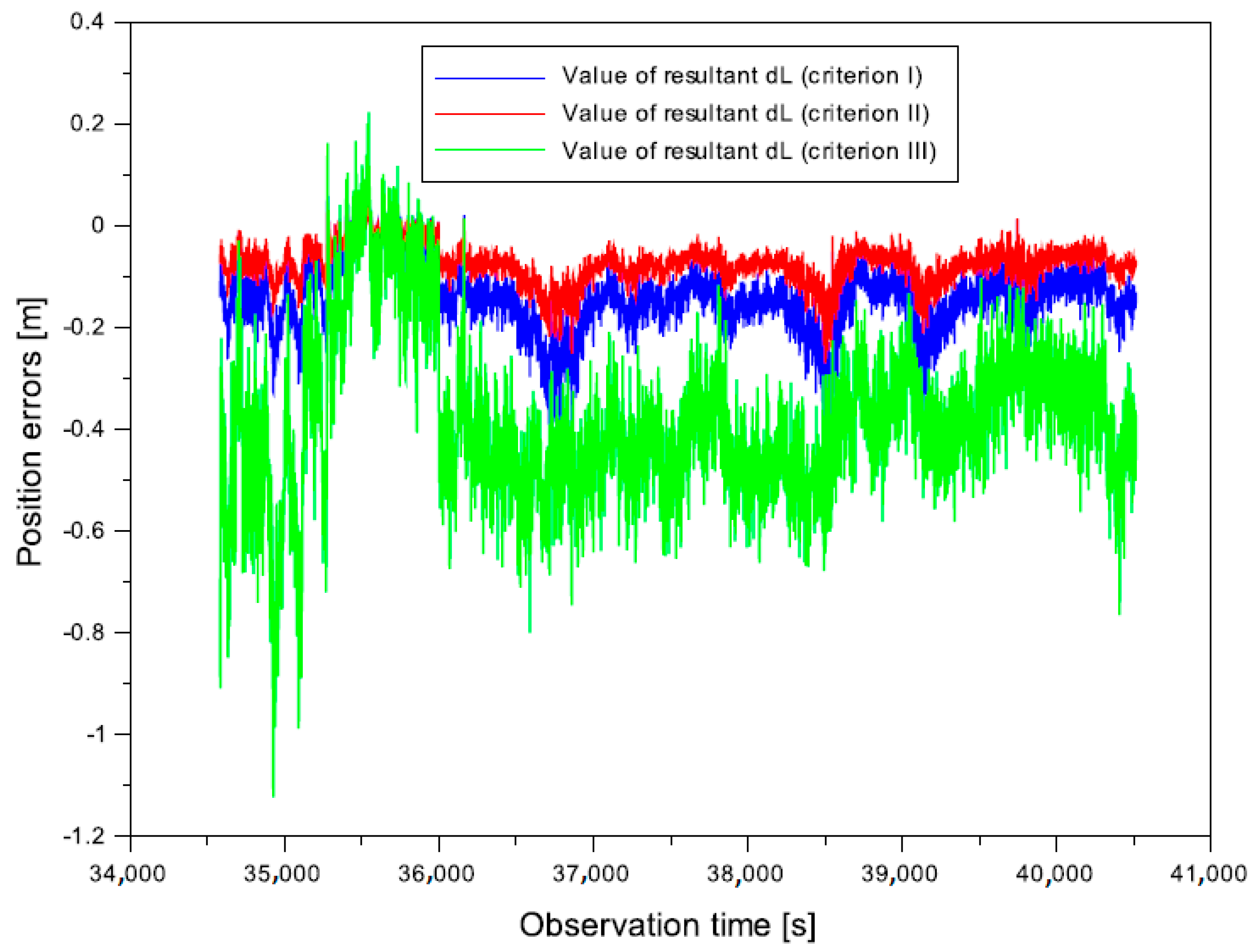
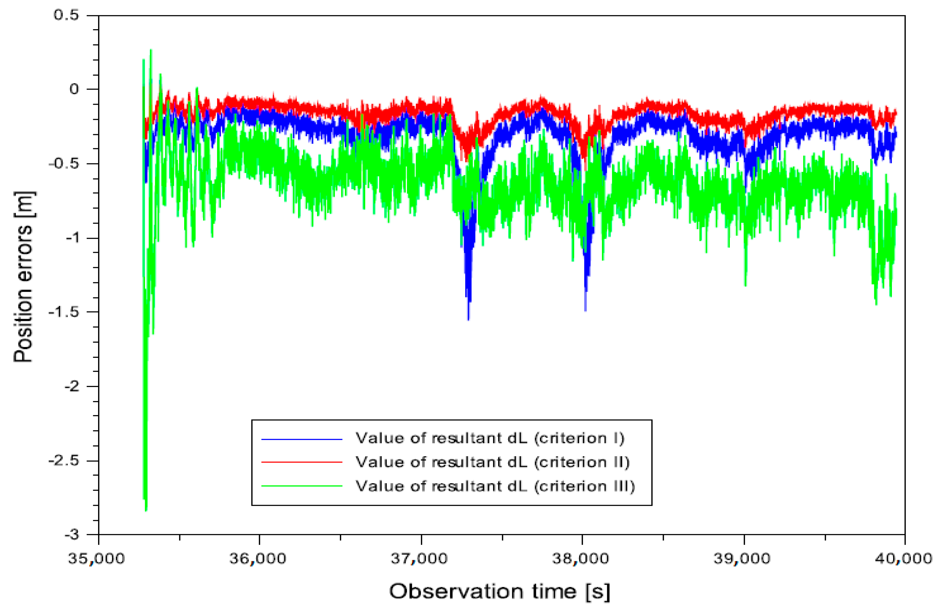
- from −0.488 to 0.091 m for the weighting in criterion I,
- -
- from −0.269 to 0.051 m for the weighting in criterion II,
- -
- from −1.122 to 0.223 m for the weighting in criterion III.
- -
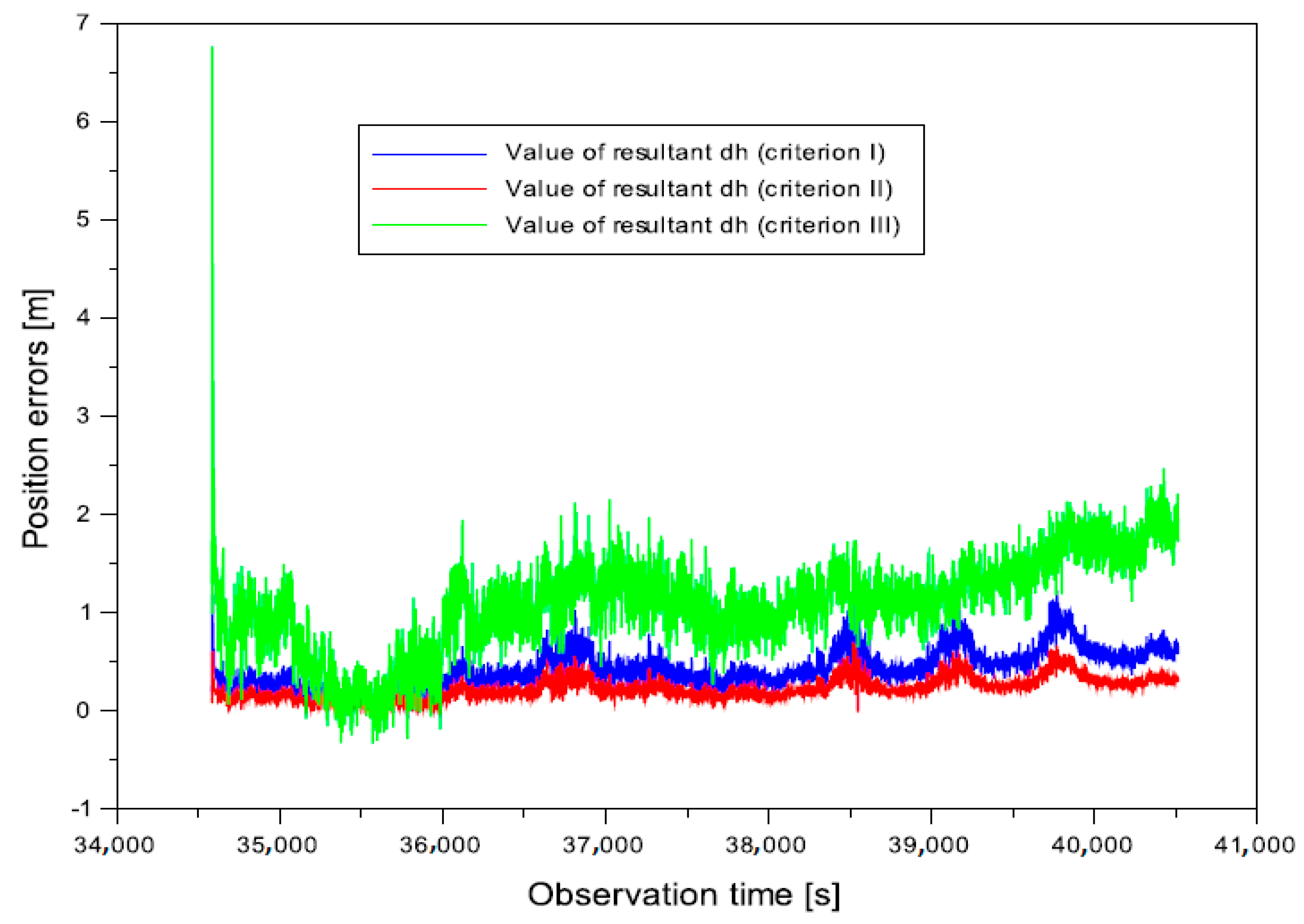
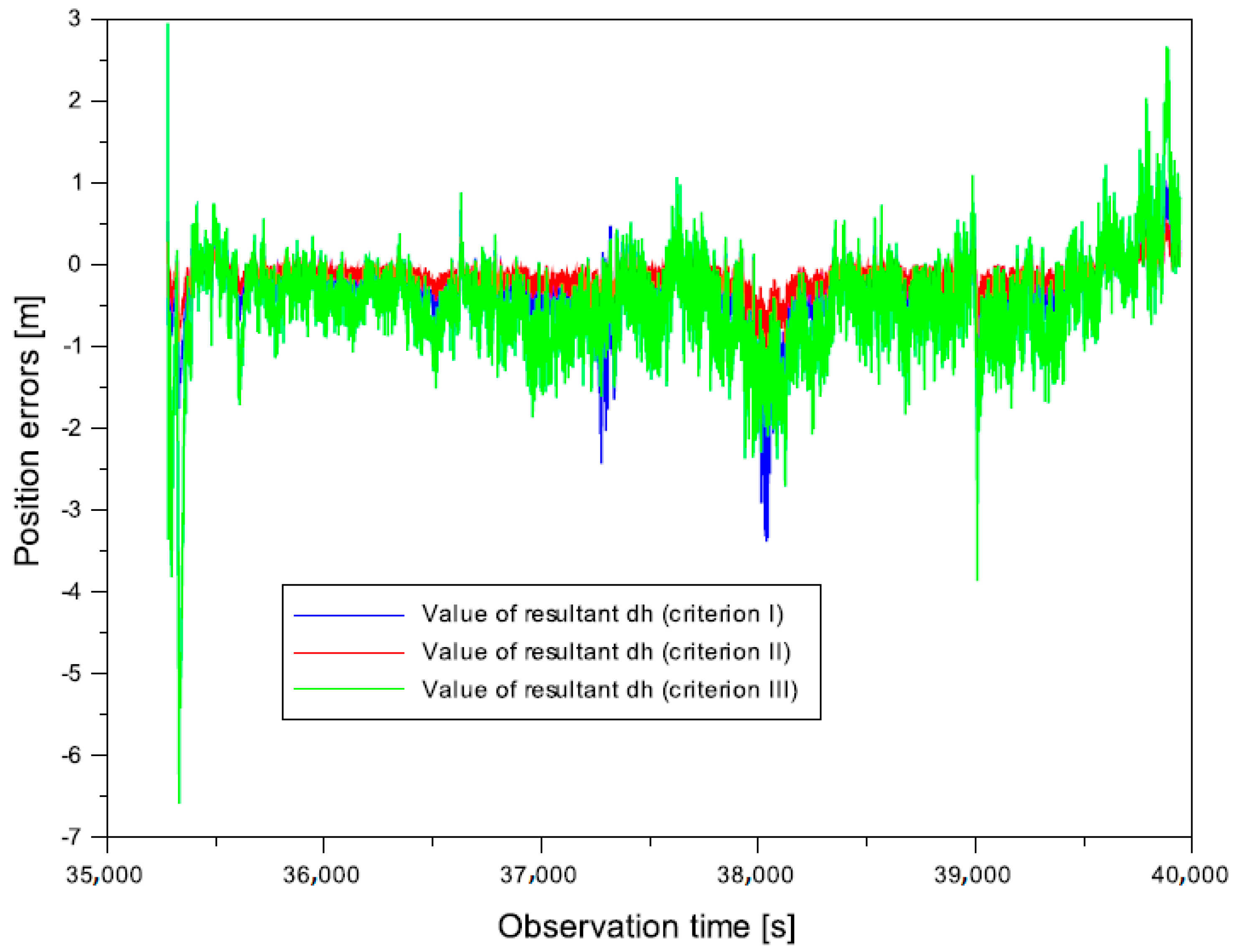
- from −0.078 to 1.334 m for the weighting in criterion I,
- -
- from −0.039 to 0.696 m for the weighting in criterion II,
- -
- from −0.332 to 6.764 m for the weighting in criterion III.
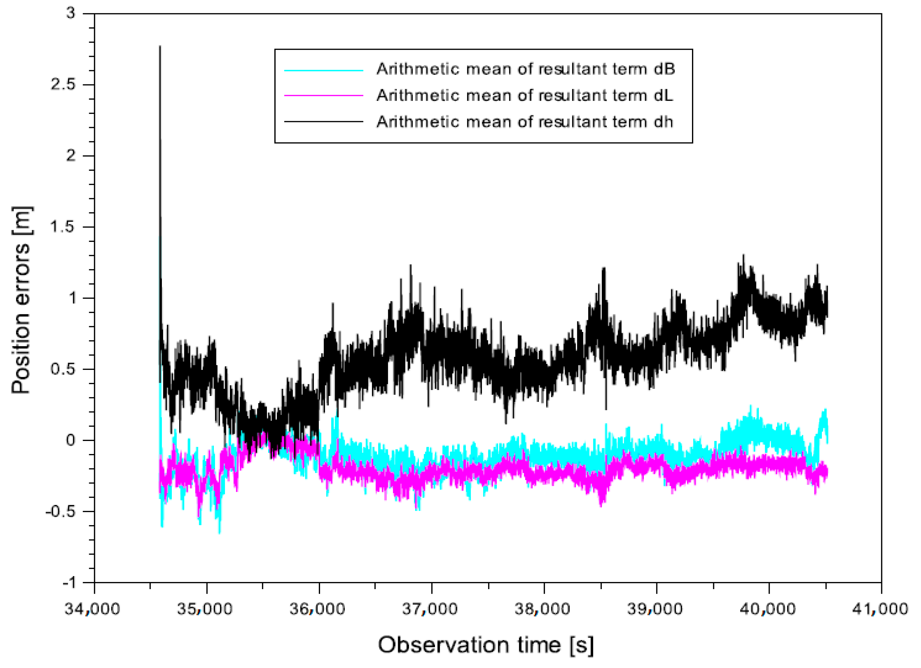
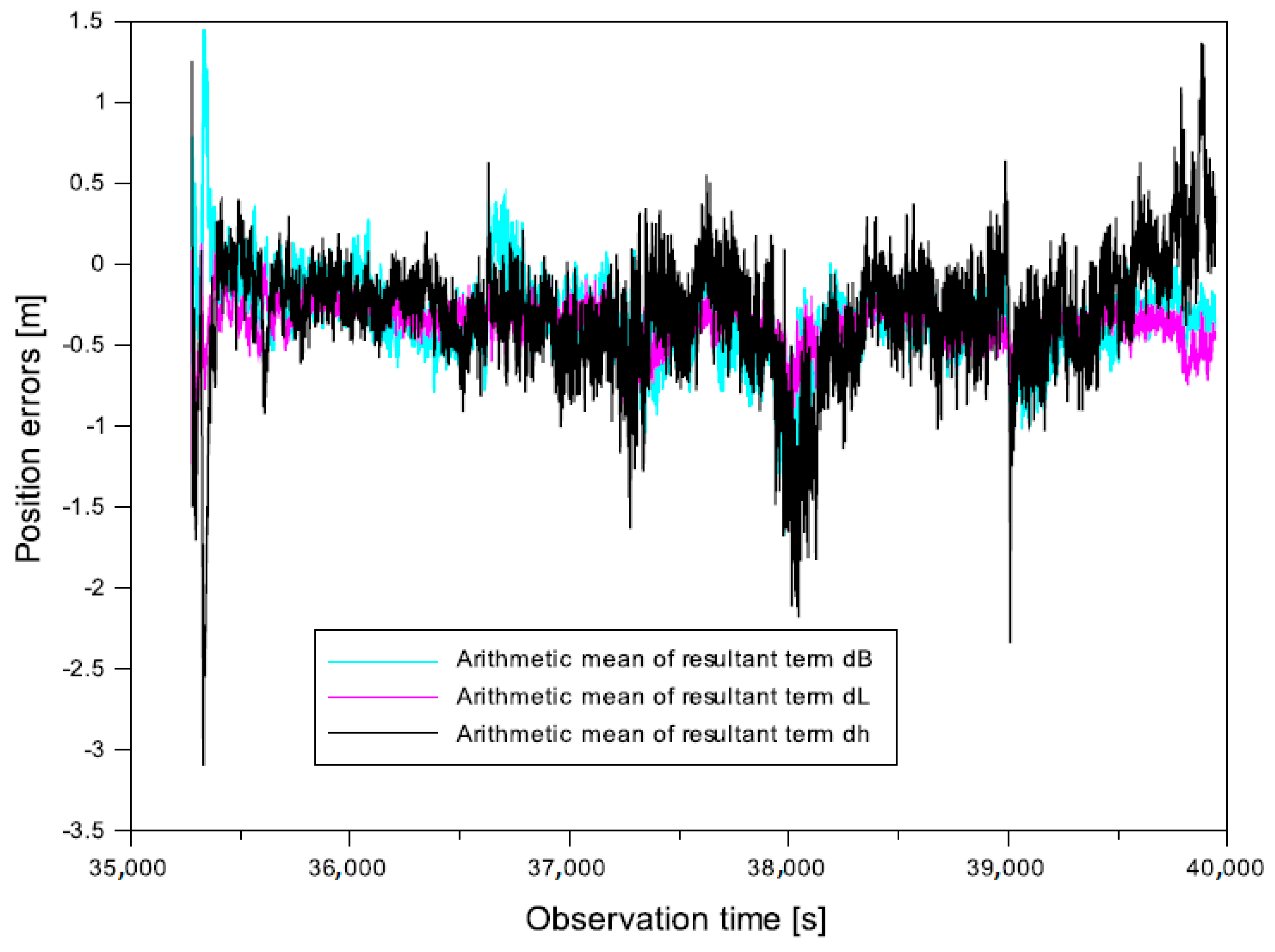
- —the arithmetic mean of the resultant position errors for criteria I–III,
- —the resultant position errors for coordinate B for criteria I–III,
- —the resultant position errors for coordinate L for criteria I–III,
- —the resultant position errors for coordinate h for criteria I–III.
- -
- from −0.114 to −0.654 m for the parameter ,
- -
- from −0.197 to −0.539 m for the parameter ,
- -
- from 0.575 to −0.146 m for the parameter .
6. Discussion
- -
- B = 51.816666667°, L = 21.866666666°, h = 150,000 m for VirA station;
- -
- B = 51.616666667°, L = 21.516666666°, h = 150,000 m for VirB station;
- -
- B = 51.46666666666°, L = 22.06666666667°, h = 150,000 m for VirC station.
- -
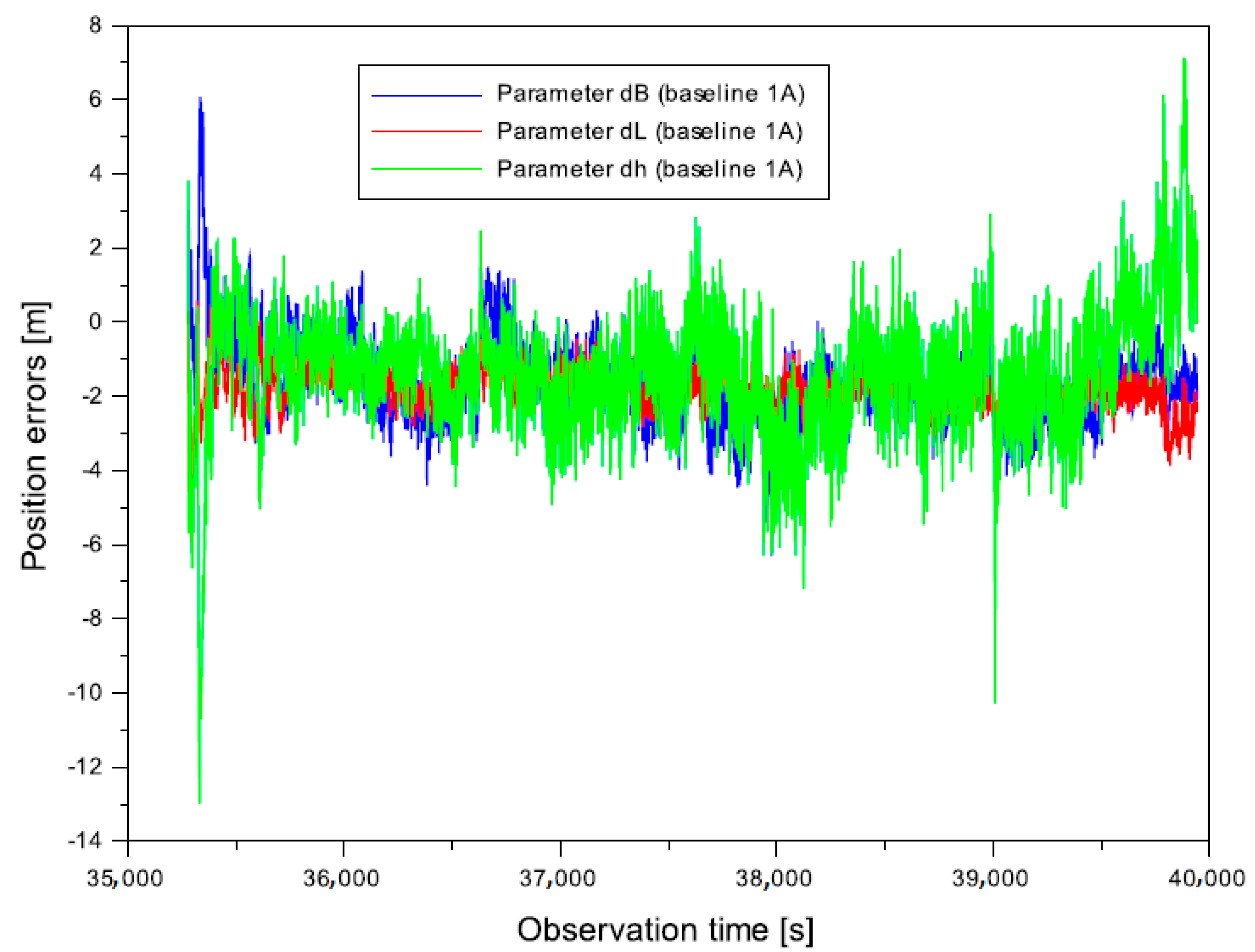
- from −6.302 to 6.075 m for the baseline ;
- -
- from −6.262 to 6.170 m for the baseline ;
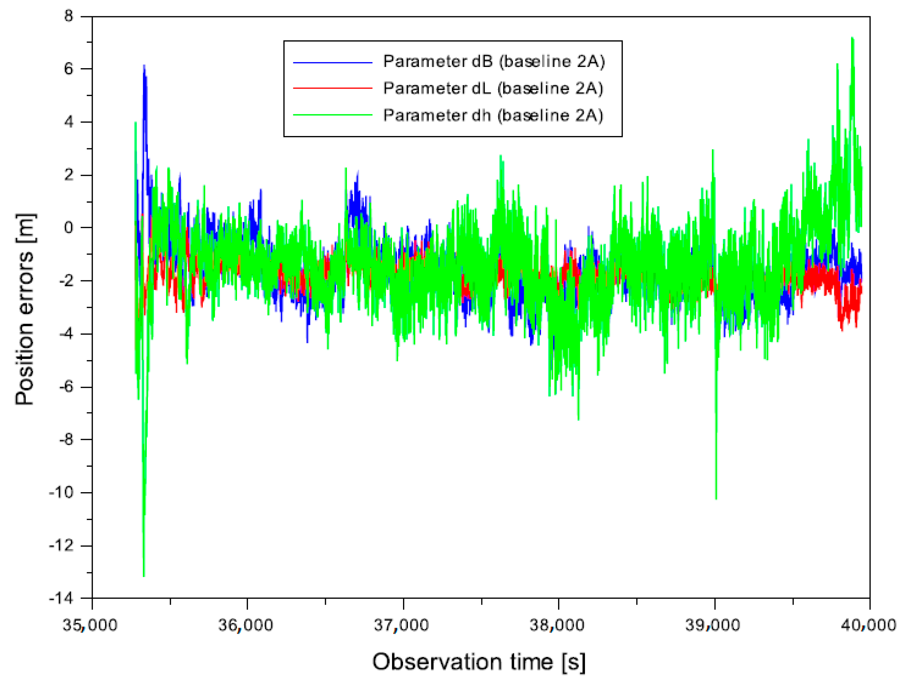
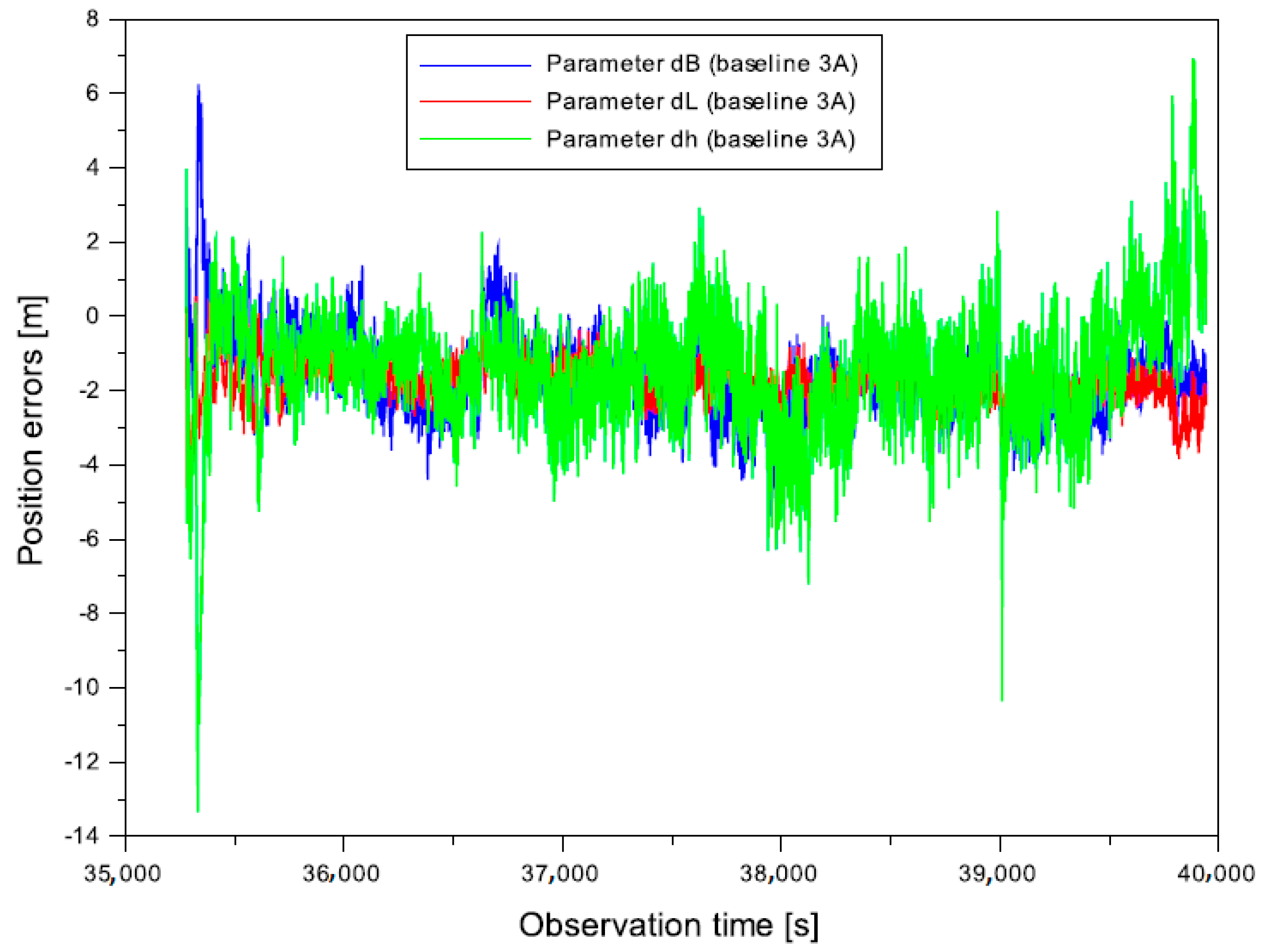
- -
- from −6.276 to 6.253 m for the baseline .
- -
- from −4.714 to 0.547 m for the baseline ;
- -
- from −4.746 to 0.542 m for the baseline ;
- -
- from −4.749 to 0.538 m for the baseline .
- -
- from −12.987 to 7.130 m for the baseline ;
- -
- from −13.175 to 7.208 m for the baseline ;
- -
- from −13.352 to 6.941 m for the baseline .
- -
- from 0.025 to 0.624 for the weight ,
- -
- from 0.025 to 0.245 for the weight ,
- -
- from 0.023 to 0.628 for the weight .
- -
- from 0.010 to 0.186 for the weight ,
- -
- from 0.010 to 0.127 for the weight ,
- -
- from 0.009 to 0.186 for the weight .
- -
- from 0.111 to 0.250 for the weight , , .
- -
- from −2.268 to 0.824 m for weighting criterion I,
- -
- from −0.901 to 0.440 m for weighting criterion II,
- -
- from −2.355 to 3.083 m for weighting criterion III.
- -
- from −1.556 to 0.072 m for weighting criterion I,
- -
- from −0.550 to 0.038 m for weighting criterion II,
- -
- from −2.842 to 0.271 m for weighting criterion III.
- -
- from −3.388 to 0.942 m for weighting criterion I,
- -
- from −1.137 to 0.502 m for weighting criterion II,
- -
- from −6.586 to 2.950 m for weighting criterion III.
- -
- from −1.679 to 1.449 m for the parameter ,
- -
- from −1.270 to 0.127 m for the parameter ,
- -
- from −3.095 to 1.368 m for the parameter .
7. Conclusions
- -
- in the case of the B component, there is a 55–94% error reduction;
- -
- for the L component, the improvement in positioning accuracy ranges from 62% to 94%;
- -
- for the ellipsoidal height h, the improvement in positioning accuracy ranges from 63% to 93%.
Author Contributions
Funding
Institutional Review Board Statement
Informed Consent Statement
Data Availability Statement
Acknowledgments
Conflicts of Interest
References
- Specht, M.; Szmagliński, J.; Specht, C.; Koc, W.; Wilk, A.; Czaplewski, K.; Karwowski, K.; Dąbrowski, P.; Chrostowski, P.; Grulkowski, S. Analysis of positioning methods using Global Navigation Satellite Systems (GNSS) in Polish State Railways (PKP). Sci. J. Marit. Univ. Szczecin 2020, 62, 26–35. [Google Scholar] [CrossRef]
- Mrozik, M.; Jafernik, H.; Krasuski, K. Methods of reduction of negative effects of exhaust emissions in airport area. In Contemporary Navigation, 2nd ed.; Ćwiklak, J., Ed.; Publisher of Military University of Aviation: Dęblin, Poland, 2020; Volume 2, pp. 271–282. (In Polish) [Google Scholar]
- Banaszek, K. Performance based navigation and GNSS/EGNOS system capabilities—Enabler for better positioning and separation of aircraft and airport capacity improvements. Logistyka 2010, 4, 1–9. [Google Scholar]
- Krasuski, K.; Ciećko, A.; Bakuła, M.; Wierzbicki, D. New strategy for improving the accuracy of aircraft positioning based on GPS SPP solution. Sensors 2020, 20, 4921. [Google Scholar] [CrossRef]
- Bakuła, M.; Uradziński, M.; Krasuski, K. Network code DGNSS positioning for faster L1-L5 GPS ambiguity initialization. Sensors 2020, 20, 5671. [Google Scholar] [CrossRef] [PubMed]
- Grzegorzewski, M. Navigating an aircraft by means of a position potential in three dimensional space. Annu. Navig. 2005, 9, 1–111. [Google Scholar]
- Krasuski, K.; Ćwiklak, J.; Cur, K. Determination of the precise trajectory of an aircraft flight in aviation experiments in Poland. In Contemporary Navigation, 1st ed.; Ćwiklak, J., Ed.; Publisher of Military University of Aviation: Dęblin, Poland, 2019; Volume 1, pp. 87–97. (In Polish) [Google Scholar]
- Krasuski, K.; Ćwiklak, J. Application of the DGPS method for the precise positioning of an aircraft in air transport. Sci. J. Sil. Univ. Technol. Ser. Transp. 2018, 98, 65–79. [Google Scholar] [CrossRef]
- Hofmann-Wellenhof, B.; Lichtenegger, H.; Wasle, E. GNSS—Global Navigation Satellite Systems: GPS, GLONASS, Galileo, and more; Springer: Vienna, Austria; New York, NY, USA, 2008; ISBN 978-3-211-73012-6. [Google Scholar]
- Przestrzelski, P.; Bakuła, M. Performance of real-time network code DGPS services of ASG-EUPOS in north-eastern Poland. Tech. Sci. 2014, 17, 191–207. [Google Scholar]
- Ciećko, A.; Bakuła, M.; Grunwald, G.; Ćwiklak, J. Examination of multi-receiver GPS/EGNOS positioning with Kalman filtering and validation based on CORS stations. Sensors 2020, 20, 2732. [Google Scholar] [CrossRef]
- Hothem, L.D.; Aiken, C.L.V.; Balde, M. Assessment of DGPS-derived aircraft trajectories by comparison with continuous kinematic GPS positioning. In Proceedings of the 5th International Technical Meeting of the Satellite Division of the Institute of Navigation (ION GPS 1992), Albuquerque, NM, USA, 16–18 September 1992; pp. 1079–1090. [Google Scholar]
- Grzegorzewski, M.; Jaruszewski, W.; Fellner, A.; Oszczak, S.; Wasilewski, A.; Rzepecka, Z.; Kapcia, J.; Popławski, T. Preliminary results of DGPS/DGLONASS aircraft positioning in flight approaches and landings. Annu. Navig. 1999, 1, 41–53. [Google Scholar]
- Lachapelle, G.; Cannon, M.E.; Qiu, W.; Varner, C. An analysis of differential and absolute GPS aircraft positioning. In Proceedings of the 1995 National Technical Meeting of The Institute of Navigation, Anaheim, CA, USA, 18–20 January 1995; pp. 701–710. [Google Scholar]
- Lachapelle, G.; Cannon, M.E.; Qiu, W.; Varner, C. Precise aircraft single-point positioning using GPS post-mission orbits and satellite clock corrections. J. Geod. 1996, 70, 562–571. [Google Scholar] [CrossRef]
- Tsai, Y.-J. Wide Area Differential Operation of the Global Positioning System: Ephemeris and Clock Algorithms. Ph.D. Thesis, Stanford University, Stanford, CA, USA, 1999; pp. 110–112. [Google Scholar]
- Tajima, H.; Asakura, M. Flight experiments of DGPS approaches and landings on a megafloat airport model. Trans. Jpn. Soc. Aeronaut. Space Sci. 2002, 45, 66–68. [Google Scholar] [CrossRef]
- Petrovska, O.; Rechkoska Shikoska, U. Aircraft precision landing using integrated GPS/INS system. Transp. Probl. 2013, 8, 17–25. [Google Scholar]
- Feit, C.; Bates, M. DGNSS positioning techniques for flight inspection. In Proceedings of the 4th International Conference on Differential Satellite Navigation Systems, DSNS-95, Bergen, Norway, 24–28 April 1995; pp. 1–8. [Google Scholar]
- Pervan, B.; Chan, F.-C.; Gebre-Egziabher, D.; Pullen, S.; Enge, P.; Colby, G. Performance analysis of carrier-phase DGPS navigation for shipboard landing of aircraft. NAVIG. J. Inst. Navig. 2003, 50, 181–192. [Google Scholar] [CrossRef]
- Günter, W.H.; Eissfeller, B.; Werner, W.; Ott, B.; Elrod, B.D.; Barltrop, K.; Stafford, J. Practical investigations on DGPS for aircraft precision approaches augmented by pseudolite carrier phase tracking. In Proceedings of the 10th International Technical Meeting of the Satellite Division of The Institute of Navigation (ION GPS 1997), Kansas City, MO, USA, 16–19 September 1997; pp. 1851–1860. [Google Scholar]
- Kee, C.; Park, S.; Yun, Y. Comparative study between GBAS and conventional aircraft precision approach guidance system. Trans. Jpn. Soc. Aeronaut. Space Sci. 2004, 46, 224–229. [Google Scholar] [CrossRef]
- Jia, H.; Dou, X.; Yuan, J. DGPS-based aircraft flight guidance/test system. IEEE Aerosp. Electron. Syst. Mag. 1996, 11, 23–26. [Google Scholar] [CrossRef]
- Hundley, W.; Rowson, S.; Courtney, G.; Wullschleger, V.; Velez, R.; O’Donnel, P. Flight evaluation of a basic C/A-code differential GPS landing system for category I precision approach. J. Inst. Navig. 1993, 40, 161–178. [Google Scholar] [CrossRef]
- Tortosa, D.; Beach, P. Accuracy and Precision Tests Using Differential GPS for NATURAL RESOURCE Applications; NODA Notes 18; Natural Resources Canada, Canadian Forest Service, Great Lakes Forestry Centre: Sault Ste. Marie, ON, Canada, 1996; pp. 1–10. [Google Scholar]
- Wormley, S.J. Application of Differential Global Positioning System (DGPS) indexing to remote sensing photogrammetry. In Review of Progress in Quantitative Nondestructive Evaluation. Review of Progress in Quantitative Nondestructive Evaluation; Thompson, D.O., Chimenti, D.E., Eds.; Springer: Boston, MA, USA, 1999; Volume 18, pp. 2109–2113. [Google Scholar] [CrossRef] [Green Version]
- Bruton, A.M.; Mostafa, M.M.R.; Scherzinger, B.M. Airborne DGPS without dedicated base stations for mapping applications. In Proceedings of the ION-GPS 2001, Salt Lake City, UT, USA, 11–14 September 2001. [Google Scholar]
- Mostafa, M.M.R. Precise airborne GPS positioning alternatives for the aerial mapping practice. In Proceedings of the FIG Working Week 2005 and GSDI-8, Cairo, Egypt, 16–21 April 2005; pp. 1–9. [Google Scholar]
- Ko, P.-Y. GPS-Based Precision Approach and Landing Navigation: Emphasis on Inertial and Pseudolite Augmentation and Differential Ionosphere Effect. Ph.D. Thesis, Stanford University, Stanford, CA, USA, 2000. [Google Scholar]
- Eggleston, B.; McKinney, W.D.; Choi, N.S.; Min, D. A low cost flight test instrumentation package for flight airplanes. In Proceedings of the 23rd Congress of International Council of the Aeronautical Sciences, Toronto, ON, Canada, 8–13 September 2002. Paper ICAS 2002-5.2.2. [Google Scholar]
- Sabatini, R.; Palmerini, G.B. Differential Global Positioning System (DGPS) for Flight Testing, RTO AGARDograph 160 Flight Test Instrumentation Series—DGPS Performance Analysis; RTO/NATO: Neuilly-sur-Seine, France, 2008; Volume 21, Chapter 6; ISBN 978-92-837-0041-8. [Google Scholar]
- Baroni, L.; Kuga, H.K. Analysis of navigational algorithms for a real time differential GPS system. In Proceedings of the 18th International Congress of Mechanical Engineering, Ouro Preto, Brazil, 6–11 November 2005. [Google Scholar]
- Gianniou, M.; Groten, E. An advanced real-time algorithm for code and phase DGPS. In Proceedings of the DSNS’96 Conference, St. Petersburg, Russia, 20–24 May 1996. [Google Scholar]
- Krasuski, K.; Ćwiklak, J.; Grzesik, N. Accuracy assessment of aircraft positioning by using the DGLONASS method in GBAS system. J. KONBIN 2018, 45, 97–124. [Google Scholar] [CrossRef] [Green Version]
- Pereira, V.A.S.; Monico, J.F.G.; de Oliveira Camargo, P. Estimation and analysis of protection levels for precise approach at Rio de Janeiro international airport using real time σVIG for each GPS and GLONASS satellite. Bol. Ciênc. Geod. 2021, 27. [Google Scholar] [CrossRef]
- Krasuski, K.; Ćwiklak, J. Aircraft positioning using DGNSS technique for GPS and GLONASS data. Sens. Rev. 2020, 40, 559–575. [Google Scholar] [CrossRef]
- Ali, Q.; Montenegro, S. A Matlab implementation of differential GPS for low-cost GPS receivers. TransNav 2014, 8, 343–350. [Google Scholar] [CrossRef] [Green Version]
- Przestrzelski, P.; Bakuła, M.; Galas, R. The integrated use of GPS/GLONASS observations in network code differential positioning. GPS Solut. 2017, 21, 627–638. [Google Scholar] [CrossRef] [Green Version]
- Krasuski, K.; Ćwiklak, J. Accuracy analysis of aircraft position at departure phase using DGPS method. Acta Mech. Autom. 2020, 14, 36–43. [Google Scholar] [CrossRef]
- Ali, A.S.A. Low-Cost Sensors-Based Attitude Estimation for Pedestrian Navigation in GPS-Denied Environments. Reports Number 20387: 43–46. Ph.D. Thesis, University of Calgary, Calgary, AB, Canada, 2013. [Google Scholar] [CrossRef]
- Krasuski, K.; Savchuk, S. Accuracy assessment of aircraft positioning using the dual-frequency GPS code observations in aviation. Commun. Sci. Lett. Univ. Zilina 2020, 22, 23–30. [Google Scholar] [CrossRef] [Green Version]
- Krasuski, K.; Wierzbicki, D. Application of the SBAS/EGNOS corrections in UAV positioning. Energies 2021, 14, 739. [Google Scholar] [CrossRef]
- Specht, C.; Pawelski, J.; Smolarek, L.; Specht, M.; Dabrowski, P. Assessment of the positioning accuracy of DGPS and EGNOS systems in the bay of Gdansk using maritime dynamic measurements. J. Navig. 2019, 72, 575–587. [Google Scholar] [CrossRef] [Green Version]
- ASG-EUPOS Website. Available online: http://www.asgeupos.pl/ (accessed on 30 May 2021).
- Takasu, T. RTKLIB ver. 2.4.2 Manual, RTKLIB: An Open Source Program. Package for GNSS Positioning. 2013. Available online: http://www.rtklib.com/prog/manual_2.4.2.pdf (accessed on 30 May 2021).
- Scilab Website. Available online: https://www.scilab.org/ (accessed on 30 March 2021).
- Specht, C.; Mania, M.; Skóra, M.; Specht, M. Accuracy of the GPS positioning system in the context of increasing the number of satellites in the constellation. Pol. Marit. Res. 2015, 22, 9–14. [Google Scholar] [CrossRef] [Green Version]
- Cellmer, S. Theoretical minimum value of PDOP determination. Tech. Sci. 2004, 7, 123–130. [Google Scholar]
- Langley, R.B. Dilution of precision. GPS World 1999, 10, 52–59. [Google Scholar]
- Matsushita, T.; Tanaka, T.; Yonekawa, M. Improvement accuracy in measurement of long baseline DGPS. In Proceedings of the 2008 SICE Annual Conference, Tokyo, Japan, 20–22 August 2008; pp. 3504–3508. [Google Scholar] [CrossRef]
- Matsushita, T.; Tanaka, T. Improving measurement accuracy of long baseline differential GPS. SICE J. Control Meas. Syst. Integr. 2010, 3, 157–163. [Google Scholar] [CrossRef] [Green Version]


| Marker of GNSS Base Station | Latitude (B) | Longitude (L) | Ellipsoidal Height (h) |
|---|---|---|---|
| VirA () | 50°25′00″, 00000 | 20°35′00″, 00000 | 200,000 m |
| VirB () | 50°23′00″, 00000 | 21°43′00″, 00000 | 200,000 m |
| VirC () | 50°17′00″, 00000 | 21°09′00″, 00000 | 200,000 m |
| Parameter | Value | Relationship |
|---|---|---|
| 0.643 | ||
| 0.835 | ||
| 1.326 | ||
| 0.856 | ||
| 0.926 | ||
| 1.081 | ||
| 0.883 | ||
| 0.923 | ||
| 1.046 |
| Parameter | Percentage Value (%) | Criterion of Measurement Weights | Baseline |
|---|---|---|---|
| 83 | I | ||
| 89 | I | ||
| 86 | I | ||
| 91 | II | ||
| 94 | II | ||
| 92 | II | ||
| 55 | III | ||
| 71 | III | ||
| 62 | III | ||
| 86 | I | ||
| 88 | I | ||
| 87 | I | ||
| 92 | II | ||
| 94 | II | ||
| 93 | II | ||
| 62 | III | ||
| 67 | III | ||
| 64 | III | ||
| 86 | I | ||
| 87 | I | ||
| 87 | I | ||
| 92 | II | ||
| 93 | II | ||
| 93 | II | ||
| 63 | III | ||
| 67 | III | ||
| 65 | III |
| Parameter | Value | Relation |
|---|---|---|
| 1.029 | ||
| 1.004 | ||
| 0.975 | ||
| 1.001 | ||
| 1.029 | ||
| 1.029 | ||
| 0.976 | ||
| 0.957 | ||
| 0.989 |
| Parameter | Percentage Value (%) | Criterion of Measurement Weights | Baseline |
|---|---|---|---|
| 82 | I | ||
| 82 | I | ||
| 82 | I | ||
| 91 | II | ||
| 91 | II | ||
| 91 | II | ||
| 65 | III | ||
| 64 | III | ||
| 65 | III | ||
| 83 | I | ||
| 83 | I | ||
| 82 | I | ||
| 91 | II | ||
| 91 | II | ||
| 91 | II | ||
| 65 | III | ||
| 64 | III | ||
| 63 | III | ||
| 78 | I | ||
| 81 | I | ||
| 81 | I | ||
| 90 | II | ||
| 90 | II | ||
| 90 | II | ||
| 63 | III | ||
| 64 | III | ||
| 64 | III |
Publisher’s Note: MDPI stays neutral with regard to jurisdictional claims in published maps and institutional affiliations. |
© 2021 by the authors. Licensee MDPI, Basel, Switzerland. This article is an open access article distributed under the terms and conditions of the Creative Commons Attribution (CC BY) license (https://creativecommons.org/licenses/by/4.0/).
Share and Cite
Krasuski, K.; Popielarczyk, D.; Ciećko, A.; Ćwiklak, J. A New Strategy for Improving the Accuracy of Aircraft Positioning Using DGPS Technique in Aerial Navigation. Energies 2021, 14, 4431. https://doi.org/10.3390/en14154431
Krasuski K, Popielarczyk D, Ciećko A, Ćwiklak J. A New Strategy for Improving the Accuracy of Aircraft Positioning Using DGPS Technique in Aerial Navigation. Energies. 2021; 14(15):4431. https://doi.org/10.3390/en14154431
Chicago/Turabian StyleKrasuski, Kamil, Dariusz Popielarczyk, Adam Ciećko, and Janusz Ćwiklak. 2021. "A New Strategy for Improving the Accuracy of Aircraft Positioning Using DGPS Technique in Aerial Navigation" Energies 14, no. 15: 4431. https://doi.org/10.3390/en14154431