Supercritical CO₂ Binary Mixtures for Recompression Brayton s-CO₂ Power Cycles Coupled to Solar Thermal Energy Plants

Abstract

In this work, an evaluation and quantification of the impact of using mixtures based on supercritical carbon dioxide “s-CO₂” (s-CO₂/COS, s-CO₂/H₂S, s-CO₂/NH₃, s-CO₂/SO₂) are made as a working fluid in simple and complex recompression Brayton s-CO₂ power cycle configurations that have pressure drops in their components. These cycles are coupled with a solar thermal plant with parabolic-trough collector (PTC) technology. The methodology used in the calculation performance is to establish values of the heat recuperator total conductance (UA_total) between 5 and 25 MW/K. The main conclusion of this work is that the cycle’s efficiency has improved due to using s-CO₂ mixtures as working fluid; this is significant compared to the results obtained using the standard fluid (pure s-CO₂). Furthermore, a techno-economic analysis is carried out that compares each configuration’s costs using pure s-CO₂ and a mixture of s-CO₂/COS with a molar fraction (70/30), respectively, as working fluid where relevant results are obtained. These results show that the best configuration in terms of thermal efficiency and cost is the RCC-RH for pure sCO₂ with values of 41.25% and 2811 $/kWe, while for the mixture sCO₂/COS, the RCC-2RH configuration with values of 45.05% and 2621 $/kWe is optimal. Using the mixture costs 6.75% less than if it is used the standard fluid (s-CO₂).

1. Introduction

In response to the increase in electrical energy needs and climate change globally, solar energy has become the fundamental pillar of the renewable energy market. In this field, concentrated solar power plants (CSP) have increased market share [1,2]. Currently, in order to reduce costs and improve the economic viability of solar thermal energy power plants (STE), researchers have focused on increasing the operating temperature, testing new heat transfer fluids (HTF) and cycles of power, thereby increasing system efficiency.

In this sense, supercritical carbon dioxide (s-CO₂) Brayton power cycles have been identified as a suitable candidate for next-generation CSP (CSP Gen3) applications as they can operate at higher temperatures achieving increased thermodynamic performance [3,4,5]. Various configurations of the s-CO₂ Brayton cycles (simple, recompression, recompression with main compression intercooling and partial cooling) are currently under study [6,7,8,9,10]. In the work of [7], it was determined that the recompression cycle showed the best performance compared to other configurations, i.e., simple, pre-compression, and split expansion. Furthermore, several studies by [6,11,12] showed that the recompression, partial cooling, and intermediate cycles are the most efficient circuits and even more so when they have reheating.

In addition to the above, the need to improve efficiency and have a working fluid that adapts to these variable environments (high and low temperatures) in power plants highlights the importance of optimizing equipment designs and the inlet and operating conditions. This obstacle can be overcome by adding small amounts of a selected compound to the base fluid (s-CO₂), thus producing a mixture to relocate the critical point in a first case to increase the critical temperature, which allows condensation in climates of 50 °C and 60 °C, while in the second case it is to decrease the critical temperature. For these reasons, it is crucial to consider the use of mixtures with s-CO₂ as a working fluid and to analyze its effects on operating conditions, mainly efficiency [13,14].

Currently, research has focused mainly on making mixtures with other gases [15]. In this way, the critical point of s-CO₂ can be adjusted to change the lowest or highest operating condition of the Brayton cycle. The direction and range of the critical point of the supercritical CO₂ mixture depend on the added substance and its quantity (mole fraction). [13], in their study on the influence of mixtures, conclude that there are two groups: mixtures that decrease the critical temperature (s-CO₂/He, s-CO₂/Kr, s-CO₂/CH₄ y s-CO₂/C₂H₆) and mixtures that increase the critical temperature (s-CO₂/COS, s-CO₂/H₂S, s-CO₂/NH₃, s-CO₂/SO₂, s-CO₂/C₅H₁₀, s-CO₂/C₅H₁₂), among others. They also mention that mixtures in recompression Brayton cycles increase efficiency by 3 and 4% compared to standard fluid (s-CO₂). So far, several studies have been conducted to discuss the feasibility and performance of the CO₂-based supercritical mixtures power cycle [16,17,18,19]. Ref. [20] Justify the possible use of CO₂-based mixtures that provide an increase or decrease in the critical point. In the study of [14] Perform a review where they discuss the potentialities of mixed CO₂ as working fluids in Brayton power cycles. They mention that it has been shown that mixing CO₂-N₂O₄ and CO₂-TiCl₄ can increase efficiency above 49%, assuming an inlet temperature to the turbine equal to 700 °C, which achieves at the same time a reduction of the complexity and costs of the power block. Furthermore, Ref. [15] analyze seven mixtures with different mass fractions in Brayton recompression cycles to maximize cycle efficiency. The main conclusion of this study is that with the increase or decrease of the CO₂ mass fraction, the different mixtures show different variations in the cycle performance.

Heat recovery is essential in the thermal efficiency of s-CO₂ Brayton cycles, making heat exchangers of particular relevance [21]. These Brayton cycles favor the use of compact heat exchangers (CHE), such as the printed circuit heat exchanger. This type of exchanger is used in the Brayton cycles of CSP plants mainly as regenerators due to its high ratio between heat transfer area and volume and its suitability to work under very high temperature and pressure conditions.

Numerous studies have been developed related to the CFD analysis of compact heat exchangers. In [22] studied pressure drop correlations in microchannel heat exchangers (MCHE) with zigzag configurations and S-fins for supercritical CO₂ cycle nuclear reactors. In [23,24] different studies and CFD analyses of printed circuit heat exchanger (PCHE) are produced that emphasize the optimization of the design parameters and in a recent investigation. Of particular interest is the study by [25] since different mixtures based on s-CO₂ is proposed to move the critical point and thus improve supercritical compression. In this sense, the research line [13] will be used as a reference to analyze various performance parameters of the PCHE exchanger.

The objectives of this study are various. On the one hand, we aim to optimize the cycle design through an evaluation of the thermal efficiency and techno-economic analysis of the simple and complex recompression configurations of the Brayton s-CO₂ power cycle, taking into account the pressure drops in the heat exchangers; furthermore, we aim to compare the benefits of the s-CO₂ mixtures (s-CO₂/COS, s-CO₂/H₂S, s-CO₂/NH₃, s-CO₂/SO₂) as working fluid, in these configurations coupled to concentrated solar energy (CSP) with parabolic trough collector technology (PTC). On the other hand, the study aims to achieve the simulation and modeling of a PCHE type heat exchanger for its application in Brayton s-CO₂ power cycles, as well as the validation of the results of the numerical analysis of ideal gas models, such as turbulence models, using CFD in PCHE regenerators that use pure supercritical carbon dioxide and s-CO₂-based mixtures that increase the critical temperature as a working fluid for comparative analysis and study of its behavior. Moreover, it seeks to analyze the impact on the heat exchange zone and, therefore, on the cycle’s economic efficiency, both of pure s-CO₂ and the different mixtures studied.

2. Materials and Methods

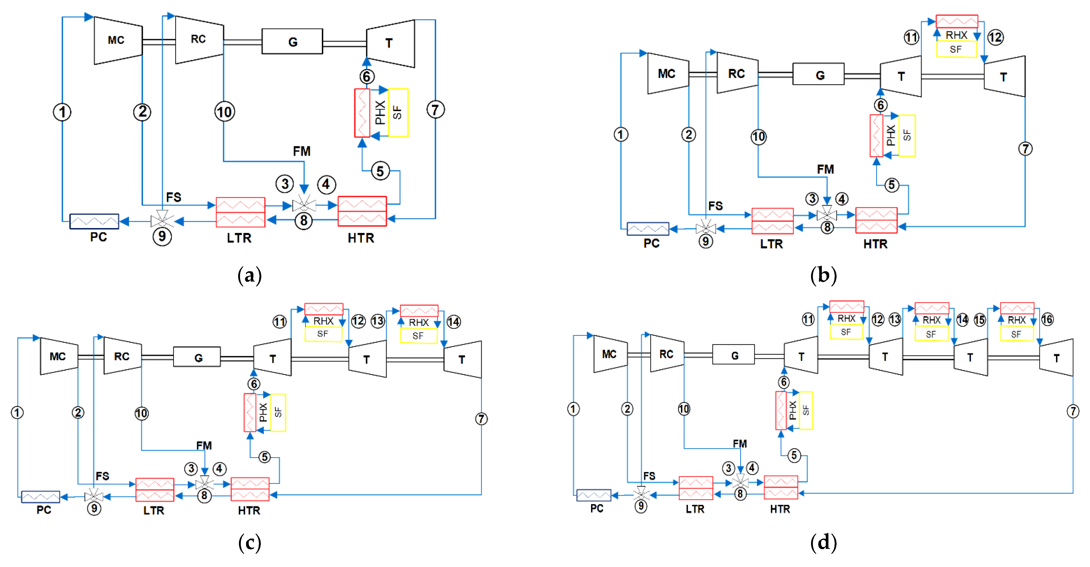
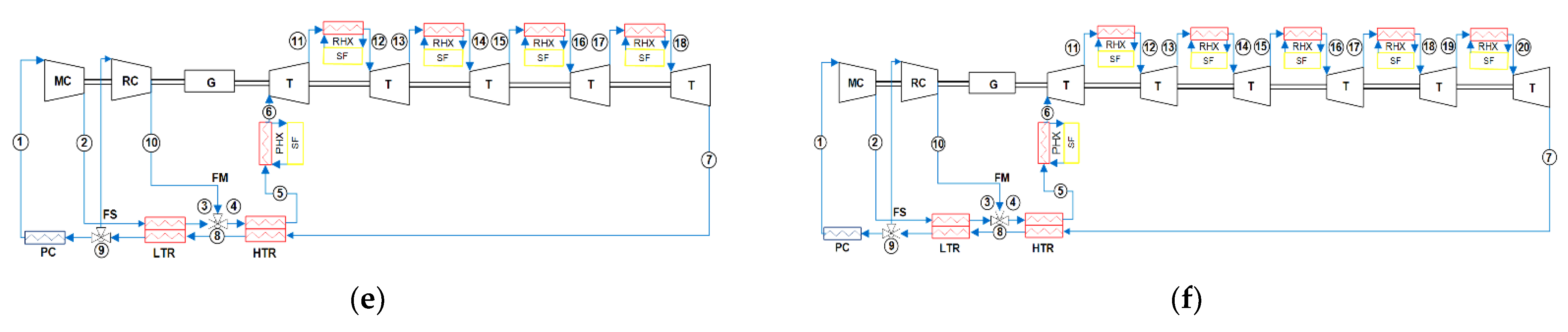
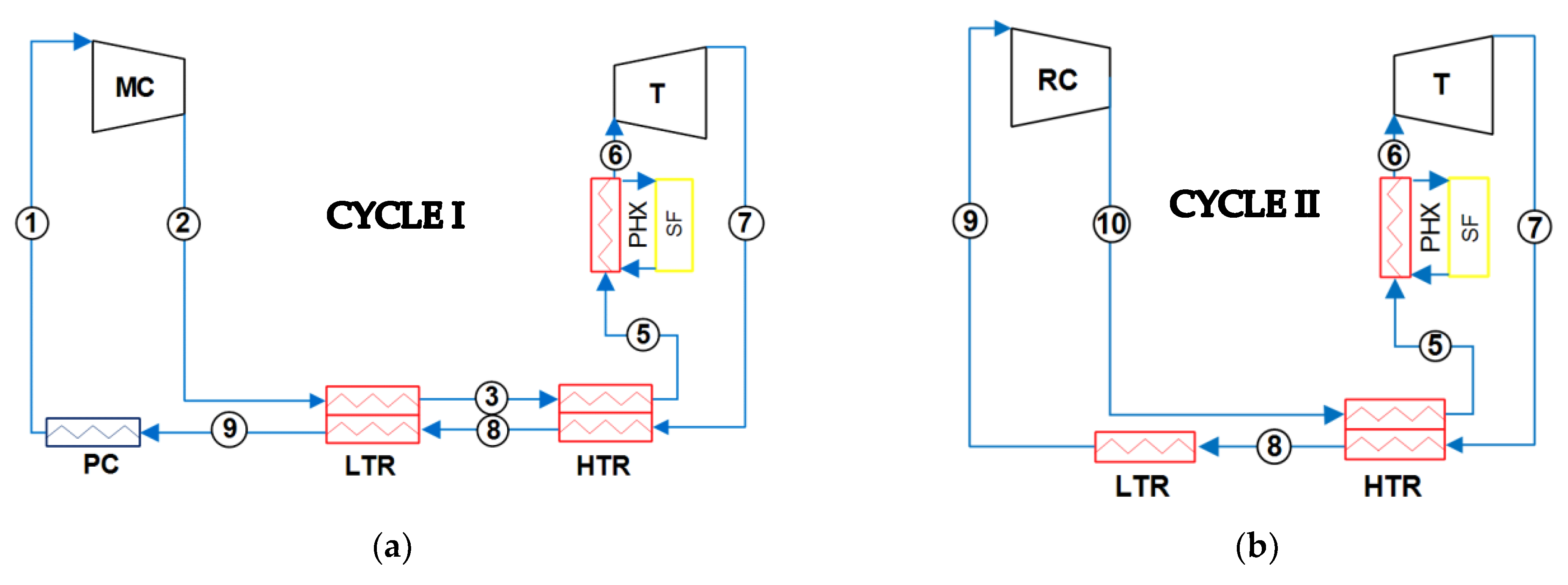
2.1. Cycles Layouts

The plant performance calculation sets a constant heat recuperator total conductance (UA) [26]. An inlet temperature to the compressor of 51 °C is established, as well as the pressure drops in the heat exchanger (PHX and RHXs), precooler (PC), and heat recuperators (LTR and HTR). In addition, some configurations of the Brayton cycle were studied: recompression (RCC), recompression with reheating (RCC-RH), and recompression with two reheatings (RCC-2RH); and complex configurations of the Brayton cycle were studied: recompression with three reheatings (RCC-3RH), recompression with four reheatings (RCC-4RH), and recompression with five reheatings (RCC-5RH).

The Software SCSP (Supercritical Concentrated Solar Power Plant) [26], that is based on the core of the software developed by [27] and and Thermoflex software [28] has been used for simulating the cycle configurations performance at design point (see Figure 1), operating as working fluid pure s-CO₂ and mixtures. The fluid’s properties were obtained from the REFPROP (Reference Fluid Properties) database developed by NIST (National Institute of Standards and Technology) in the USA [29]. Figure 2 shows the critical temperature distribution (a) and critical pressure (b) of the mixtures while varying the mole fraction of the added fluid. The first shows that the blends follow a nearly linear trend. Whereas, the second specifies that the pressure lines’ tendency is very different since there is a non-linearity between the critical pressure and the added mole fraction.

The main assumptions considered are summarized in

Table 1. Input parameters for mixtures increasing the critical temperature.

	Nomenclature	Value	Units
Net power output	W	50	MW
Compressor inlet temperature	T1	51	°C
Compressor inlet pressure	P1	optimized	MPa
Turbine inlet temperature	T6	550	°C
Turbine inlet pressure	P6	25	MPa
Compressor efficiency [12] and [30]	ηmc	0.89	-
Turbine efficiency [12] and [30]	ηt	0.93	-
UA for the low-temperature recuperator	UALT	2.5 to 12.5	MW/K
UA for the high-temperature recuperator	UAHT	2.5 to 12.5	MW/K
Split fraction (recompressor)	γ	optimized	-
Pressure drop for LTR and HTR	∆P/PLTR//∆P/PHTR	1.5//1.0	%
Pressure drop, precooler	∆P/PPC	2	%
Pressure drop for PHX and RHX	∆P/PPHX//∆P/PRHX	1.5//1.5	%

.

The thermal efficiency of these cycles compared to their recuperator total conductance using pure s-CO₂ as the working fluid without pressure drop in the components is shown in Figure 3.

The thermal efficiency of the recompression Brayton s-CO₂ cycle (Equations (1)–(6)) is appropriately defined as the net specific work divided by the net supply of heat. Thus, thermal efficiency can be expressed as:

$${\eta }_{th,RCC}=\frac{W_{T1}-\left(1-\gamma \right)\ast W_{MC}-\gamma \ast W_{RC}}{Q_{PHX}}$$

(1)

$${\eta }_{th,RCC\_RH}=\frac{W_{T1}+W_{T2}-\left(1-\gamma \right)\ast W_{MC}-\gamma \ast W_{RC}}{Q_{PHX}+Q_{RHX1}}$$

(2)

$${\eta }_{th,RCC\_2RH}=\frac{W_{T1}+W_{T2}+W_{T3}-\left(1-\gamma \right)\ast W_{MC}-\gamma \ast W_{RC}}{Q_{PHX}+Q_{RHX1}+Q_{RHX2}}$$

(3)

$${\eta }_{th,RCC\_3H}=\frac{W_{T1}+W_{T2}+W_{T3}+W_{T4}-\left(1-\gamma \right)\ast W_{MC}-\gamma \ast W_{RC}}{Q_{PHX}+Q_{RHX1}+Q_{RHX2}+Q_{RHX3}}$$

(4)

$${\eta }_{th,RCC\_4H}=\frac{W_{T1}+W_{T2}+W_{T3}+W_{T4}+W_{T5}-\left(1-\gamma \right)\ast W_{MC}-\gamma \ast W_{RC}}{Q_{PHX}+Q_{RHX1}+Q_{RHX2}+Q_{RHX3}+Q_{RHX4}}$$

(5)

$${\eta }_{th,RCC\_5H}=\frac{W_{T1}+W_{T2}+W_{T3}+W_{T4}+W_{T5}+W_{T6}-\left(1-\gamma \right)\ast W_{MC}-\gamma \ast W_{RC}}{Q_{PHX}+Q_{RHX1}+Q_{RHX2}+Q_{RHX3}+Q_{RHX4}+Q_{RHX5}}$$

(6)

where $W_T, W_{MC}, W_{RC}$ are the work done by the turbine, main compressor, and recompressor, respectively. $Q_{PHX}$ and $Q_{RHX}$ represent the solar field’s heat absorbed by the cycle through the primary heat exchanger and the reheat heat exchanger, respectively.

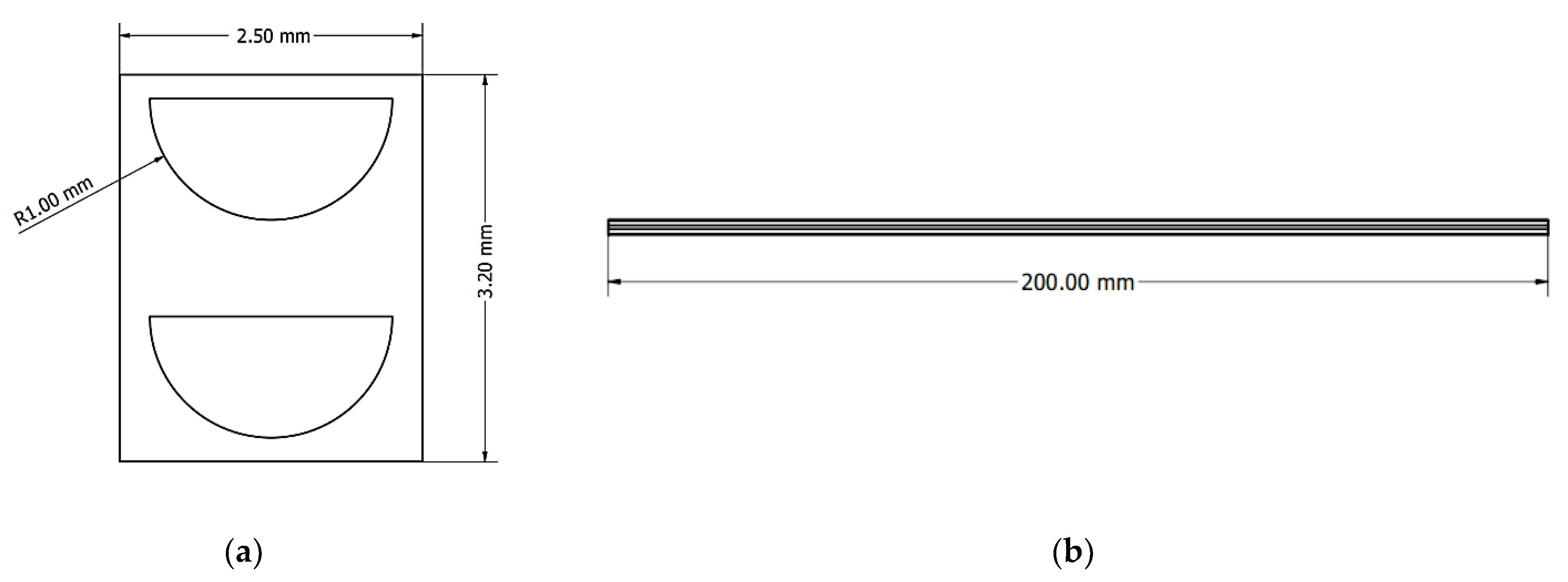
2.2. System Description PCHE

For the CFD simulation, the Ansys Fluent 2019 R2 software was used. Figure 4 shows the modeling of two PCHE exchange channels, a cold channel and a hot channel. The channels have a diameter of 2 mm and a maximum length of 200 mm. Due to its good behavior under high-temperature conditions and pressure, the Iconel 617 alloy was chosen as the material of the solid domain of the exchanger whose thermophysical properties are assumed constant—with a temperature of 298.7 K, the density is ($\mathsf{\rho }$) $8360\mathrm{kg}/{\mathrm{m}}^3$, the isobaric specific heat $(\mathrm{Cp})0.417\mathrm{kJ}/\mathrm{kg}·\mathrm{K}$, and the thermal conductivity $\left(\mathrm{k}\right)21\mathrm{W}/\mathrm{m}·\mathrm{K}.$

In

Table 2. Input parameters for mixtures increasing the critical temperature.

	Critical Temperature (K)	Critical Pressure (MPa)	Critical Density (kg/m3)
s-CO2 pure	304.13	7.3	467.6
s-CO2/COS (70/30)	324.15	7.815	467.139
s-CO2/H2S (60/40)	322.34	8.234	431.384
s-CO2/NH3 (81/19)	323.41	8.766	455.264
s-CO2/SO2 (90/10)	322.53	8.525	488.593

are listed the critical properties of the different mixtures.

The cold fluid properties were obtained for operating parameters of $T=400 \mathrm{K}$ and $P=22.5 \mathrm{M}\mathrm{P}\mathrm{a}$, while for the hot fluid, they are $T=630 \mathrm{K}$ and $P=9 \mathrm{M}\mathrm{P}\mathrm{a}$.

In order to validate the numerical model used, this study tried to emulate the results of the investigation carried out by [31] on CFD simulation of CO₂ supercritical in a PCHE. The reference study cited analyzes the behavior of pure supercritical carbon dioxide for different configurations of the printed circuit exchanger and different temperature ranges.

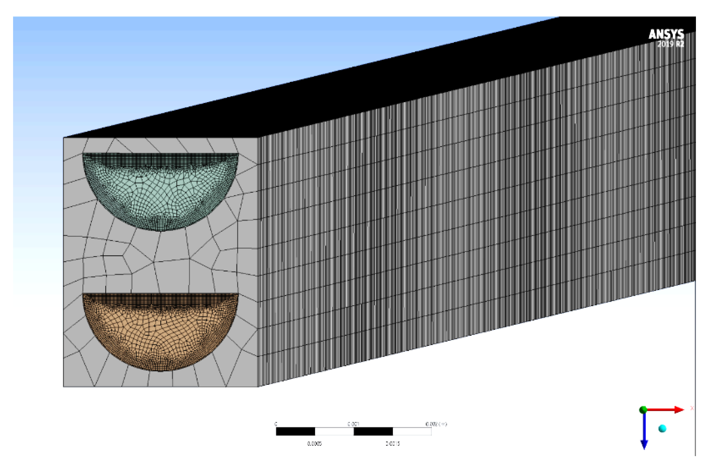
2.3. Mathematical Modeling for PCHE

To calculate fluid behavior in this study, we use the equation characteristics Equations (7)–(10). The value of i in the momentum equation represents equations in x, y, and z directions, and j is a summation index ranging from 1 to 3 [31].

Continuity equation:

$$\frac{\partial \left(\rho u_j\right)}{\partial x_j}=0$$

(7)

Momentum equation:

$$\rho \frac{\partial \left(u_i{u}_j\right)}{\partial x_j}=-\frac{\partial p_i}{\partial x_j}+\mu \frac{\partial }{\partial x_j}\left(\frac{\partial u_i}{\partial x_j}+\frac{\partial u_j}{\partial x_i}-\frac{2}{3}{\delta }_{ij}\frac{\partial u}{\partial x_k}\right)$$

(8)

Energy equation:

$$\frac{\partial }{\partial x_j}\left[u_j\left(\rho E+p\right)\right]=\frac{\partial }{\partial x_j}\left(\left(k_f+k_t\right)\frac{\partial T}{\partial x_j}\right)$$

(9)

The energy equation for the solid domain:

$$\frac{\partial }{\partial x_j}\left(k_s\frac{\partial T}{\partial x_j}\right)=0$$

(10)

where ${\delta }_{ij}$ is the Kronecker delta, $\rho$ represents fluid density (kg/m³), $p$ in the pressure (kPa), $u_j$ is the velocity component in j direction (m/s), $k_f$ represents thermal conductivity of solid (W/m-K), and $k_t$ is turbulent kinetic energy.

The turbulence model used in this study is the Reynolds-averaged Navier–Stokes (RANS) standard $k-\epsilon$ model with wall function. This model is the most common due to its low computational cost. However, for this model, it is required to solve two additional equations—Equations (11) and (12)—the equation for turbulent kinetic energy transport $\left(k\right)$ and the equation for the dissipation rate of turbulent kinetic energy $\left(\epsilon \right).$ The transport equations [32] of this model are shown below:

$$\frac{\partial }{\partial t}\left(\rho k\right)+\frac{\partial }{\partial x_i}\left(\rho k{u}_i\right)=\frac{\partial }{\partial x_j}\left(\left(\mu +\frac{{\mu }_t}{{\sigma }_k}\right)\frac{\partial k}{\partial x_j}\right)+G_k+G_b-\rho \epsilon -Y_M+S_k$$

(11)

$$\frac{\partial }{\partial t}\left(\rho \epsilon \right)+\frac{\partial }{\partial x_i}\left(\rho \epsilon u_i\right)=\frac{\partial }{\partial x_j}\left(\left(\mu +\frac{{\mu }_t}{{\sigma }_{\epsilon }}\right)\frac{\partial \epsilon }{\partial x_j}\right)+C_{1\epsilon }\frac{\epsilon }{k}\left(G_k+C_{3\epsilon }{G}_b\right)-C_{2\epsilon }\rho \frac{{\epsilon }^2}{k}+S_{\epsilon }$$

(12)

where ${\mu }_t$ is the turbulent viscosity, $G_k$ represents the generation of turbulence of kinetic energy due to velocity gradients, $G_b$ represents the generation of turbulence of kinetic energy due to buoyancy, and $Y_M$ is the contribution of fluctuating dilation to the total dissipation rate.

Due to the supercritical conditions of the fluids used in this work, it is not feasible to use a typical real gas model. For this reason, the model used in the numerical simulation is the Aungier–Redlich–Kwong real gas model [33]. This model is recommended for calculations with fluids and mixtures of fluids in vapor or supercritical state. Ansys Fluent has adopted this equation for improved accuracy, especially when we are near the critical point, as in this case.

$$P=\frac{RT}{V-b+c}-\frac{a\left(T\right)}{V\left(V+b\right)}$$

(13)

where the parameters involved are obtained from the following expressions [34]. The Aungier-Redlich-Kwong Model:

$$a\left(T\right)=a_0{T}_r^{-n}$$

(14)

$$c=\frac{R{T}_c}{P_c+\frac{a_0}{V_c\left(V_c+b\right)}}+b-V_c$$

(15)

$$n=0.4986+1.735\omega +0.475{\omega }^2$$

(16)

$$a_0=\frac{0.42747 R^2{T}_c^2}{P_c}$$

(17)

$$b=\frac{0.08664 R T_c}{P_c}$$

(18)

where $P_c$ ($\mathrm{P}\mathrm{a}$) is the critical pressure, $V_c$ (${\mathrm{m}}^3/\mathrm{k}\mathrm{g}$) is the critical specific volume, and $\omega$ is the acentric factor.

Mesh sensitivity analysis is fundamental in this work. A series of simulations are carried out in which the size of the mesh is varied by 5%. In this case, it was decided to alter the mesh size of the fluid domain, keeping the mesh of the solid material constant (see Figure 5). Furthermore, by modifying the mesh of the fluid domain, the size of the cell closest to the wall is also changed, which allows analyzing the results for different values of $y^{+}.$ To ensure the reliability of the mesh, the Richardson extrapolation of the results for the temperature profile was performed. Finally, a mesh dependency study to ensure the reliability of the results was carried out. Cell size was modified, emphasizing the $y^{+}$ value for this purpose. [35] Confirmed that for $k-\epsilon$ turbulence models such as the one used in the present case, wall functions are the most appropriate since this turbulence model is valid for regions where turbulence is fully developed. Adopting a wall function remains the most common solution among CFD approaches, as mentioned by [36]; and it also enables the mesh resolution required for a high Reynolds number to be reduced [37]. The cells adjacent to the wall are therefore placed in the logarithmic region $\left(y^{+}>32.5\right)$ to ensure the accuracy of the result. The expression that defines the wall function for the range of $y^{+}$ characteristic of this region is the following [38]:

$$y^{+}=\frac{y{u}_{\tau }}{v}$$

(19)

$${\mu }_T=\sqrt{\frac{{\tau }_w}{\rho }}$$

(20)

$$u^{+}=\frac{1}{k} ln\left(y^{+}\right)+B$$

(21)

where $y$ is the absolute distance from the wall, $u_{\tau }$ represents the so-called friction velocity, $\nu$ is the kinematic viscosity of the fluid, and ${\tau }_w$ represents the shear stress in the wall. The Von Karman constant is $k=0.41$ and the constant $B=5.2$, where $u^{+}=u/u_{\tau }$.

3. Results and Discussion

This section shows the results obtained in the different simulations and their comparison with the reference data of pure s-CO₂.

The plant’s gross efficiency is calculated by setting the total recuperator conductance for only inlet temperature in the turbines (T₆—Table 1). Then, the compressor inlet pressure and the recompression fraction are optimized with the mathematical algorithms SUBPLEX, UOBYQA, and NEWOUA [26].

The thermal efficiency of these cycles compared to their recuperator total conductance using pure s-CO₂ as the working fluid with pressure drop in the components is shown in Figure 6.

As shown in Figure 6, an increase in pressure drop has a detrimental effect on the thermal efficiency of the Brayton s-CO₂ cycle by reducing the gap between reheat and no-reheat configurations [39].

In most cases, the optimal efficiency is obtained when the working fluid’s critical point is close to the compressor inlet temperature (CIT). It can be observed that the mixtures that imply the best cycle efficiency are s-CO₂/COS (70/30) and s-CO₂/H₂S (60/40). These mixtures increase the cycle efficiency between 3 and 4 points (Figure 7a, Figure 8a, Figure 9a and Figure 10a). Whereas, the mixtures of s-CO₂/NH₃ and s-CO₂/SO₂ with molar fractions of (81/19) and (90/10), respectively, increase their efficiency between 2 and 3 points (Figure 7a, Figure 8a, Figure 9a and Figure 10a).

However, in Figure 11a and Figure 12a, the best cycle efficiency is obtained with the mixtures s-CO₂/COS (70/30) and s-CO₂/H₂S (60/40). These mixtures increase the cycle efficiency between 5 and 6 points. Whereas, the mixtures of s-CO₂/NH₃ and s-CO₂/SO₂ with molar fractions of (81/19) and (90/10), respectively, increase their efficiency between 3 and 4 points. Furthermore, the results indicate that as the number of reheats increases, the gap between the mixture’s efficiency with carbonyl sulfide and hydrogen sulfide widens.

The total recuperator conductance is directly related to the increase in cycle efficiency. However, this increase is limited by decreasing the “pinch point”, which can be defined as the minimum temperature difference between the hot and cold streams in each heat recuperator (LTR and HTR). The recuperators’ characteristic operating values are considered pinch point temperatures between 5–10 °C; however, these temperatures can be reduced to a range of 2–5 °C in the studied configurations [27]. Figure 7b, Figure 8b, Figure 9b, Figure 10b, Figure 11b and Figure 12b for RCC configurations show that the pinch point decreases by increasing the cycle’s UA_total.

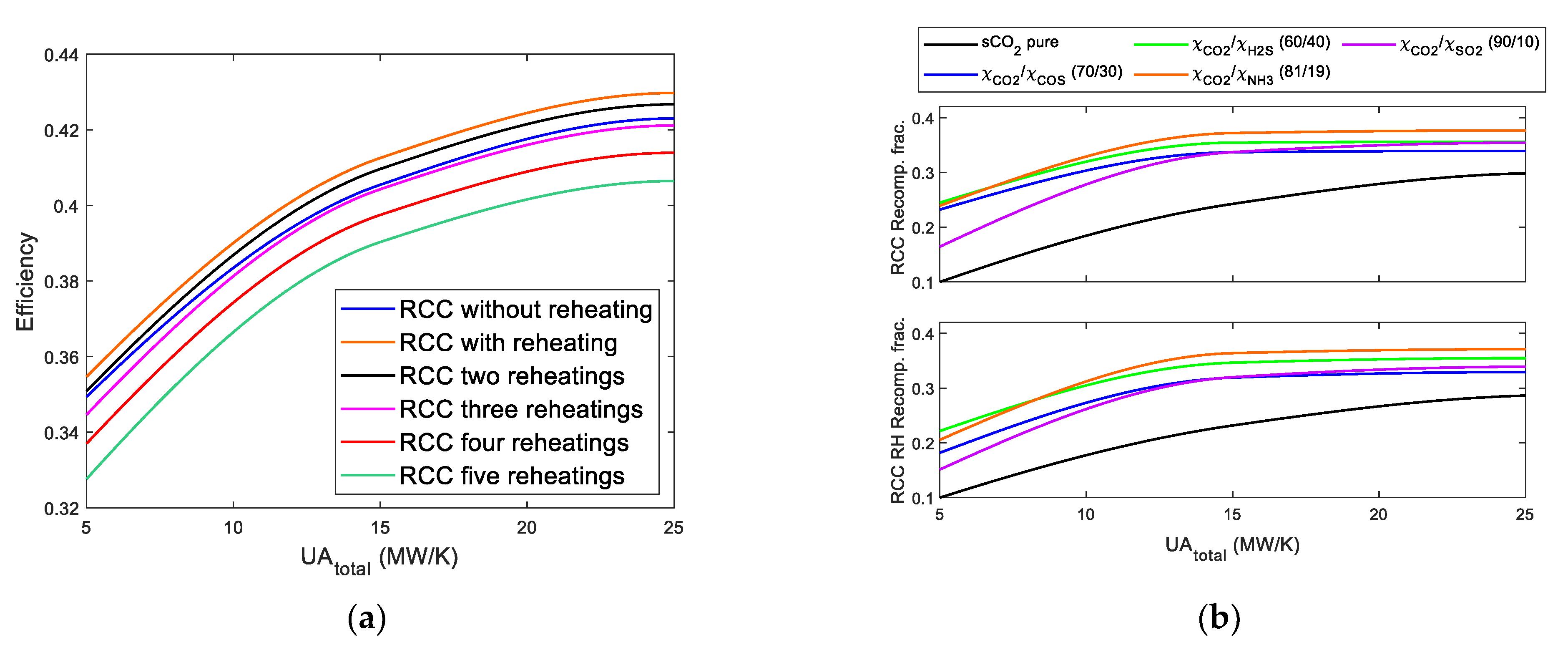
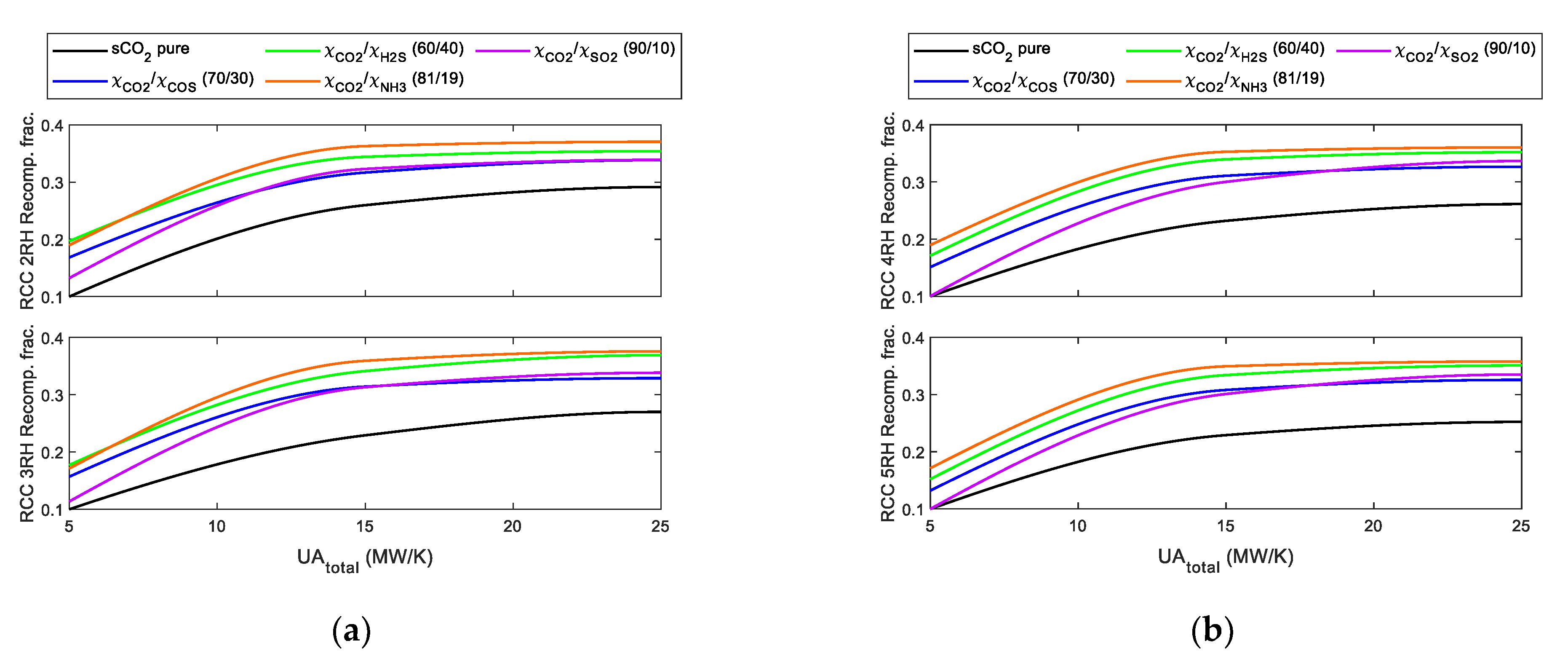
3.1. Impact of the Recompression Fraction on Recompression Brayton Cycles Using s-CO₂ Mixtures

When maximizing the recompression cycle’s efficiency, one of the essential parameters that must be analyzed is the recompression fraction, which is the fraction of fluid diverted to the recompressor. Research has shown that as the compressor inlet temperature decreases, the mass flow through the compressor increases [40]. However, in this study, the compressor inlet temperature is set at 51 °C so that each cycle configuration will have different optimized recompression fractions.

Studies [9,27] suggest that when the cycle operates with pure supercritical CO₂ as the working fluid, as the recuperator’s total conductance increases, the recompression fraction increases. This behavior also happens when the cycle uses mixtures based on supercritical CO₂ as a working fluid. As shown in Figure 13 and Figure 14, each mixture has different optimal recompression fractions for each recompression cycle configuration. As expected, when pure supercritical CO₂ and mixtures are used as the working fluid, as the recompression fraction increases, the cycle efficiency increases.

As shown in Figure 13b and Figure 14, the mixture composed of s-CO₂ and ammonia (81/19) needs to divert more mass flow to the recompressor to maximize its efficiency. However, it is not the one that gets the highest thermal efficiency. In contrast, the mixture composed of s-CO₂ and carbonyl sulfide (70/30) is the one that has the lowest mass flow rate the recompressor has to divert to maximize its efficiency, and it is the one that obtains the best thermal efficiency in the different configurations of the cycle.

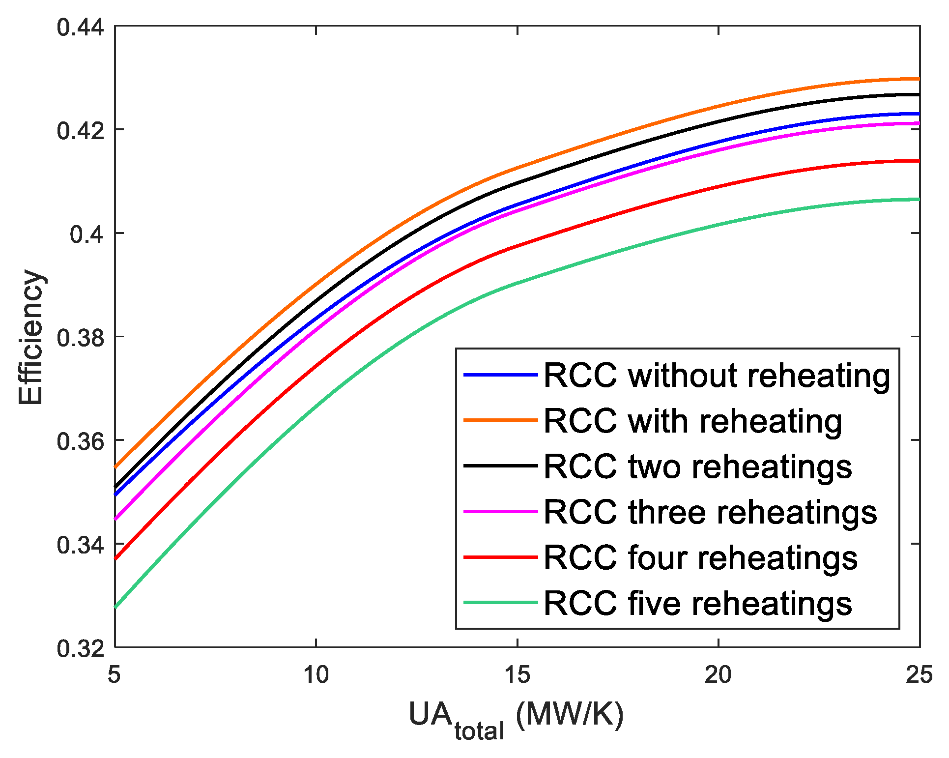
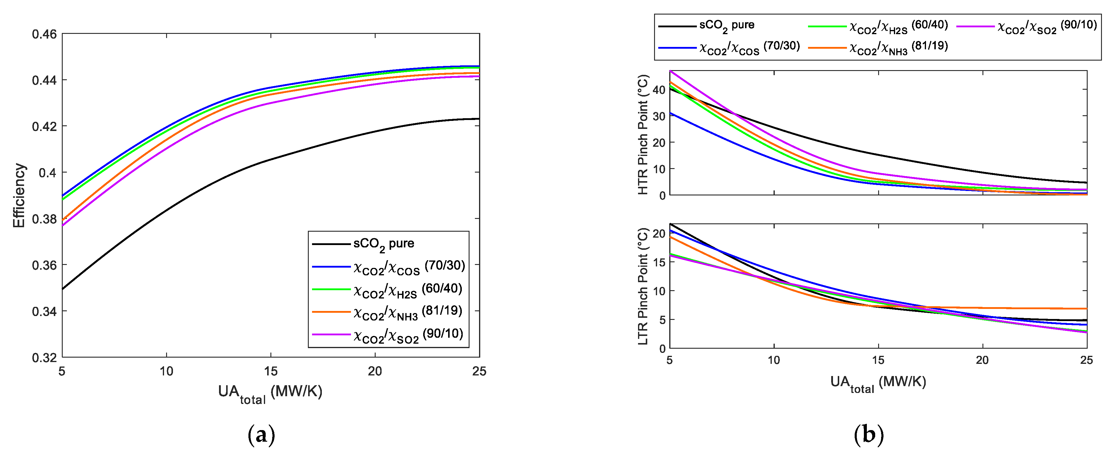
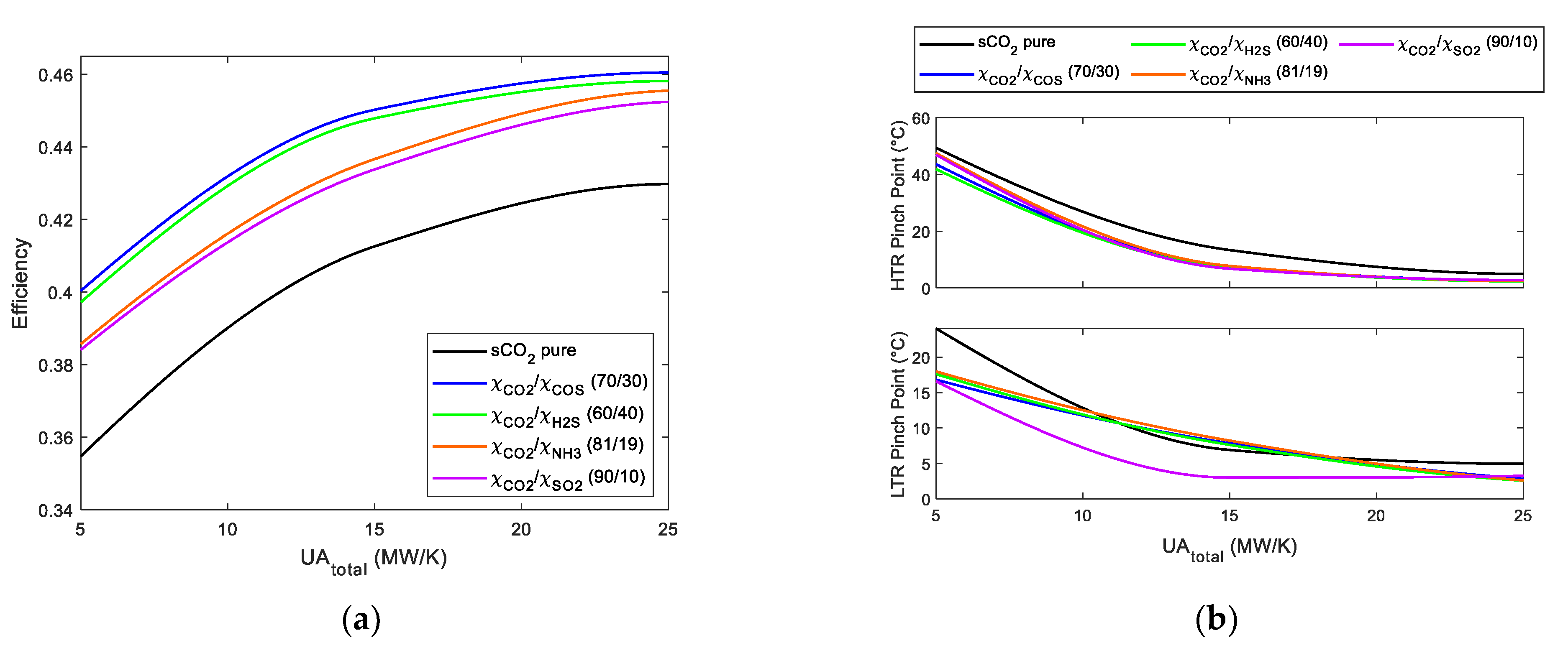
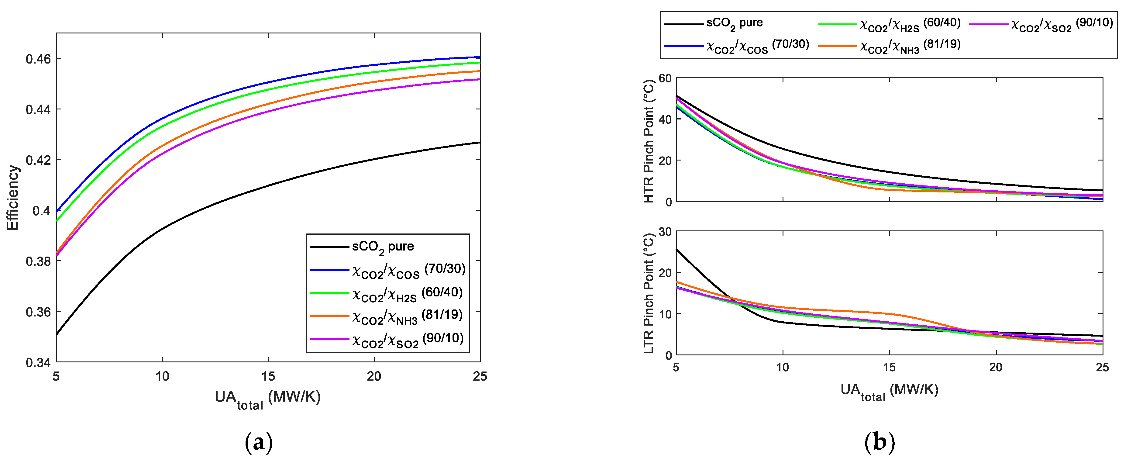
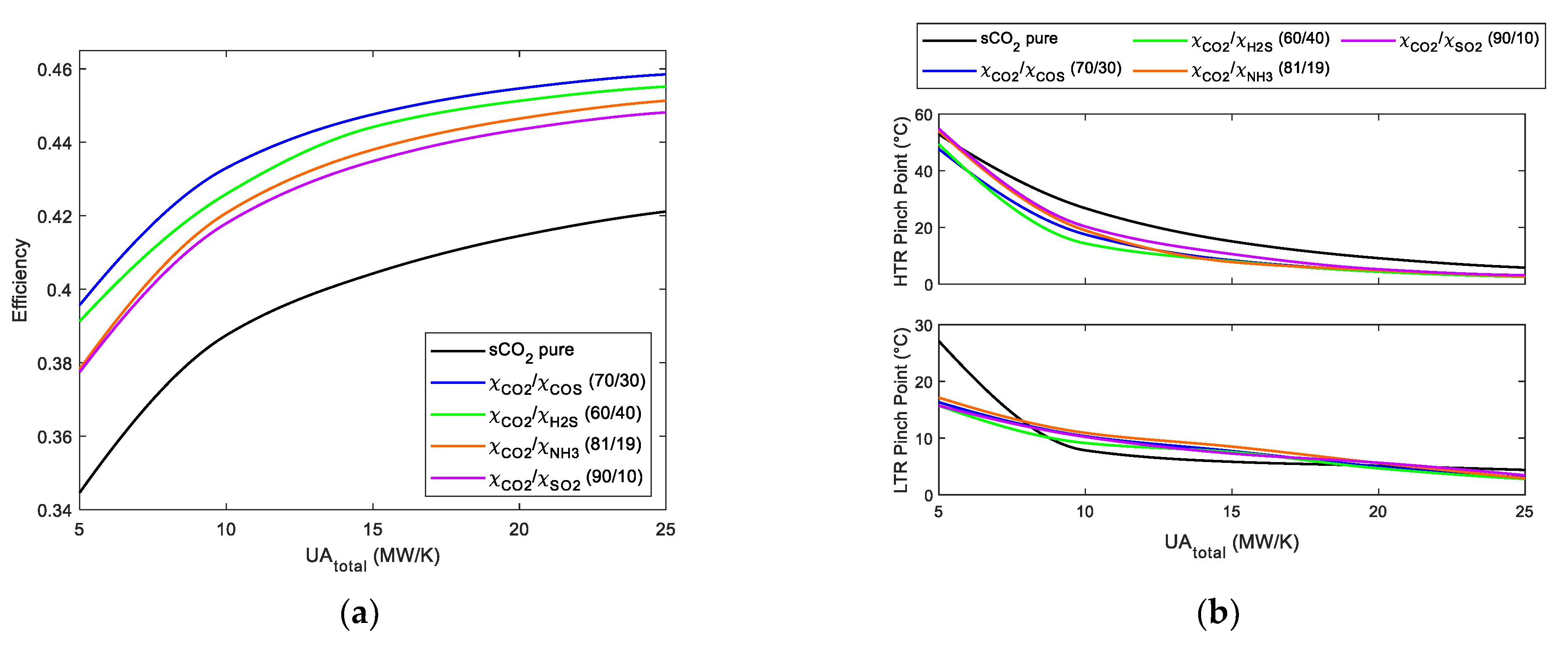
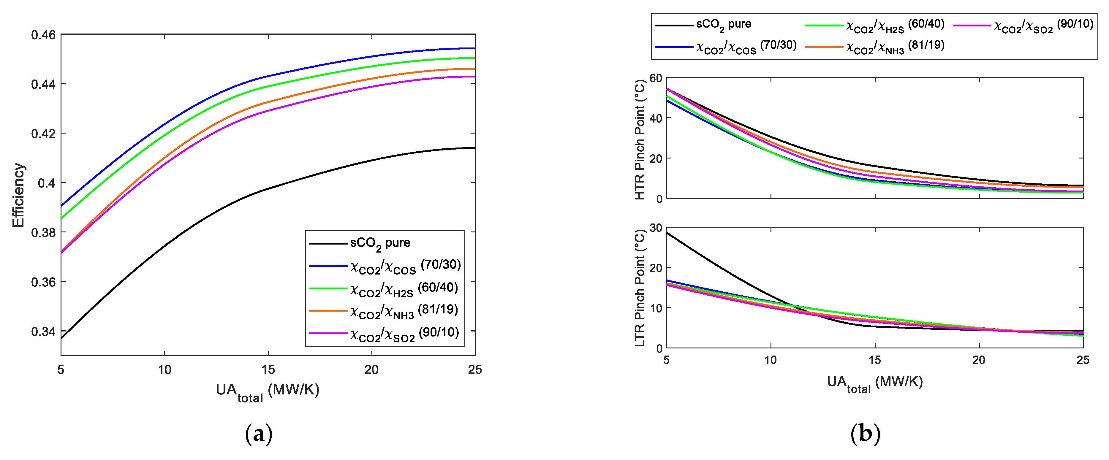
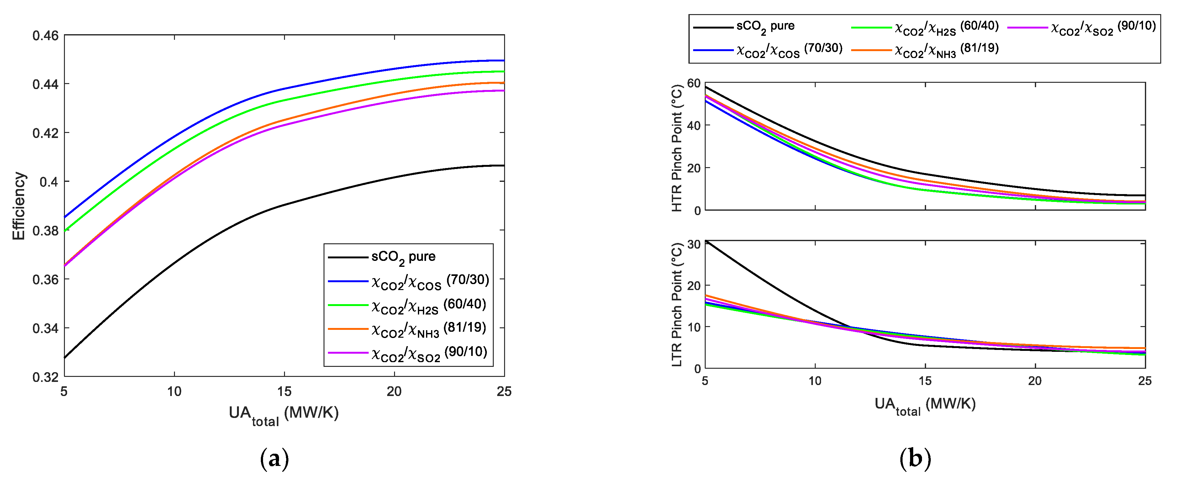
3.2. Impact on the Thermal Efficiency of Recompression Brayton Cycles Using s-CO₂ Mixtures

To explain the narrow difference in the four cases of supercritical CO₂ mixture’s performance, the cycle is divided into two separate cycles (see Figure 15).

The mass flow in CYCLE I is $\left(1-\gamma \right)\ast {\dot{m}}_{total}$ and through CYCLE II is $\gamma \ast {\dot{m}}_{total}$.

The efficiency of CYCLE II is very similar in all four mixtures within 7% of 0.3. The most efficient is the s-CO₂/NH₃, and the least efficient is the s-CO₂/COS. Interestingly, the s-CO₂/SO₂ mixture on cycle shows the second-best efficiency, 0.301, only 1.5% lower than the s-CO₂/NH₃.

The efficiency of CYCLE I is also quite similar in all four mixtures, being the maximum again the s-CO₂/NH₃ with 0.513 and the minimum the s-CO₂/SO₂ with 0.496, a 3.3% difference. The s-CO₂/COS mixture is the second poorest with 0.507, 1% lower than the s-CO₂/NH₃.

The better overall performance of the s-CO₂/COS, therefore, seems contradictory, but there is a relation between the recompression factor and efficiency:

$$\eta =\frac{W_{net}}{Q_{PHX}}=\frac{Q_{PH{X}_I}}{Q_{PHX}}\ast {\eta }_I+\frac{Q_{PH{X}_{II}}}{Q_{PHX}}\ast {\eta }_{II}=\left(1-\gamma \right)\ast {\eta }_I+\left(\gamma \right)\ast {\eta }_{II}$$

(22)

$$\frac{d\eta }{d\gamma }=-{\eta }_I+{\eta }_{II}=-0.2$$

(23)

It can be seen that if ${\eta }_I$ and ${\eta }_{II}$ were equal to 0.5 and 0.3 in all mixtures, the greater the recompression factor, the lower the efficiency would be. Indeed, this leads to ${\eta }_{COS}>{\eta }_{H_{2}S}>{\eta }_{N{H}_3}>{\eta }_{S{O}_2}$, following the general rule (see Figure 7, Figure 8, Figure 9, Figure 10, Figure 11 and Figure 12). However, the mixtures s-CO₂/COS and s-CO₂/SO₂ both have $\gamma =0.337$, and yet these two cases, in particular, show the greatest difference in overall efficiency. Given that the above formula still holds (Equations (22) and (23)), their proper ranking results from substituting their exact values for ${\eta }_I$ and ${\eta }_{II}$ are as expected. However, this behavior would require a physical explanation; there must exist a relation between the thermodynamic properties of the substances and the different values of recompression fraction.

The thermodynamic properties depend on the actual component being mixed with the supercritical CO₂ and the molar fraction. The $C_p$ is especially relevant to this topology. It can be observed that a poor heat exchange in LTR and HTR implies greater heat ($Q_{PHX}$) required to bring the fluid to turbine inlet conditions. It is therefore essential that $T_5$ ends as high as possible after the heat exchange at HTR, in other words: as near to $T_7$ as possible. For the same reason, that $T_9$ ends up as low as possible, as close to $T_2$ as possible. This will mean that the maximum amount of heat has been transferred from the hot flow (7–9) to the cold one (2–5). This depends on how close the temperature profiles of the hot and cold flows can be brought together in the heat exchange, which is determined by the heat capacities of the two flows.

If one flow has a much greater heat capacity than the other, a much greater amount of heat will need to be absorbed or released to have its temperature altered by one degree, so it will show a greater tendency to keep its temperature constant. Inevitably, this will keep the temperature drop between both flows apart, forcing large temperature differences at least at one of the ends of the heat exchanger, if not both. On the other hand, a design that could balance the heat capacities of both flows would allow to minimize the temperature drop. The purpose of $\gamma$ in the RCC topology is precisely to produce this effect, especially in the LTR heat exchange.

Let us analyze the LTR heat transfer process in more detail. The average specific heat of the cold (2–3) and hot flows (8–9) can be calculated:

$$\overline{c}p{,}_{2-3}=\frac{h_3-h_2}{T_3-T_2}$$

(24)

$$\overline{c}p{,}_{8-9}=\frac{h_8-h_9}{T_8-T_9}$$

(25)

A significant imbalance can be observed in

Table 3. Average specific heat of the cold (2–3) and hot flows (8–9).

	s-CO2/COS (70/30)	s-CO2/H2S (60/40)	s-CO2/NH3 (81/19)	s-CO2/SO2 (90/10)
$\overline{c}p{,}_{2-3}$ High Pressure (LTR)	1.74	2.07	2.28	1.85
$\overline{c}{p}_{,8-9}$ Low Pressure (LTR)	1.17	1.34	1.45	1.23

:

A lower mass flow on the cold side would compensate the heat capacities, and thus after deviating $\gamma$ away from the cold flow, it can be seen that both flows have been balanced, as outlined in

Table 4. Average specific heat of the cold flows balanced.

	s-CO2/COS (70/30)	s-CO2/H2S (60/40)	s-CO2/NH3 (81/19)	s-CO2/SO2 (90/10)
$\frac{{\overline{c}}_{p,high pressure}}{{\overline{c}}_{p,low pressure}} \left(LTR\right)$	1.49	1.54	1.58	1.50
$\frac{{\overline{C}}_{p,high pressure}}{{\overline{C}}_{p,low pressure}} \left(LTR\right)$	0.99	0.99	0.98	0.99

:

This ensures that the heat transfer is improved at the cost, however, of greater recompression and therefore having a greater share of the total power being produced by the least efficient cycle (Cycle II).

The main conclusion is that the best performance results from combining two phenomena; on one side, the actual efficiency of Cycles I and II, on the other, the specific heat imbalance between the low- and high-pressure isobars, which determines the need for recompression.

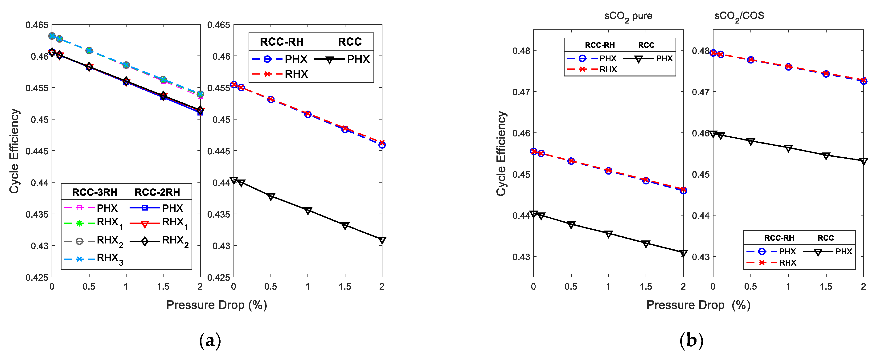
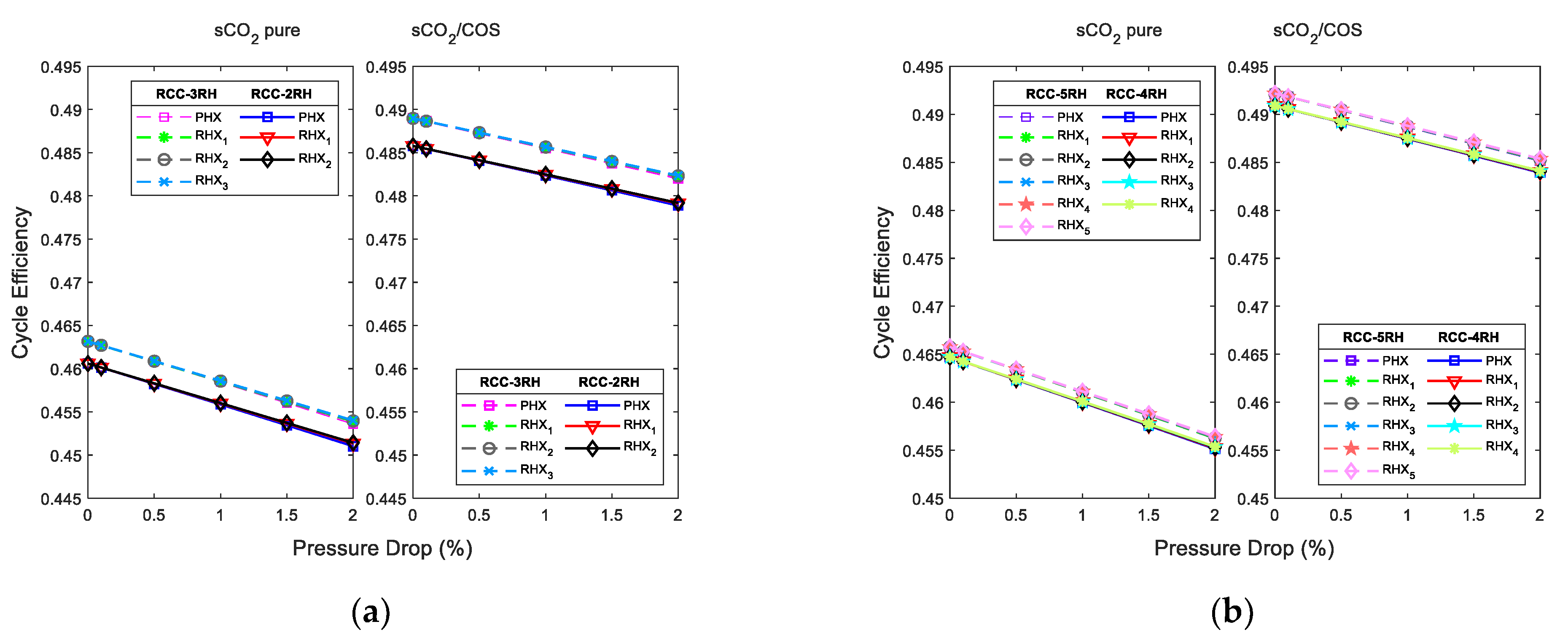
3.3. Impact of Pressure Drop on the Thermal Efficiency of the Brayton s-CO₂ Power Cycle

Figure 16 and Figure 17 show that the cycle’s efficiency decreases linearly when the pressure drop increases in the primary heat exchanger (PHX) and reheating heat exchanger (RHX). The pressure drop in the PHX has a greater impact on cycle efficiency than the pressure drops in the solar field RHX of the configurations studied when using pure s-CO₂ and s-CO₂ mixtures as working fluid. The lines overlap because the pressure drop has similar values.

3.4. Modeling of a PCHE

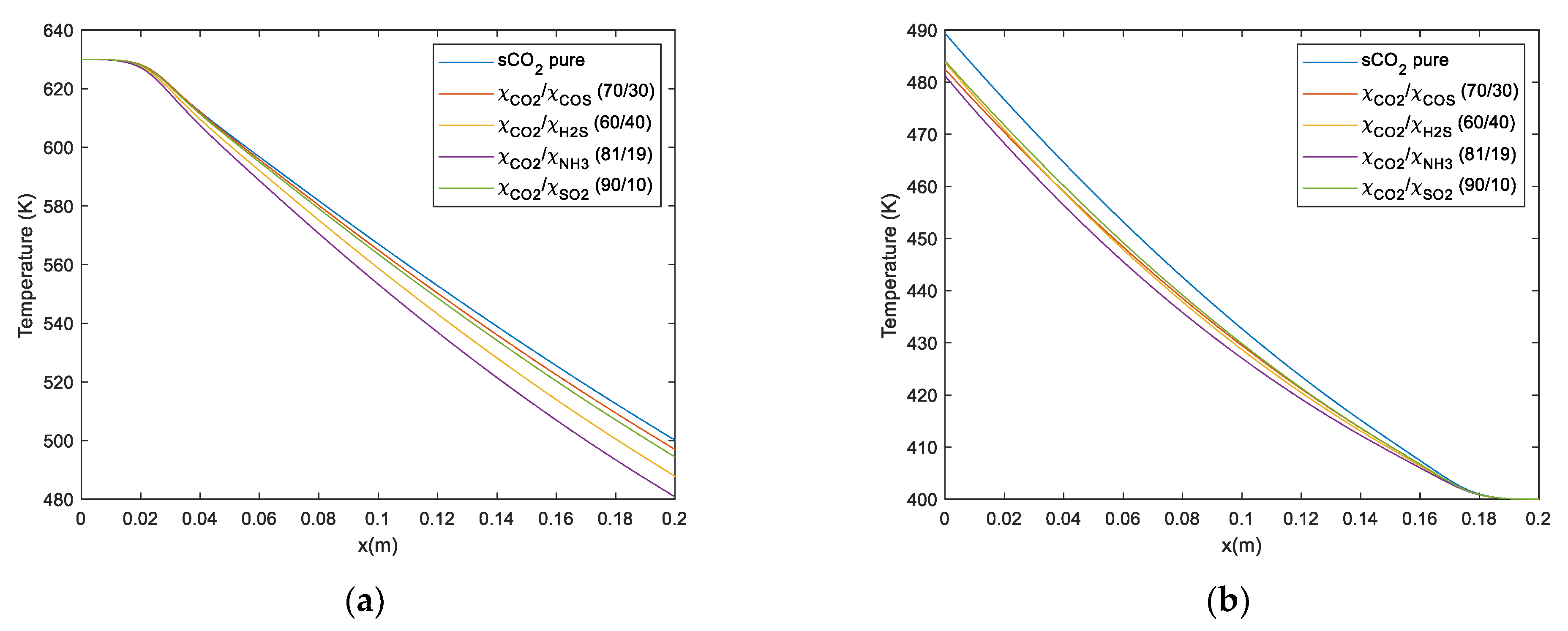
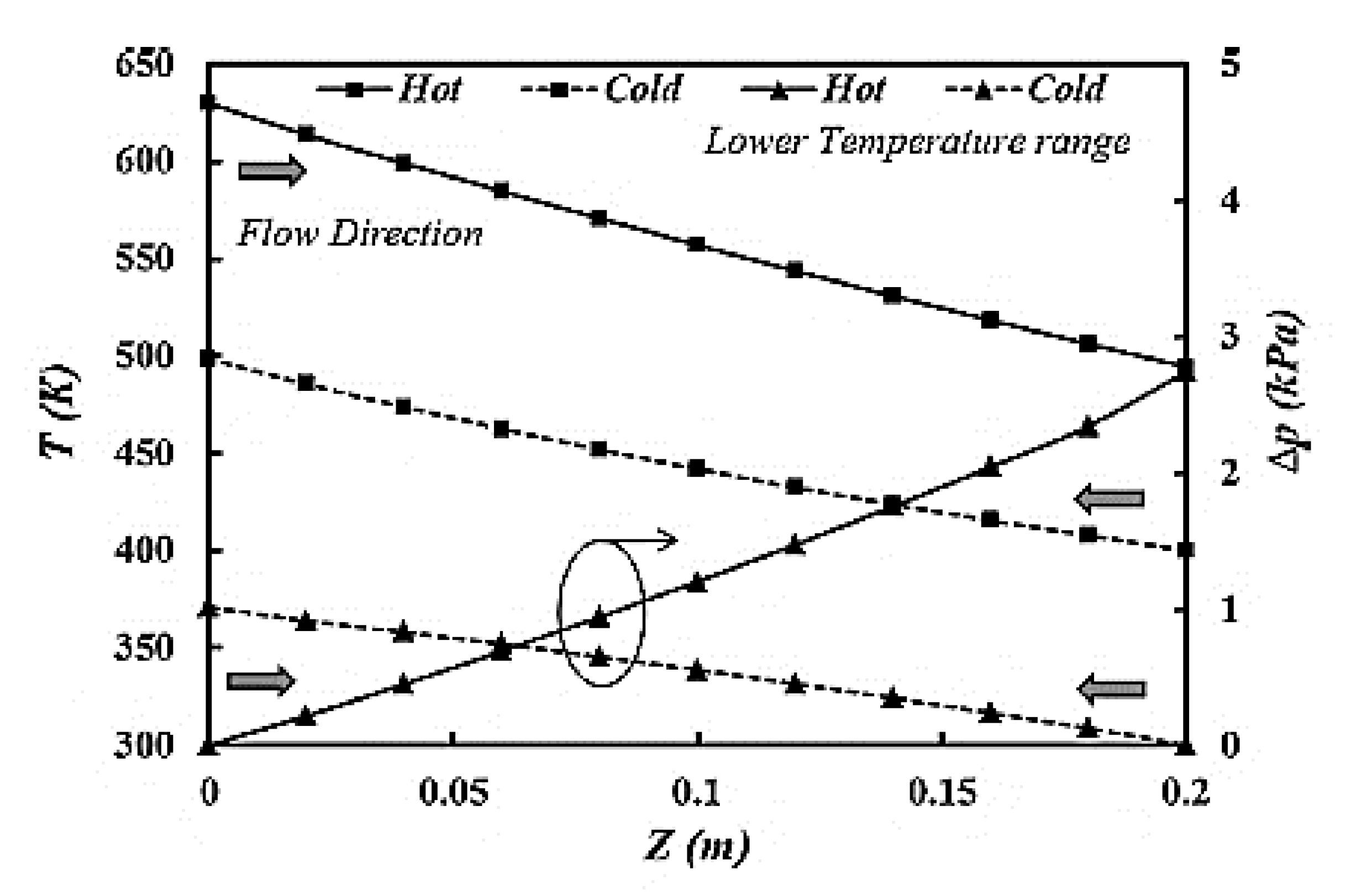
Regarding the PCHE,

Table 5. Boundary conditions.

Boundary	Boundary Conditions
Flow inlet	Inlet velocity
Flow outlet	Outlet pressure
Upper wall	Periodic
Bottom wall	Periodic
Side walls	Adiabatic
Front walls	Adiabatic
Back walls	Adiabatic

shows the boundary conditions used in all the simulations. Since the simulation does not cover the entire exchanger and considers that the device has many more heat exchange channels, periodic conditions have been used on the upper and lower walls. The rest of the device has been assumed adiabatic in order to simplify the analysis.

Table 6. Boundary numerical values.

Property	Hot s-CO2	Cold s-CO2
Temperature (K)	630	400
Pressure (bar)	90	225
Velocity (m/s)	4.702	0.8424

shows the main boundary values of the s-CO₂ flows and mixtures used in the simulation. These conditions were collected from the Meshram et al. (2016) study and were reproduced in the present study:

3.4.1. Temperature

Figure 18 shows the hot fluid temperature profile and the cold fluid of the different s-CO₂ mixtures used. As can be seen, the s-CO₂/NH₃ mixture is the one that presents the most significant slope in the temperature profile of the hot fluid; therefore, it is the one that cools the most. However, the opposite occurs in the temperature profile of the cold fluid. The fluid with the biggest outflow temperature is pure s-CO₂. The rest of the mixtures have similar behaviors, having intermediate values between s-CO₂ and the mixture s-CO₂/NH₃.

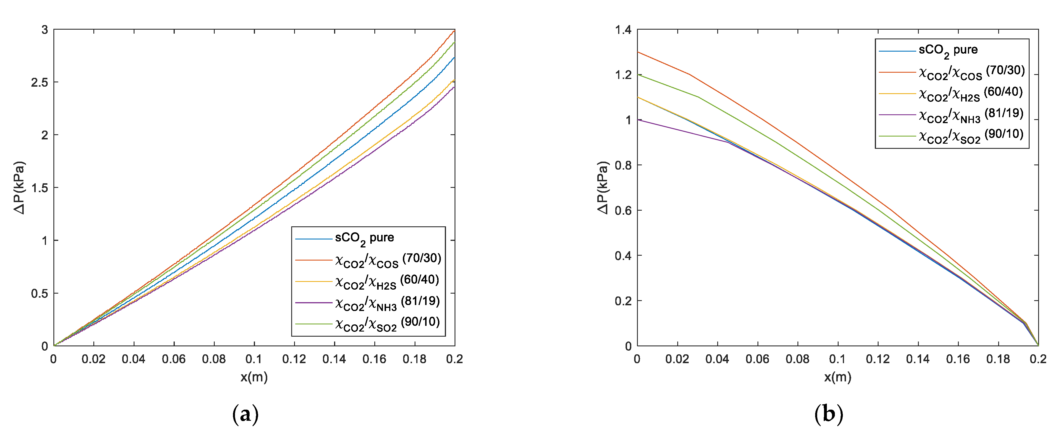
3.4.2. Pressure Loss

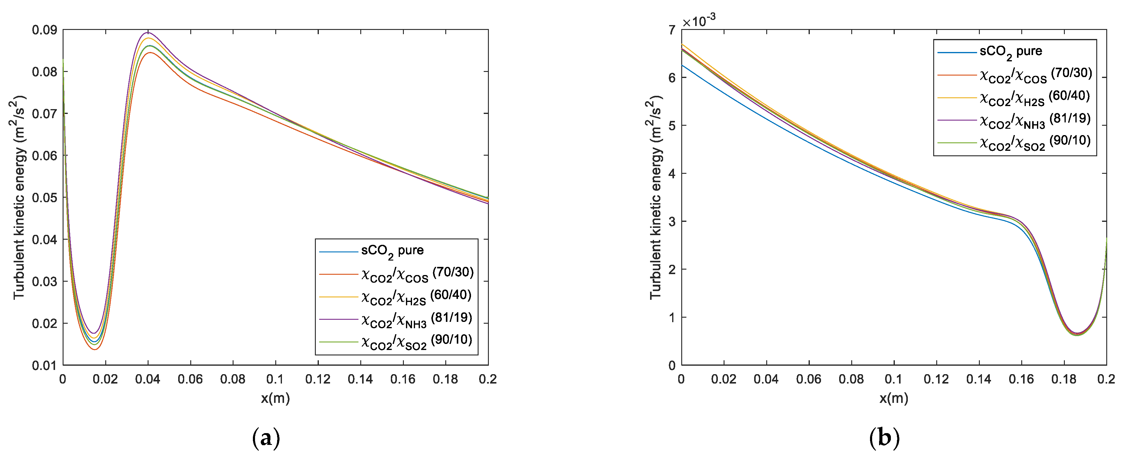
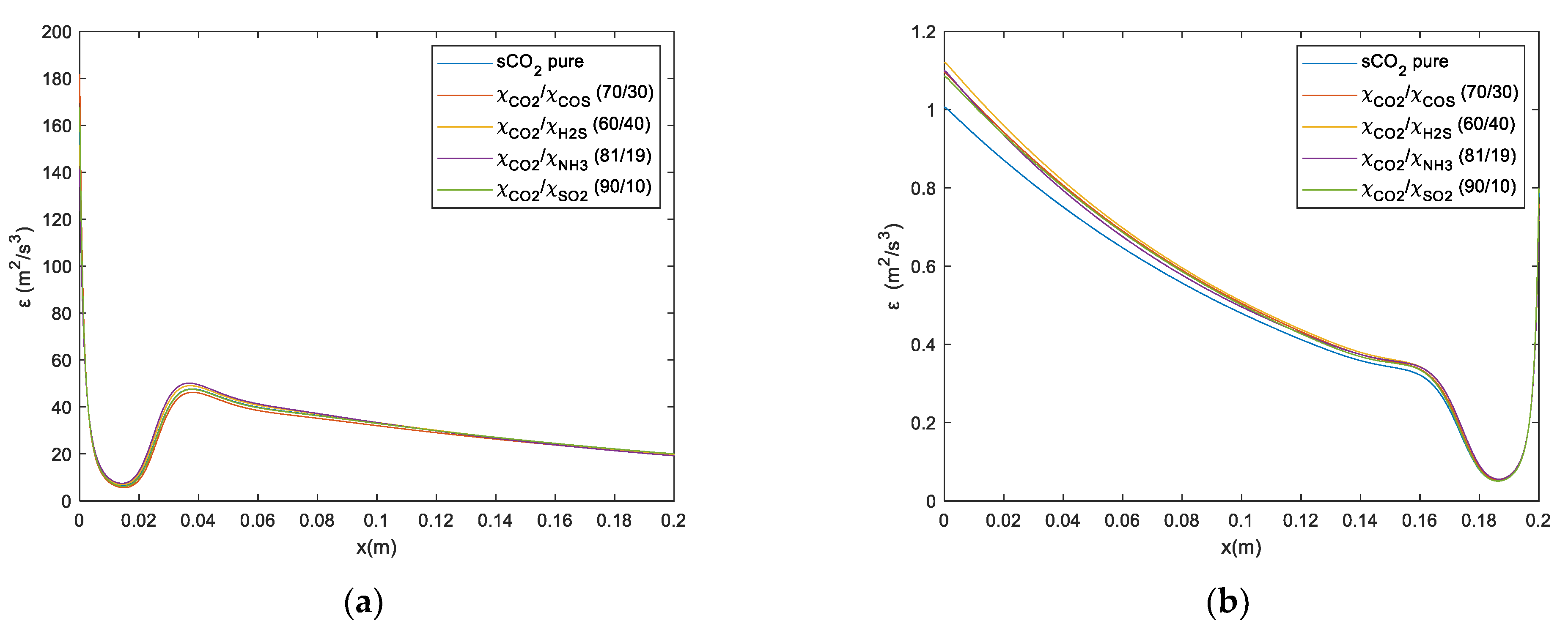
A parameter of great importance to study is the pressure drop in the exchanger channels. Figure 19 shows the pressure loss profile of the hot and cold fluid for the different s-CO₂ mixtures. It is observed that the hot fluid shows the greatest pressure loss, being even more than double the pressure drop of the cold fluid.

Under the different operating conditions, the s-CO₂/COS mixture shows the most significant pressure loss, albeit without reaching very high values, the maximum is 3.0 kPa. The s-CO₂/SO₂ mixture, albeit with lower values than the previous one, also shows a more significant pressure drop than pure s-CO₂. However, the mixtures s-CO₂/NH₃ and s-CO₂/H₂S show a minor pressure loss, the maximum being 2.45 kPa in the hot fluid and barely 1.0 kPa in the cold fluid for the mixture ammonia case.

3.4.3. Turbulence

A relevant parameter in heat exchange applications is turbulence since high turbulence encourages greater heat exchange in a fluid. Figure 20 shows the comparison of the turbulent kinetic energy $\left(k\right)$ of the different mixtures s-CO₂ throughout the control volume. As can be seen, the turbulent kinetic energy is very low in both the hot and cold conduits. However, the difference between the two flows is considerable; the hot flow’s turbulence is much higher than that of the cold flow. In this case, the turbulence is unstable at the inlet of the exchanger; however, it stabilizes and decreases from there upon reaching the 0.05 m point. This comportment is because the velocity profile enters the undeveloped domain.

The duct’s initial section is where the velocity profile develops, being homogeneous in the rest of the exchanger. As a result, the mixtures s-CO₂/NH₃ and s-CO₂/H₂S show higher values than the rest, although this difference is not significant.

Another important parameter related to turbulence in the $k-\epsilon$ model used is the dissipation of turbulent kinetic energy $\left(\epsilon \right)$. Figure 21 shows this dissipation ratio along with the profile of both hot and cold ducts. This parameter behaves similarly to that studied previously so that the dissipation rate of turbulent kinetic energy in hot fluid is again much higher than in cold fluid. Furthermore, all the mixtures show very similar behavior: the s-CO₂/NH₃ and s-CO₂/H₂S mixtures offer a slightly higher curve.

3.4.4. Surface Heat Flux and Exchange Area

Using the CFD software post-processor, the total surface heat exchanged flux was obtained as a fundamental parameter for this analysis, shown in

Table 7. Surface heat flux of each mixture.

	Surface Heat Flux (kW/m2)
s-CO2 pure	90.037
s-CO2/COS (70/30)	103.66
s-CO2/H2S (60/40)	91.25
s-CO2/NH3 (81/19)	92.32
s-CO2/SO2 (90/10)	98.64

. This parameter describes the total heat exchanged through the channel surfaces.

All the mixtures analyzed have a higher surface heat flux than pure s-CO₂. The mix with the most increased heat flow is s-CO₂/COS, followed by the mixture s-CO₂/SO₂. On the other hand, the mixtures s-CO₂/H₂S and s-CO₂/NH₃ show lower values, despite having higher heat flux than pure s-CO₂.

The average heat transfer coefficients and the Nusselt numbers shown in Table 6 were obtained using Equations (26) and (27):

$$\overline{h}=\frac{q}{T_B-T_W}$$

(26)

$$Nu=\frac{h{D}_h}{k}$$

(27)

where $T_B$ (K) is the average apparent temperature of the fluid (bulk temperature), $T_W$ (K), the average wall temperature, and $D_h$ (m) refers to the hydraulic diameter.

As might be expected, the mixtures that previously showed higher heat fluxes are those with higher heat transfer coefficients, reaching the s-CO₂/COS mix a coefficient of $1857.85 \mathrm{W}/{\mathrm{m}}^2\mathrm{K}$ for the hot flux (see

Table 8. Average surface heat transfer coefficient, Reynolds number, and Nusselt number of the different mixtures.

	Reynolds (Hot)	Reynolds (Cold)	Nusselt (Hot)	Nusselt (Cold)	$$\begin{gathered} {\overline{\mathit{h}}}_{\mathit{h}\mathit{o}\mathit{t}} \\ \left(\mathbf{W}/{\mathbf{m}}^2\mathbf{K}\right) \end{gathered}$$	$$\begin{gathered} {\overline{\mathit{h}}}_{\mathit{c}\mathit{o}\mathit{l}\mathit{d}} \\ \left(\mathbf{W}/{\mathbf{m}}^2\mathbf{K}\right) \end{gathered}$$
s-CO2 pure	23,833.96	21,080.52	43.986	43.706	1660.921	1851.094
s-CO2/COS (70/30)	27,341.45	20,772.70	51.536	47.386	1857.850	2149.123
s-CO2/H2S (60/40)	22,764.62	20,279.72	43.216	42.870	1685.415	2038.296
s-CO2/NH3 (81/19)	21,230.44	20,045.90	40.276	40.957	1698.906	2236.681
s-CO2/SO2 (90/10)	25,091.09	21,555.17	48.153	46.520	1786.100	2107.749

). However, in the cold flow, the s-CO₂/NH₃ mixture presents the highest heat transfer coefficient. Again, pure s-CO₂ shows a lower mean heat exchange coefficient in both hot and cold fluid.

In order to analyze the efficiency of the different mixtures, the necessary area of the heat exchanger must be taken into account to dissipate a fixed amount of heat of 8.9 MW, according to the reference study. Table 6 shows the main boundary values of the s-CO₂ flows and mixtures used in the simulation. These conditions have been collected from the Meshram et al. (2016). The area needed in the countercurrent supercritical recuperator to dissipate this amount of heat is obtained with Equation (28).

$$Q=UA∆T_{lm}$$

(28)

where $∆T_{lm}$ (K) is the mean logarithmic temperature difference, and $U$ (W/m²K) refers to the global heat transfer coefficient.

Table 9. Relevant parameters of each mixture.

	$$\begin{gathered} \mathbf{∆}{\mathit{T}}_{\mathit{l}\mathit{m}} \\ \left(\mathbf{K}\right) \end{gathered}$$	$$\begin{gathered} \overline{\mathit{U}} \\ \left(\mathbf{W}/{\mathbf{m}}^2\mathbf{K}\right) \end{gathered}$$	$$\begin{gathered} \mathbf{Area} \\ ({\mathbf{m}}^2) \end{gathered}$$
s-CO2 pure	119.443	854.067	14.704
s-CO2/COS (70/30)	120.491	968.866	12.849
s-CO2/H2S (60/40)	114.586	898.874	14.563
s-CO2/NH3 (81/19)	111.368	939.606	14.335
s-CO2/SO2 (90/10)	118.315	940.831	13.475

presents the most relevant parameters of the analysis to compare the efficiency of the different mixtures. As can be seen, all the mixtures offer better heat transfer performances than pure s-CO₂, being the s-CO₂/COS mixture, the one that presents a higher value of the global heat exchange coefficient. This behavior is reflected in the area of heat exchange necessary to dissipate the same amount of energy. In the s-CO₂/COS mixture, an area of 12.849 m² is required, representing a 12.62% reduction compared to the area needed to dissipate the same amount using pure s-CO₂. The mixture that shows the minor difference concerning pure s-CO₂ is the s-CO₂/H₂S mixture since it only reduces the necessary exchange area by 0.96%.

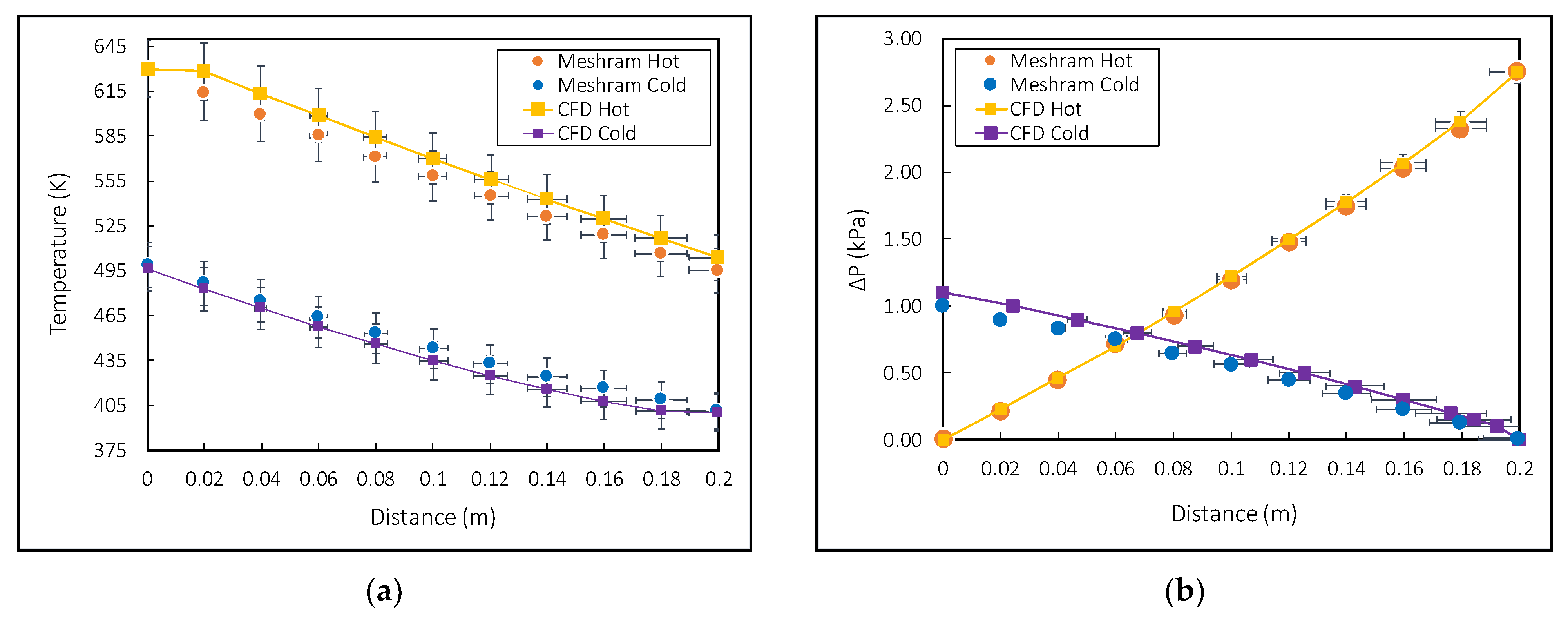
3.4.5. Model Validation

Figure 22 shows the results of the real gas model using the NITS model for the variables studied [31]. However, validation is limited to analyzing both the temperature profile and the pressure drop of the straight exchanger channel for the lowest temperature range (400 K for s-CO₂ cold and 630 K for s-CO₂ hot).

In Figure 23, comparing the temperature profile and the pressure drop obtained in the simulation with the reference study results are shown. As can be seen, the values obtained in the temperature profile simulation are very close to the reference values, the largest deviation being 2.35% in hot fluid and 2% in cold fluid. Moreover, in the case of pressure drop, the values obtained in the simulation are close to the reference values. Although the cold flow error seems high (maximum 16.3%), this is due to the low resolution of the simulation data. This comportment is due to the high orders of magnitude of the pressure (22.5 MPa). However, for the hot flow, as the pressure is lower (9 MPa), more accurate results have been obtained, so the error, in this case, is closer to reality; the maximum error is 6.7%.

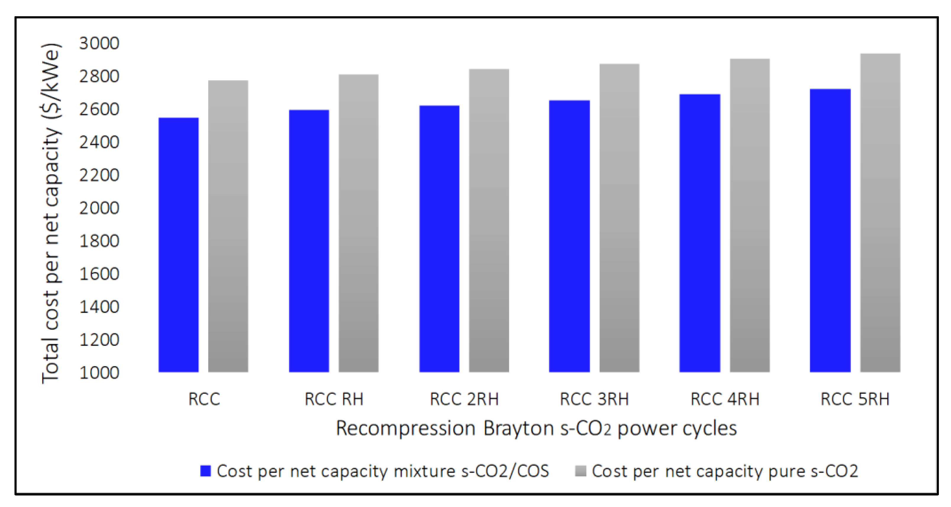
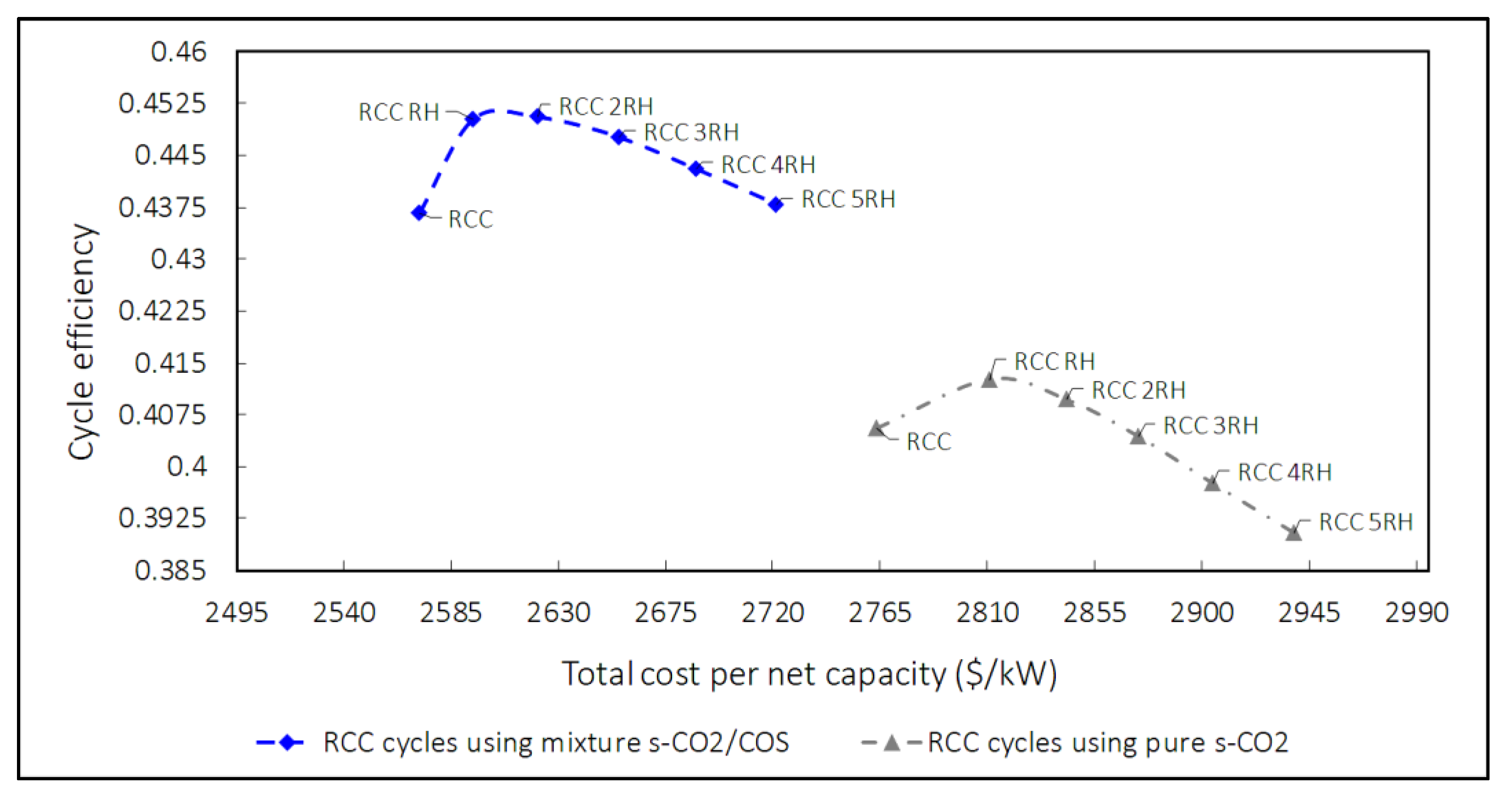
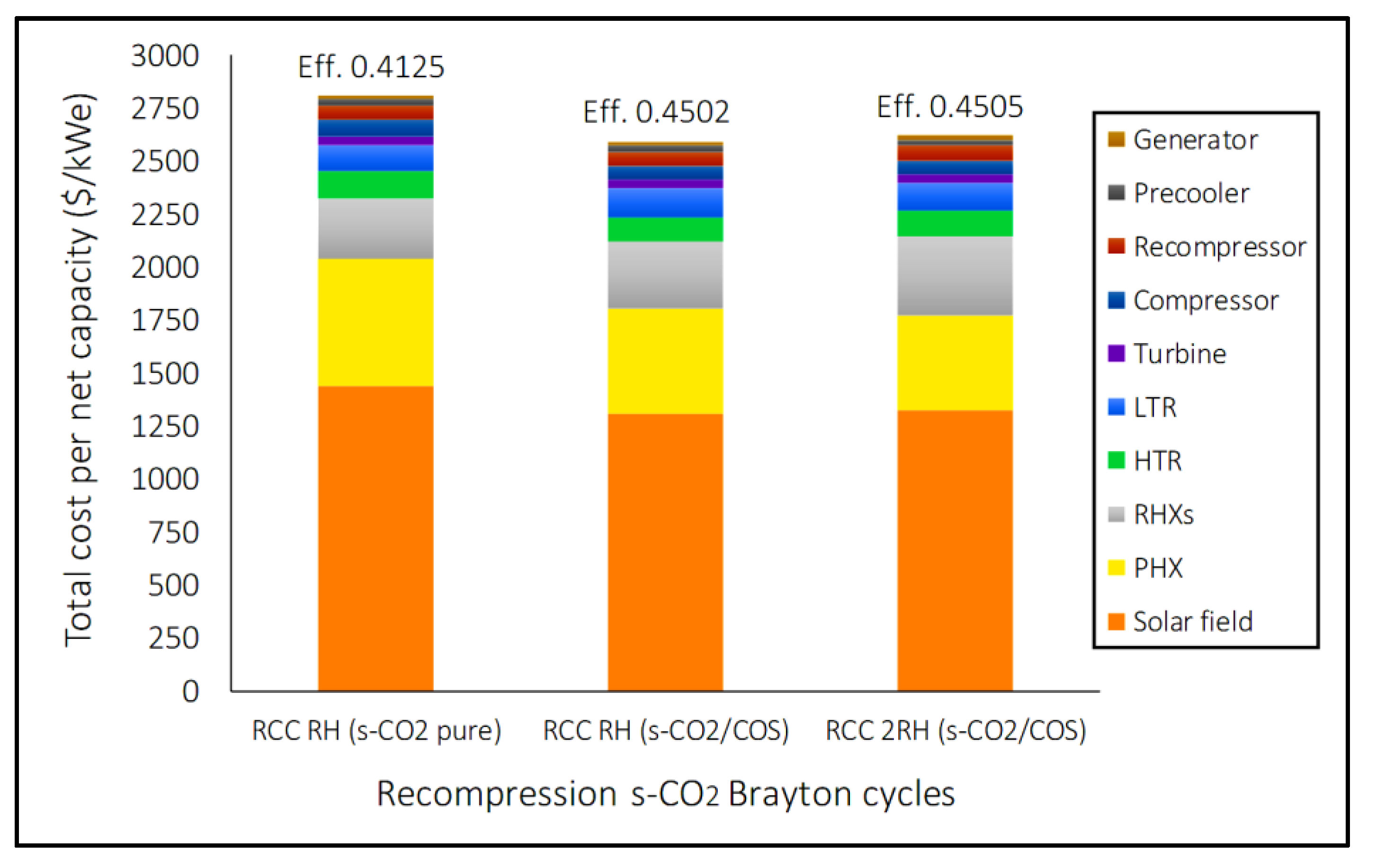
3.5. Cost Analysis of the Recompression Brayton s-CO₂ Power Cycles

After analyzing the impact of mixtures on cycle thermal efficiency, the various proposed configurations have also been investigated from an economic perspective. The cost models were taken from the literature for each major component used in the different recompression Brayton s-CO₂ power cycle configurations and fitted to the available limited data and cost estimates.

The cost correlations for each power block component (turbine, compressors, recuperators, etc.) are taken from [41]. In this research, the final cost of each component is determined with Equation (29), where $C$ is the cost of the component (expressed in $ USD), a and b are particular coefficients for each component, $SP$ is a scale parameter, and $f_T$ is the factor of temperature correction.

$$C=a\ast S{P}^b\ast f_T$$

(29)

The component costs of Brayton s-CO₂ power cycles can vary considerably depending on their operating temperature. The temperature correction factor, Equation (25), includes cost correction factors considering a selection of materials and thickness based on operating pressure and temperature. Where $T_{bp}$ is the temperature of the inflection point, which is set at 550 °C, and marks the temperature from which its increase makes it necessary to use other specific materials for a higher range of temperatures.

$$f_T=\left\{\begin{array}{cc}1& if T_{máx}<T_{bp}\\ 1+c\ast \left(T_{máx}-T_{bp}\right)+d\ast {\left(T_{máx}-T_{bp}\right)}^2& if T_{máx}\ge T_{bp}\end{array}\right\}$$

(30)

The coefficients a, b, c, and d shown in Equations (29) and (30) are shown in

Table 10. Scale parameters and coefficients for the correlations Equations (29) and (30) of the components.

Components	Scaling Parameters	Coefficients
		a	b	c	d
Axial Turbine	Wsh (MWth)	182,600	0.5561	0	1.11 × 10−4
IG centrifugal compressors	Wsh (MWth)	1,230,000	0.3992	0	0
Generators	We (MWe)	108,900	0.5463	0	0
Recuperators	UA (W/K)	49.45	0.7544	0.02141	0
Cooler	UA (W/K)	32.88	0.75	0	0

for each component, together with the scale parameters, $SP$.

For the cost’s calculation of the primary heat exchanger, the reference is used [9], where the cost of the PHX is calculated using Equation (31), this is a function of conductance, $U{A}_{PHX}$ [kW/K].

$$C_{PHX}=3500\ast U{A}_{PHX}$$

(31)

The same correlations adopted in the NREL System Advisor Model (SAM 2020.11.29) [42] have been used for the solar field costs with parabolic trough technology. A constant cost is assumed based on the thermal power required in the PHX and RHXs, for this case, for a temperature of 550 °C of the HTF the value is 590 $/kW_th that includes: solar field with PTC, site improvement, land, HTF system, contingency; and engineering, procurement, and construction (EPC) costs.

Figure 24 compares total costs per net capacity using pure supercritical CO₂ and the binary mixture of carbon dioxide and carbonyl sulfide in the supercritical state (a mixture that provides the best efficiency with mole fraction (70/30) as working fluids in the cycle. The results show that the cost of the simple recompression cycle with pure supercritical CO₂ as the working fluid is around 6.92% more expensive than when using the CO₂/COS (70/30) mixture. However, when the recompression cycle has the most complex configuration, the cycle’s cost when using pure supercritical CO₂ becomes more expensive by about 7.41% than when using the CO₂/COS mixture. This behavior occurs because if the mixture is used in that mole fraction, its density is greater than that of pure supercritical CO₂, which reduces the conductance values (UA). Therefore, the size of the components is reduced.

Figure 25 shows the optimal efficiencies for each recompression cycle configuration compared to the total cost per net capacity for a UA 15,000 kW/K. The results show, as previously concluded, that the binary CO₂/COS mixture with mole fraction (70/30), respectively, has a positive impact increasing the cycle efficiency compared to pure supercritical CO₂. However, as the cycle configuration becomes more complex, the efficiency decreases; this is because the pressure drops in the new components negatively influence the efficiency.

Therefore, the optimal configuration using pure supercritical CO₂ as the working fluid is RCC-RH with efficiency values of 41.25% and a total cost of around 2811.23 $/kWe, in contrast, when using the binary CO₂/COS mixture as a working fluid. The configurations that present the best values in terms of efficiency and cost are the RCC-RH with values of 45.02% and 2594.45 $/kWe; and RCC-2RH with values of 45.05% and 2621.23 $/kWe, respectively.

Figure 26 show a comparison of total costs per net capacity as the sum of the components costs and the solar field when using pure supercritical CO₂ and the binary mixture of carbon dioxide and carbonyl sulfide in a supercritical state (a mixture provides the best efficiency with mole fraction (70/30) as working fluids in the cycle). The solar field costs are the most representative in all cases, followed by the primary heat exchanger costs and reheat heat exchangers. As mentioned above, the LTR and HTR recuperators’ conductance were optimized to maximize efficiency, and the summation has fixed values between 5000 and 25,000 kW/K. In this sense, the cost analysis was carried out for a recuperators’ total conductance (UA) of 15,000 kW/K.

4. Conclusions

One of this study’s main objectives was to evaluate the impact of mixtures that increase the critical temperature on thermal efficiency when used in recompression Brayton s-CO₂ power cycles as a working fluid. The results showed that such mixtures have a positive impact already that increases efficiency; in this way, the mixture with the best efficiency in all configurations is made up of carbonyl sulfide followed by the mixtures with hydrogen sulfide, ammonia, and sulfur dioxide.

The best performance of mixtures on Brayton s-CO₂ power cycles results from the combination of two phenomena; on one side, the actual efficiency of Cycles I and II analyzed in Section 3.2; on the other, the specific heat imbalance between the low- and high-pressure isobars, which determines the need for recompression.

The heat capacities on the cold side balance out after diverting more mass flow to the recompressor. Therefore, the higher the mass flow rate diverted to the recompressor, the better the heat capacity imbalance in the heat exchanged in LTR will be compensated for. However, efficiency is penalized because more work is produced in the less efficient cycle. Therefore, the s-CO₂/COS mixture, by diverting less mass flow to the recompressor, has less power in the less efficient cycle and more power in the more efficient cycle.

Additionally, it was considered to carry out the analysis by adding pressure drops in the components of the recompression Brayton s-CO₂ cycle. The results showed that as the configuration of the cycle becomes more complex, there is a more significant penalty in the efficiency. The component that produces the most significant negative impact is the primary heat exchanger. However, blends still achieve higher efficiency compared to pure supercritical CO₂. In configurations of up to three reheatings, it is observed that depending on the mixture used, thermal efficiency increases between two and four points concerning pure s-CO₂. Whereas, in configurations with four and five reheatings, it can increase between three and six points.

Another objective that must be highlighted is the validation of the model for PCHE that uses supercritical CO₂ pure as heat transfer fluid, and the comparative study with the different mixtures has been successfully carried out. It is concluded that the increase in performance in the Brayton cycle of certain mixtures that raise the temperature of the critical point is directly correlated with the increase in the performance of a PCHE recuperator. All the mixtures studied have shown better global heat transfer coefficients than pure supercritical carbon dioxide, which represents a reduction for the mixtures s-CO₂/COS (70/30), s-${\mathrm{CO}}_2/{\mathrm{H}}_2\mathrm{S}$ (60/40), s-${\mathrm{CO}}_2/{\mathrm{NH}}_3$ (81/19) and s-${\mathrm{CO}}_2/{\mathrm{SO}}_2$ (90/10) of 12.62%, 0.96%, 2.51%, and 8.36%, respectively in the total heat exchange area.

This inference can be extrapolated directly into considerable economic savings for high power ranges. Furthermore, these results yield highly relevant conclusions since they confirm the possibility of continuing Brayton cycles’ improvement using PCHE exchangers as regenerators. It is, therefore, a step forward in the investigation of supercritical Brayton cycles, which in the future may represent essential advances in the mitigation of greenhouse gas emissions.

On the other hand, an additional analysis for different PCHE geometries would yield parallel research lines of particular interest. For example, modifications in the diameter of the channels or comparisons between straight channels and zigzag channels, such as those made in the study by Meshram et al. (2016) for pure s-CO₂, would provide additional information on the behavior of the different supercritical mixtures with the temperature profile and the pressure drop under these geometries.

Finally, a techno-economic analysis was carried out, the results of which show that the more complex configurations incur high costs. Due to the pressure drop, they obtain lower efficiency. In this way, when we use supercritical CO₂ pure as the working fluid, the configuration recompression with reheating gains greater efficiency with a value of 41.25% and, in turn, has the lowest cost of 2811 $/kWe. Whereas, if the cycle uses the mixture composed of carbonyl sulfide, the configuration recompression with two reheating gains greater efficiency with a value the 45.05% and has a cost of 2621 $/kWe. However, in mixing, the configuration that obtains the lowest cost is the single reheating (RCC-RH), which also has high efficiency. Their values are 2594.5 $/kWe and 45.02%. Therefore, using the mixture costs 7.70% less than using the standard fluid (s-CO₂) in the same configuration (RCC RH).

There are several required future works related to the presented results, not only related to a more in-depth analysis in terms of CFD and s-CO₂ mixtures from the energetic point of view, but also in terms of chemical compatibility of mixtures and materials, among others.

References

1. Trevisan, S.; Guédez, R.; Laumert, B. Thermo-economic optimization of an air driven supercritical CO2 Brayton power cycle for concentrating solar power plant with packed bed thermal energy storage. Sol. Energy 2020, 211, 1373–1391. [Google Scholar] [CrossRef]
2. IRENA. Renewable Capacity Statistics 2020, Internacional Renovable Energía Agencia; International Renewable Energy Agency (IRENA): Abu Dhabi, United Arab Emirates, 2020. [Google Scholar]
3. Yin, J.M.; Zheng, Q.Y.; Peng, Z.R.; Zhang, X.R. Review of supercritical CO2 power cycles integrated with CSP. Int. J. Energy Res. 2020, 44, 1337–1369. [Google Scholar] [CrossRef]
4. Siddiqui, M.E.; Almitani, K.H. Proposal and Thermodynamic Assessment of S-CO2 Brayton Cycle Layout for Improved Heat Recovery. Entropy 2020, 22, 305. [Google Scholar] [CrossRef] [PubMed] [Green Version]
5. Crespi, F.; Gavagnin, G.; Sánchez, D.; Martínez, G.S. Supercritical carbon dioxide cycles for power generation: A review. Appl. Energy 2017, 195, 152–183. [Google Scholar] [CrossRef]
6. Turchi, C.S.; Ma, Z.; Neises, T.W.; Wagner, M.J. Thermodynamic study of advanced supercritical carbon dioxide power cycles for concentrating solar power systems. J. Sol. Energy Eng. 2013, 135. [Google Scholar] [CrossRef]
7. Al-Sulaiman, F.A.; Atif, M. Performance comparison of different supercritical carbon dioxide Brayton cycles integrated with a solar power tower. Energy 2015, 82, 61–71. [Google Scholar] [CrossRef]
8. Marchionni, M.; Bianchi, G.; Tassou, S.A. Techno-economic assessment of Joule-Brayton cycle architectures for heat to power conversion from high-grade heat sources using CO2 in the supercritical state. Energy 2018, 148, 1140–1152. [Google Scholar] [CrossRef]
9. Neises, T.; Turchi, C. Supercritical carbon dioxide power cycle design and configuration optimization to minimize levelized cost of energy of molten salt power towers operating at 650 °C. Sol. Energy 2019, 181, 27–36. [Google Scholar] [CrossRef]
10. Linares, J.I.; Montes, M.J.; Cantizano, A.; Sánchez, C. A novel supercritical CO2 recompression Brayton power cycle for power tower concentrating solar plants. Appl. Energy 2020, 263, 114644. [Google Scholar] [CrossRef]
11. Wang, K.; He, Y.L.; Zhu, H.H. Integration between supercritical CO2 Brayton cycles and molten salt solar power towers: A review and a comprehensive comparison of different cycle layouts. Appl. Energy 2017, 195, 819–836. [Google Scholar] [CrossRef]
12. Wang, K.; Li, M.J.; Guo, J.Q.; Li, P.; Liu, Z.B. A systematic comparison of different S-CO2 Brayton cycle layouts based on multi-objective optimization for applications in solar power tower plants. Appl. Energy 2018, 212, 109–121. [Google Scholar] [CrossRef]
13. Valencia-Chapi, R.; Coco-Enríquez, L.; Muñoz-Antón, J. Supercritical CO2 Mixtures for Advanced Brayton Power Cycles in Line-Focusing Solar Power Plants. Appl. Sci. 2020, 10, 55. [Google Scholar] [CrossRef] [Green Version]
14. Binotti, M.; Di Marcoberardino, G.; Iora, P.; Invernizzi, C.; Manzolini, G. Scarabeus: Supercritical carbon dioxide/alternative fluid blends for efficiency upgrade of solar power plants. AIP Conf. Proc. 2020, 2303. [Google Scholar] [CrossRef]
15. Yu, A.; Su, W.; Zhao, L.; Lin, X.; Zhou, N. New Knowledge on the Performance of Supercritical Brayton Cycle with CO2-Based Mixtures. Energies 2020, 13, 1741. [Google Scholar] [CrossRef] [Green Version]
16. Vesely, L.; Dostal, V.; Stepanek, J. Effect of gaseous admixtures on cycles with supercritical carbon dioxide. In Turbo Expo: Power for Land, Sea, and Air; American Society of Mechanical Engineers: New York, NY, USA, 2016. [Google Scholar]
17. Vesely, L.; Manikantachari, K.R.V.; Vasu, S.; Kapat, J.; Dostal, V.; Martin, S. Effect of impurities on compressor and cooler in supercritical CO2 cycles. J. Energy Resour. Technol. 2019, 141. [Google Scholar] [CrossRef]
18. Guo, J.Q.; Li, M.J.; Xu, J.L.; Yan, J.J.; Wang, K. Thermodynamic performance analysis of different supercritical Brayton cycles using CO2-based binary mixtures in the molten salt solar power tower systems. Energy 2019, 173, 785–798. [Google Scholar] [CrossRef]
19. Ma, Y.; Liu, M.; Yan, J.; Liu, J. Performance investigation of a novel closed Brayton cycle using supercritical CO2-based mixture as working fluid integrated with a LiBr absorption chiller. Appl. Therm. Eng. 2018, 141, 531–547. [Google Scholar] [CrossRef]
20. González-Portillo, L.F.; Muñoz-Antón, J.; Martínez-Val, J.M. Thermodynamic analysis of multi-heating cycles working around the critical point. Appl. Therm. Eng. 2020, 174, 115292. [Google Scholar] [CrossRef]
21. González-Portillo, L.F. Un Nuevo Concepto de Optimización de la Ingeniería Térmica: El Ciclo Pericrítico con Multicalentamiento y su Aplicación a la Energía Solar de Concentración. Ph.D. Thesis, ETSI Industriales (UPM), Madrid, Spain, 2019. [Google Scholar]
22. Ngo, T.L.; Kato, Y.; Nikitin, K.; Ishizuka, T. Heat transfer and pressure drop correlations of microchannel heat exchangers with S-shaped and zigzag fins for carbon dioxide cycles. Exp. Therm. Fluid Sci. 2007, 32, 560–570. [Google Scholar] [CrossRef]
23. Kar, S.P. CFD Analysis of Printed Circuit Heat Exchanger. Ph.D. Thesis, National Institute of Technology, Rourkela, India, 2007. Available online: http://ethesis.nitrkl.ac.in/4337/1/Cfd_Analysis_Of_Printed_Circuit_Heat.pdf (accessed on 16 February 2020).
24. Kim, S.G.; Lee, Y.; Ahn, Y.; Lee, J.I. CFD aided approach to design printed circuit heat exchangers for supercritical CO2 Brayton cycle applications. Ann. Nucl. Energy 2016, 92, 175–185. [Google Scholar] [CrossRef]
25. Jeong, W.S.; Lee, J.I.; Jeong, Y.H. Potential improvements of supercritical recompression CO2 Brayton cycle by mixing other gases for the power conversion system of an SFR. Nucl. Eng. Des. 2011, 241, 2128–2137. [Google Scholar] [CrossRef]
26. Coco-Enríquez, L. Nueva Generación de Centrales Termosolares con Colectores Solares Lineales Acoplados a Ciclos Supercríticos de Potencia. Ph.D. Thesis, ETSI Industriales (UPM), Madrid, Spain, 2019. [Google Scholar] [CrossRef]
27. Dyreby, J.J. Modeling the Supercritical Carbon Dioxide Brayton Cycle with Recompression. Ph.D. Thesis, University of Wisconsin-Madison, Madison, WI, USA, 2014. Available online: https://sel.me.wisc.edu/publications/theses/dyreby14.zip (accessed on 20 March 2020).
28. Thermoflow Inc. Thermoflow Software. 2021. Available online: http://www.thermoflow.com/ (accessed on 8 January 2020).
29. Lemmon, E.W.; Bell, I.H.; Huber, M.L.; McLinden, M.O. NIST Standard Reference Database 23: Reference Fluid Thermodynamic and Transport Properties-REFPROP; Version 10.0; National Institute of Standards and Technology: Gaithersbg, MD, USA, 2018. Available online: https://www.nist.gov/sites/default/files/documents/2018/05/23/refprop10a.pdf (accessed on 20 June 2020).
30. Kulhánek, M.; Dostál, V. Thermodynamic Analysis and Comparison of Supercritical Carbon Dioxide Cycles. 2011. Available online: http://www.sCO2powercyclesymposium.org/resource_center/system_concepts/thermodynamic-analysis-and-comparison-of-supercritical-carbon-dioxide-cycles (accessed on 13 October 2020).
31. Meshram, A.; Jaiswal, A.K.; Khivsara, S.D.; Ortega, J.D.; Ho, C.; Bapat, R.; Dutta, P. Modeling and analysis of a printed circuit heat exchanger for supercritical CO2 power cycle applications. Appl. Therm. Eng. 2016, 109, 861–870. [Google Scholar] [CrossRef] [Green Version]
32. ANSYS FLUENT 12.0/12.1 Documentation. 4.4.1 Standard kε Model. Available online: https://www.afs.enea.it/project/neptunius/docs/fluent/html/th/node58.htm (accessed on 9 April 2020).
33. Augnier, R.H.; Fast, A. Accurate Real Gas Equation of State for Fluid Dynamics Analysis Applications. J. Fluids Eng. 1995, 117, 277–281. [Google Scholar]
34. ANSYS FLUENT 12.0/12.1 Documentation. 8.16.1 The Aungier-Redlich-Kwong Model. Available online: https://www.afs.enea.it/project/neptunius/docs/fluent/html/ug/node335.htm (accessed on 16 May 2020).
35. Salim, S.M.; Cheah, S. Wall Y strategy for dealing with wall-bounded turbulent flows. In Proceedings of the International Multiconference of Engineers and Computer Scientists, Hong Kong, China, 18–20 March 2009; Volume 2, pp. 2165–2170. [Google Scholar]
36. Berni, F.; Cicalese, G.; Fontanesi, S. A modified thermal wall function for the estimation of gas-to-wall heat fluxes in CFD in-cylinder simulations of high performance spark-ignition engines. Appl. Thermal Eng. 2017, 115, 1045–1062. [Google Scholar] [CrossRef]
37. Haussmann, M.; Barreto, A.C.; Kouyi, G.L.; Rivière, N.; Nirschl, H.; Krause, M.J. Large-eddy simulation coupled with wall models for turbulent channel flows at high Reynolds numbers with a lattice Boltzmann method—Application to Coriolis mass flowmeter. Comput. Mathematics Appl. 2019, 78, 3285–3302. [Google Scholar] [CrossRef]
38. Simscale. What is y+ (yplus)? SimScale: Munich, Germany, 2018. [Google Scholar]
39. Padilla, R.V.; Too, Y.C.S.; Beath, A.; McNaughton, R.; Stein, W. Effect of pressure drop and reheating on thermal and exergetic performance of supercritical carbon dioxide Brayton cycles integrated with a solar central receiver. J. Sol. Energy Eng. 2015, 137. [Google Scholar] [CrossRef]
40. De la Calle, A.; Bayon, A.; Too, Y.C.S. Impact of ambient temperature on supercritical CO2 recompression Brayton cycle in arid locations: Finding the optimal design conditions. Energy 2018, 153, 1016–1027. [Google Scholar] [CrossRef]
41. Weiland, N.T.; Lance, B.W.; Pidaparti, S.R. SCO2 power cycle component cost correlations from DOE data spanning multiple scales and applications. In ASME Turbo Expo 2019: Turbomachinery Technical Conference and Exposition; American Society of Mechanical Engineers Digital Collection: New York, NY, USA, 2019. [Google Scholar]
42. System Advisor Model Version 2020.11.29 (SAM 2020.11.29); National Renewable Energy Laboratory: Golden, CO, USA, 2020. Available online: https://sam.nrel.gov (accessed on 27 January 2021).
Figure 1. Layout of recompression Brayton cycle (a), with reheating (b), with two reheatings (c) with three reheatings (d), with four reheatings (e), and with five reheatings (f). MC: main compressor; RC: recompressor; G: generator; T: turbine; PC: precooler; FS: fluid split; FM: fluid mixture; LTR: low-temperature recuperator; HTR: high-temperature recuperator; PHX: primary heat exchanger; RHX: reheating heat exchanger; SF: solar field.
Energies 14 04050 g001aEnergies 14 04050 g001b
Figure 2. Fluids properties vs. additive’s mole fraction. (a) Critical temperature, (b) critical pressure.
Energies 14 04050 g002
Figure 3. Cycle efficiency vs. UAtotal. RCC Brayton cycles using pure s-CO2 without pressure drop.
Energies 14 04050 g003
Figure 4. Geometry measurements; (a) front view, (b) side view.
Energies 14 04050 g004
Figure 5. Final mesh.
Energies 14 04050 g005
Figure 6. Cycle efficiency vs. UAtotal. RCC Brayton cycles using pure s-CO2 with pressure drop.
Energies 14 04050 g006
Figure 7. (a) Cycle efficiency vs. UAtotal. RCC without reheating Brayton cycles using s-CO2 mixtures. (b) LTR and HTR pinch point vs. UAtotal. RCC without reheating Brayton cycles using s-CO2 mixtures.
Energies 14 04050 g007
Figure 8. (a) Cycle efficiency vs. UAtotal. RCC with reheating Brayton cycles using s-CO2 mixtures. (b) LTR and HTR pinch point vs. UAtotal. RCC with reheating Brayton cycles using s-CO2 mixtures.
Energies 14 04050 g008
Figure 9. (a) Cycle efficiency vs. UAtotal. RCC with two reheatings Brayton cycles using s-CO2 mixtures. (b) LTR and HTR pinch point vs. UAtotal. RCC with two reheatings Brayton cycles using s-CO2 mixtures.
Energies 14 04050 g009
Figure 10. (a) Cycle efficiency vs. UAtotal. RCC with three reheatings Brayton cycles using s-CO2 mixtures. (b) LTR and HTR pinch point vs. UAtotal. RCC with three reheatings Brayton cycles using s-CO2 mixtures.
Energies 14 04050 g010
Figure 11. (a) Cycle efficiency vs. UAtotal. RCC with four reheatings Brayton cycles using s-CO2 mixtures. (b) LTR and HTR pinch point vs. UAtotal. RCC with four reheatings Brayton cycles using s-CO2 mixtures.
Energies 14 04050 g011
Figure 12. (a) Cycle efficiency vs. UAtotal. RCC with five reheatings Brayton cycles using s-CO2 mixtures. (b) LTR and HTR pinch point vs. UAtotal. RCC with five reheatings Brayton cycles using s-CO2 mixtures.
Energies 14 04050 g012
Figure 13. Recompression fraction vs. UAtotal. (a) RCC Brayton cycles using pure s-CO2; (b) RCC and RCC with reheating Brayton cycles using s-CO2 mixtures.
Energies 14 04050 g013
Figure 14. Recompression fraction vs. UAtotal. (a) RCC with two and three reheatings Brayton cycles using s-CO2 mixtures; (b) RCC with four and five reheatings Brayton cycles using s-CO2 mixtures.
Energies 14 04050 g014
Figure 15. Division into two parts of the recompression Brayton s-CO2 power cycle. (a) Cycle I and (b) Cycle II.
Energies 14 04050 g015
Figure 16. Cycle efficiency vs. pressure drop. (a) RCC, RCC-RH, RCC-2RH, and RCC-3RH Brayton cycle using s-CO2 pure and UAtotal = 15 MW/K. (b) RCC and RCC-RH Brayton cycle using mixtures s-CO2/COS and UAtotal = 15 MW/K.
Energies 14 04050 g016
Figure 17. Cycle efficiency vs. pressure drop. (a) RCC-2RH and RCC-3RH Brayton cycle using mixtures s-CO2/COS and UAtotal = 15 MW/K. (b) RCC-4RH and RCC-5RH Brayton cycle using mixtures s-CO2/COS and UAtotal = 15 MW/K.
Energies 14 04050 g017
Figure 18. Temperature profile of the different mixtures; (a) hot fluid; (b) cold fluid.
Energies 14 04050 g018
Figure 19. Pressure drop of the different s-CO2 mixtures in the straight channels; (a) hot fluid; (b) cold fluid.
Energies 14 04050 g019
Figure 20. Turbulent kinetic energy of the different mixtures in the straight channels; (a) hot fluid, (b) cold fluid.
Energies 14 04050 g020
Figure 21. Dissipation rate of the different mixtures’ turbulent kinetic energy in the straight channels; (a) hot fluid, (b) cold fluid.
Energies 14 04050 g021
Figure 22. Temperature variation (left ordinate) and pressure drop (right ordinate) of the straight channel along the length for the lowest temperature range in the comparison study.
Energies 14 04050 g022
Figure 23. (a) Comparison between reference temperature values and the values obtained in the simulation; (b) Comparison between reference pressure drop values and the values obtained in the simulation.
Energies 14 04050 g023
Figure 24. Comparisons of total cost net per capacity of the RCC Brayton cycles using pure s-CO2 and mixture s-CO2/COS (70/30).
Energies 14 04050 g024
Figure 25. Cycle efficiency vs. total cost per net capacity of the RCC Brayton cycles using pure s-CO2 and mixture s-CO2/COS (70/30) with pressure drop.
Energies 14 04050 g025
Figure 26. Comparisons of each component’s cost by the net capacity of the RCC Brayton cycles with higher efficiency using pure CO2 and s-CO2/COS (70/30) mixture.
Energies 14 04050 g026