
Harmonic Effects Due to the High Penetration of Photovoltaic Generation into a Distribution System

 , ,
, ,
Abstract
:1. Introduction
2. Materials and Methods
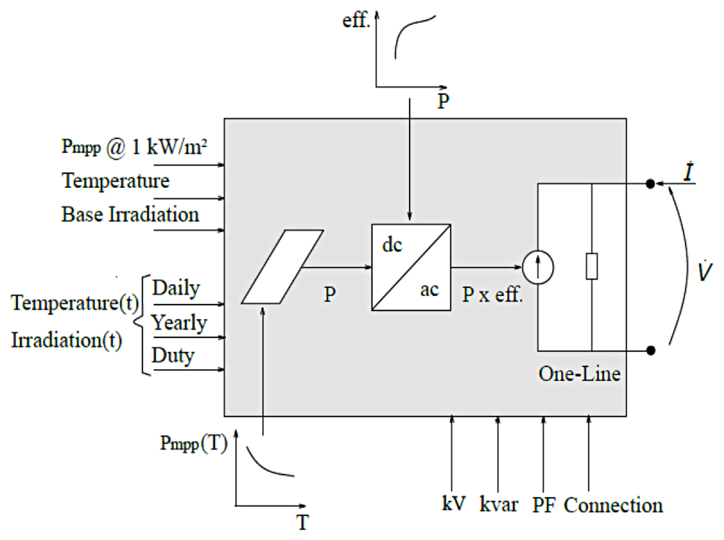
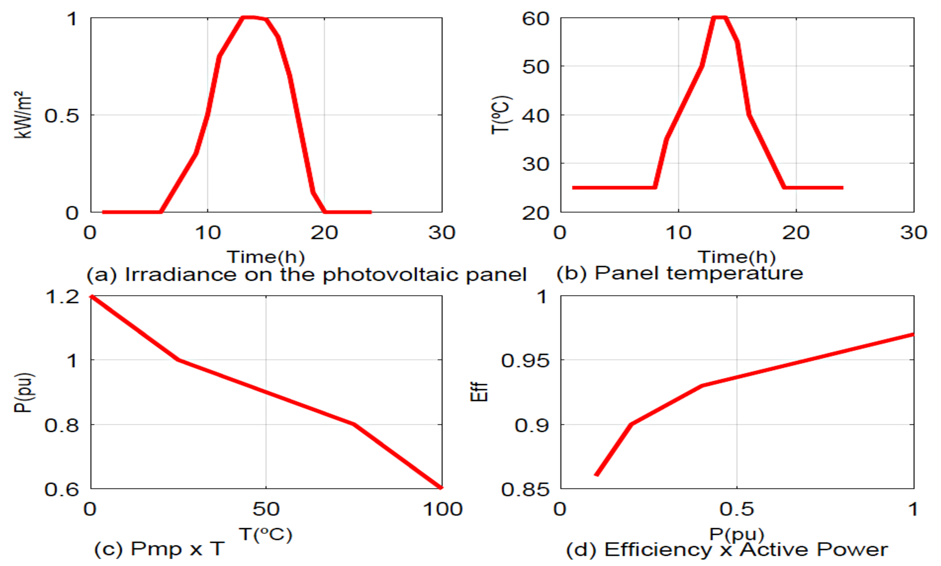
- P (t) = Pmpp(1kW/m2) × irrad(t) × irradBase × Pmpp(T (t))
- P(t): output power of the PV array at a specific time, t
- Pmpp(1 kW/m2): rated power at the maximum power point and a selected temperature
- irrad(t): per unit irradiation value at t
- irradBase: base irradiation value for shape multipliers
- Pmpp(T (t)): Pmpp correction factor as a function of the temperature at t
- eff (P (t)): inverter efficiency for a given P (t)
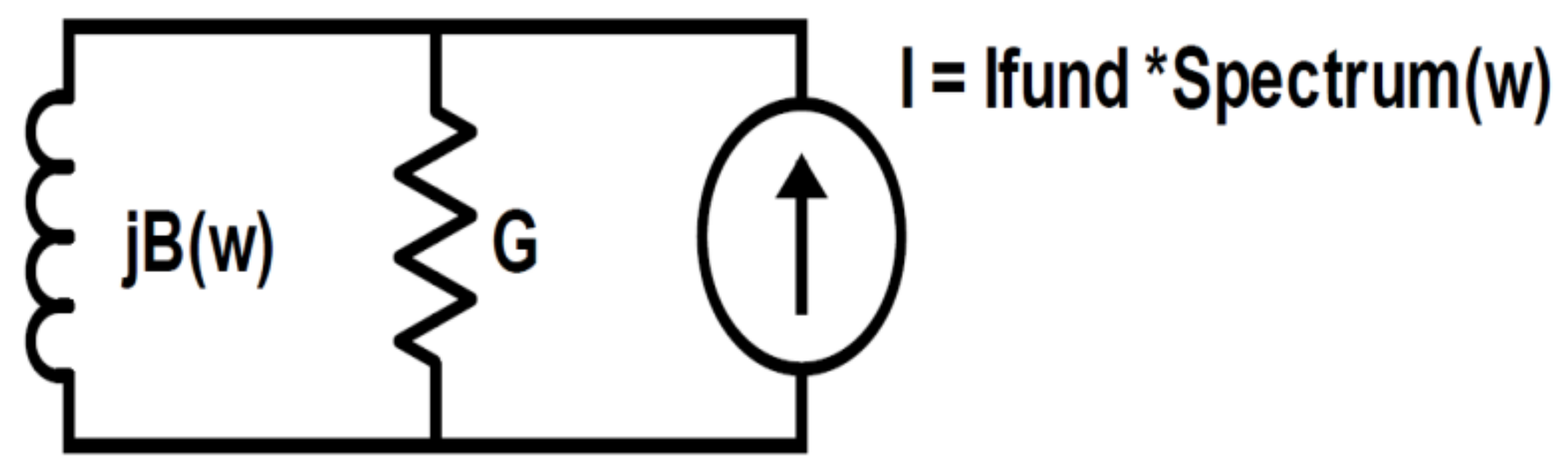
- Im—the vector of source currents
- Ym—nodal admittance matrix
- Vm—the vector of bus voltages
- m—harmonic order
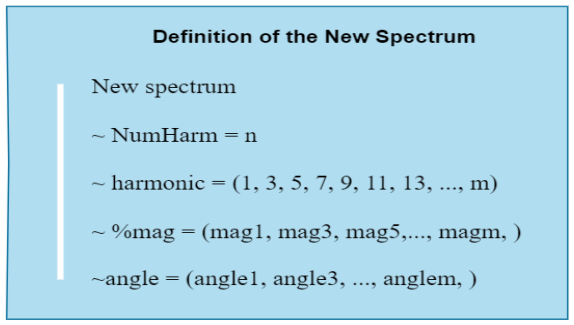
- New Spectrum—defines the specific name for the analysis
- NumHarm—specifies the number of harmonics in the spectrum
- Harmonic—specifies the harmonics of interest
- %mag—percentage magnitude relative to fundamental value
- Angle—angle of harmonic components
3. Results and Discussion
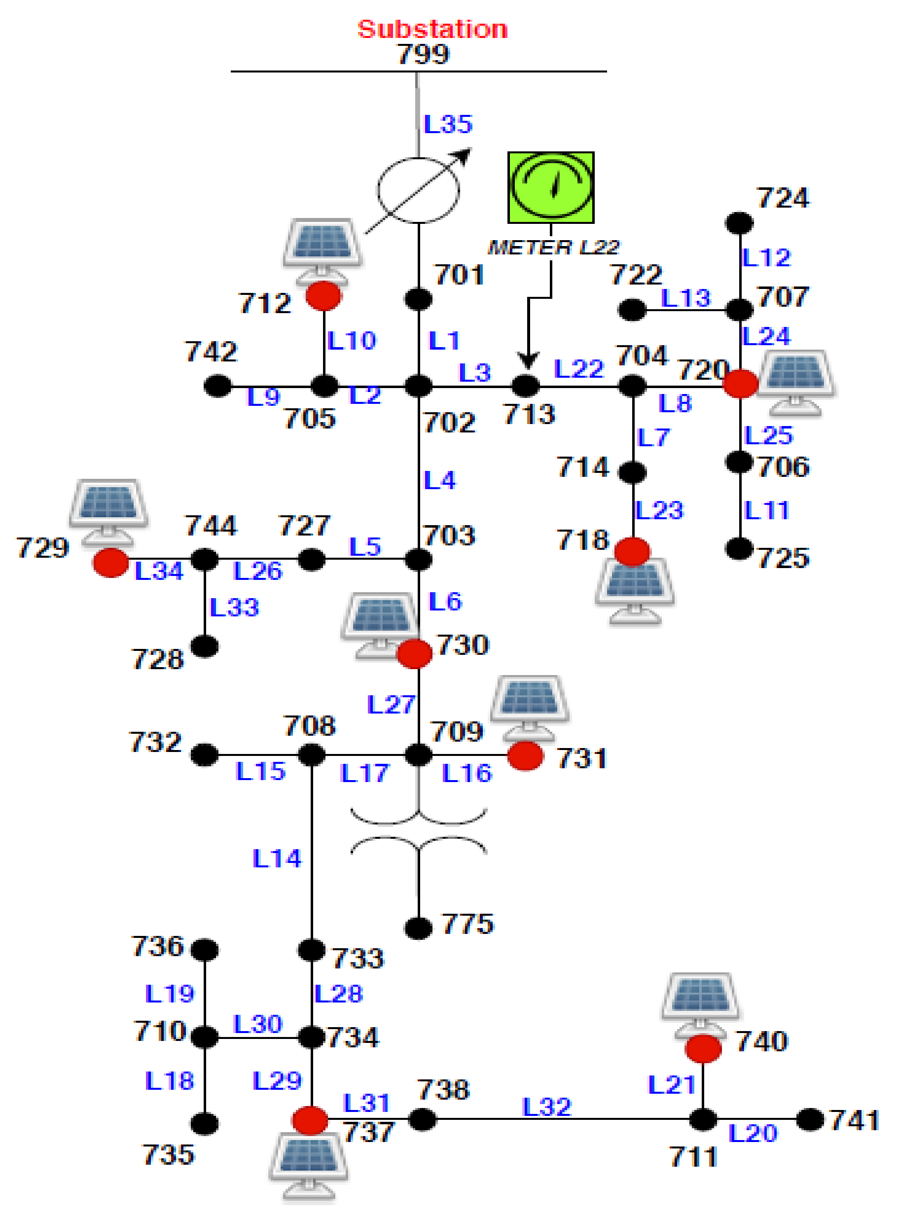
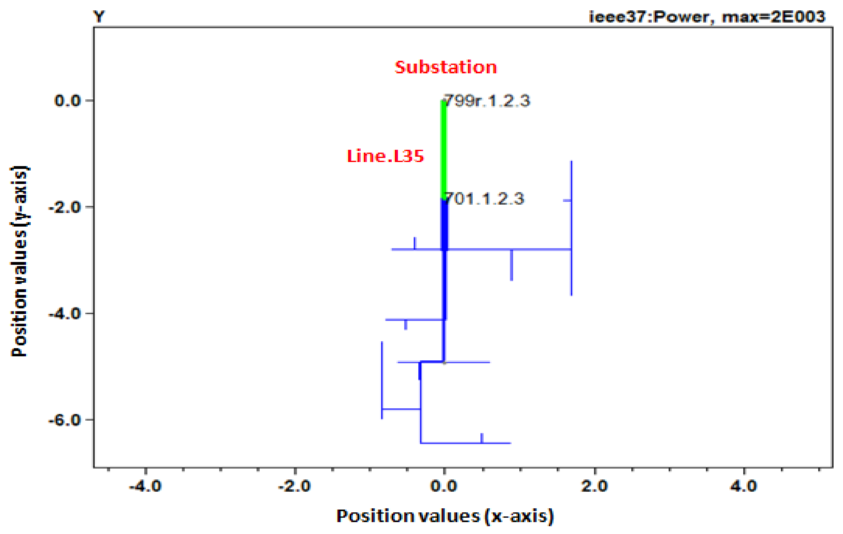
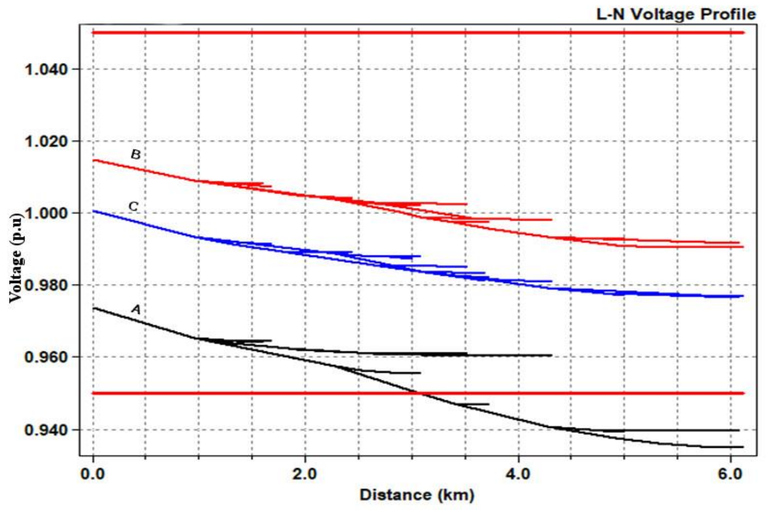
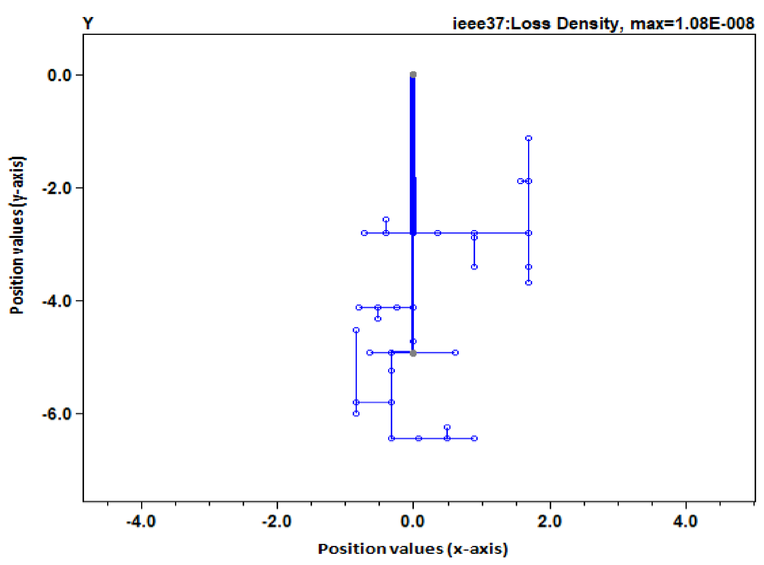
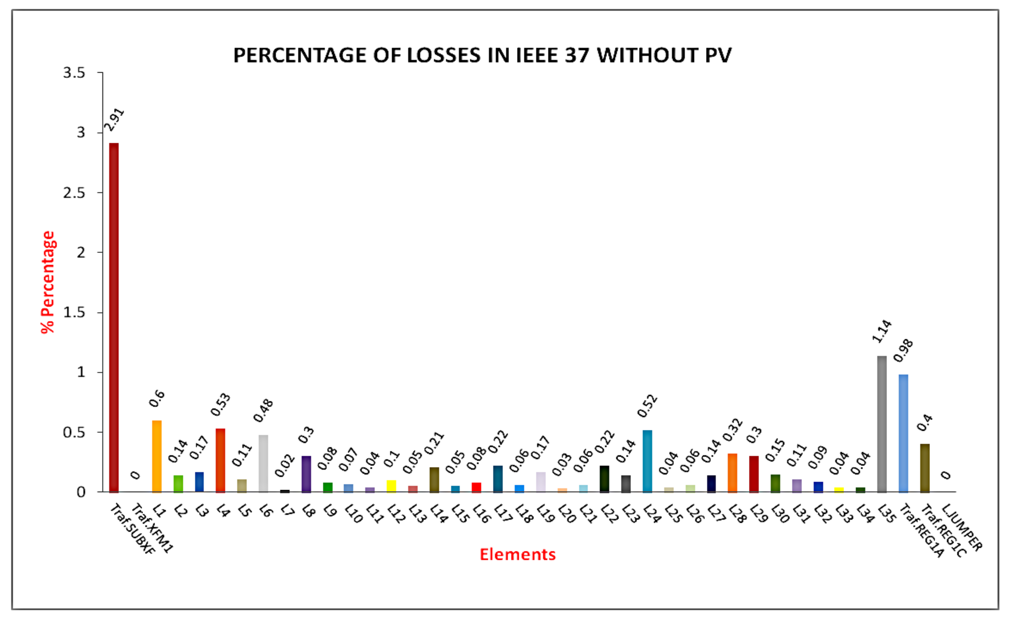
3.1. Case Study 1—System without Photovoltaic Generation
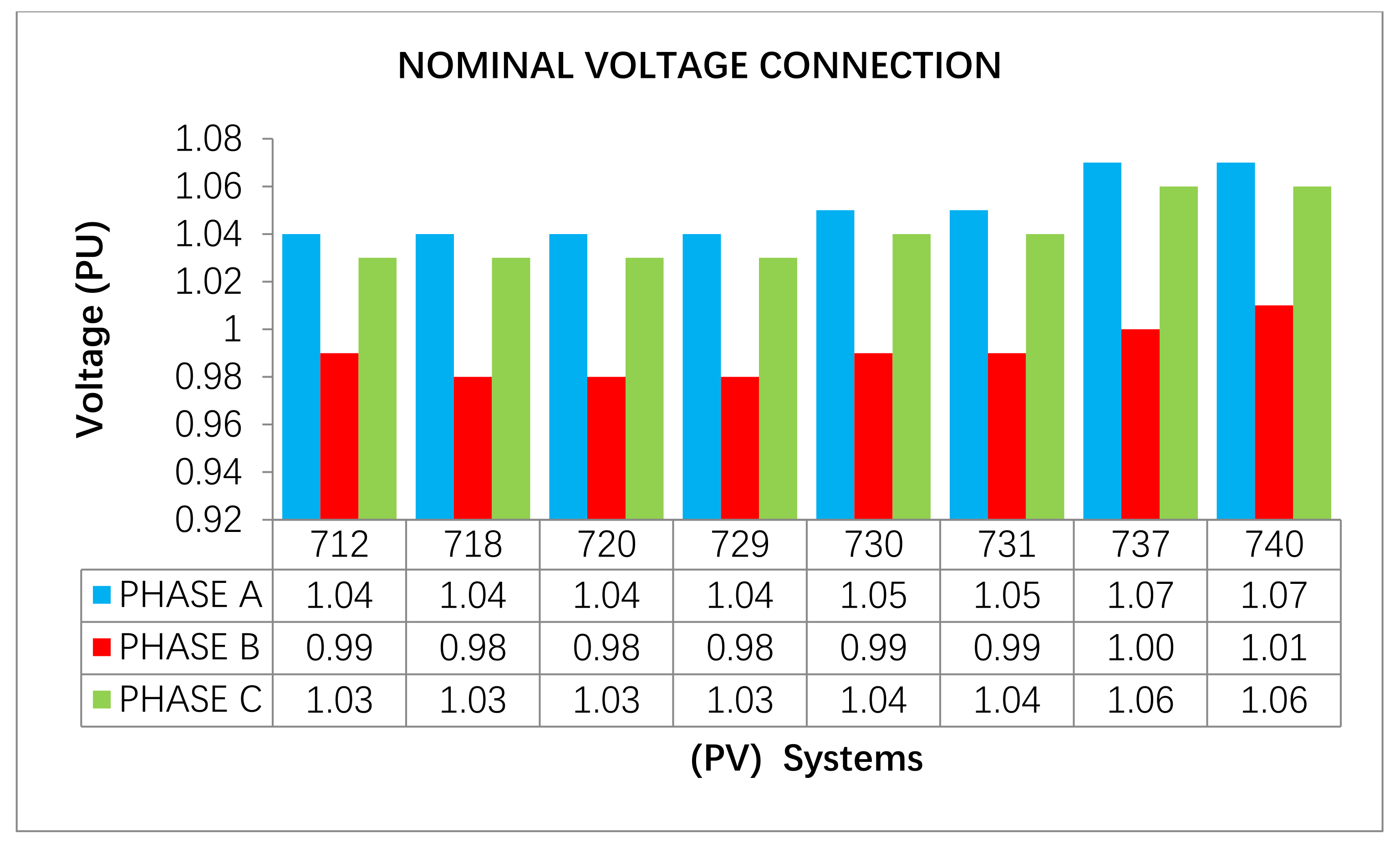
3.2. Case Study 2—System with Photovoltaic Generation
- New Spectrum.pv_harmonics numharm = 7
- harmonic = (1,3,5,7,9,11,13)
- %mag = (100,0.69,0.63,0.56,0.19,0.07,0.17)
- angle = (0,128,207,10,356,329,304)
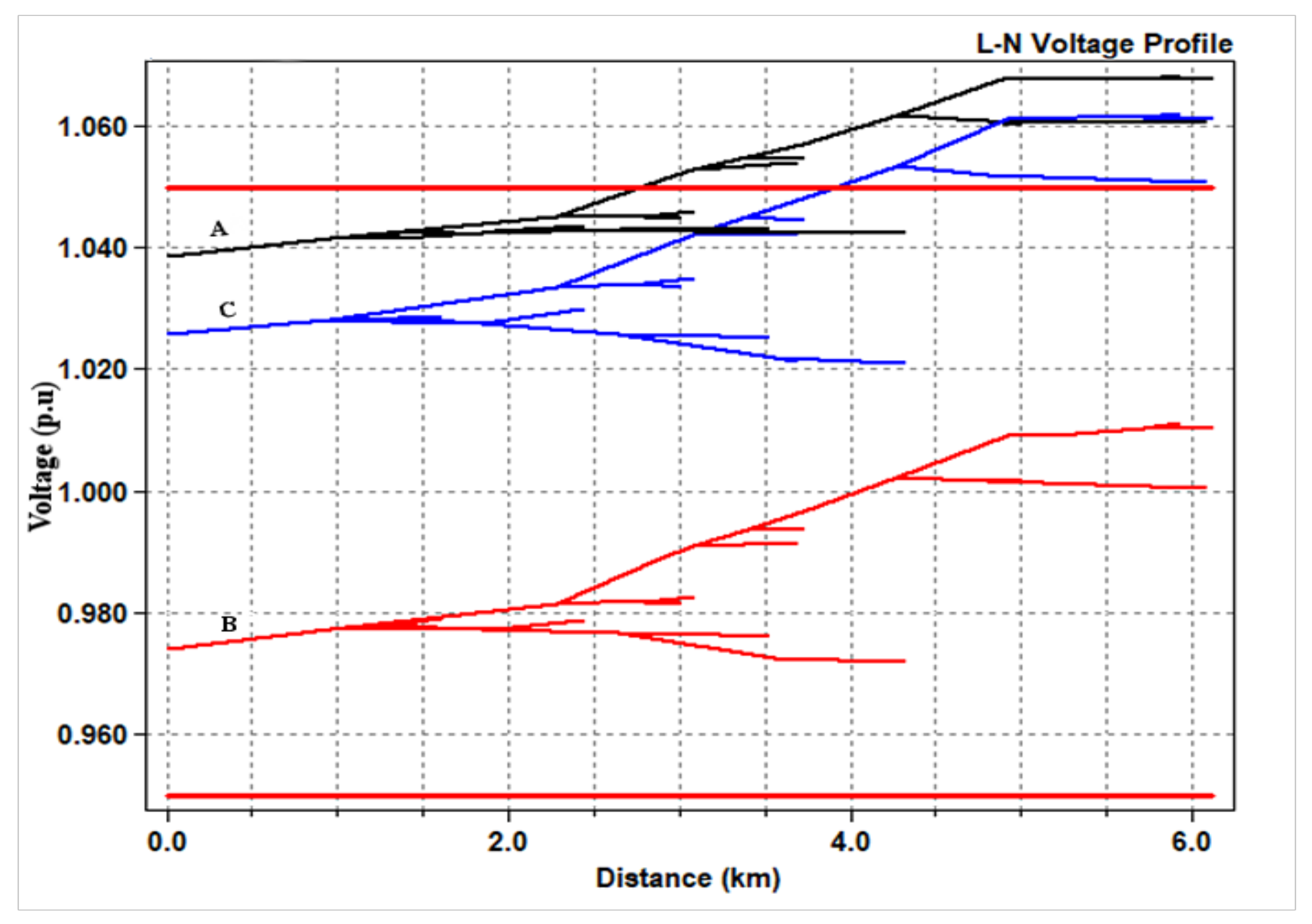
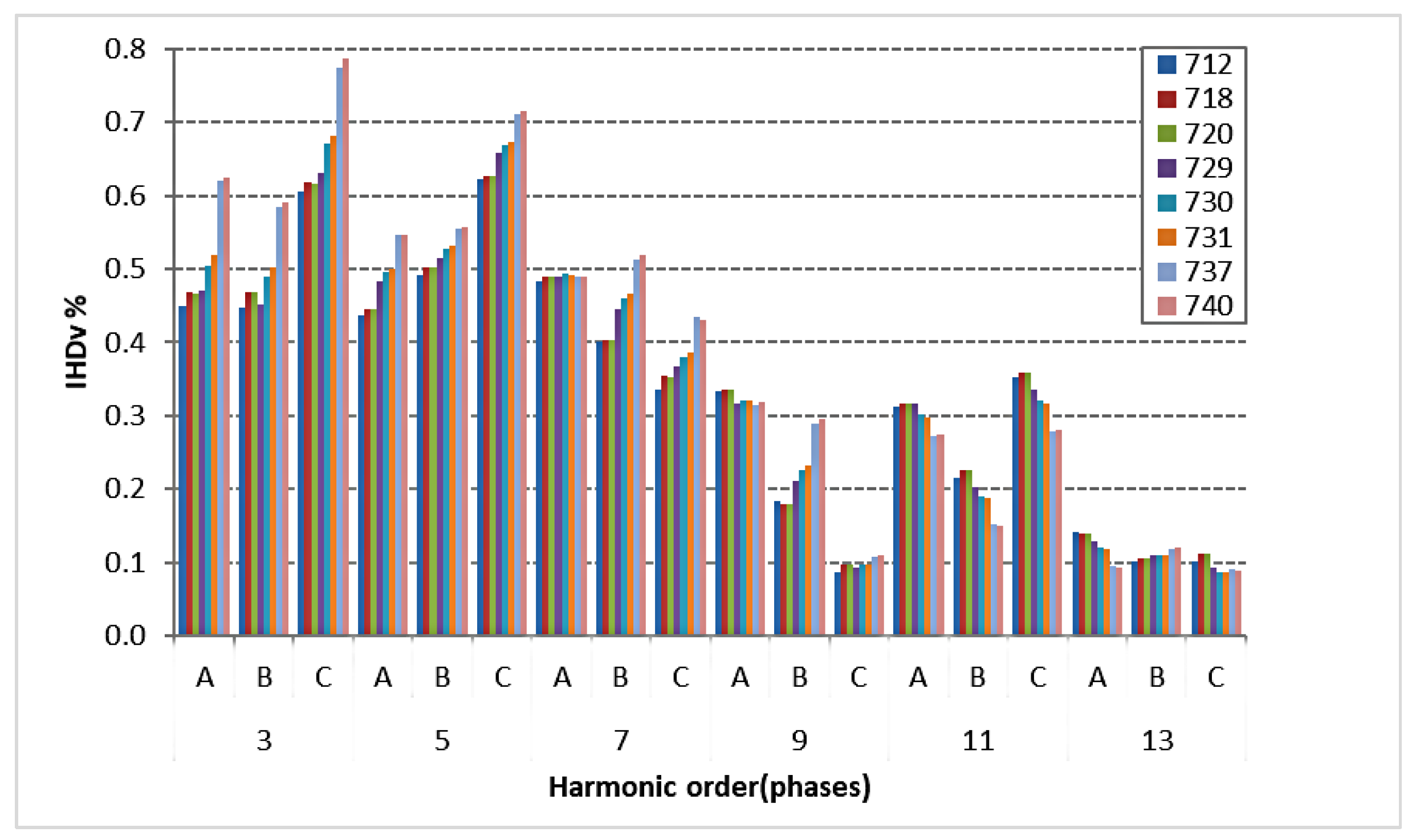
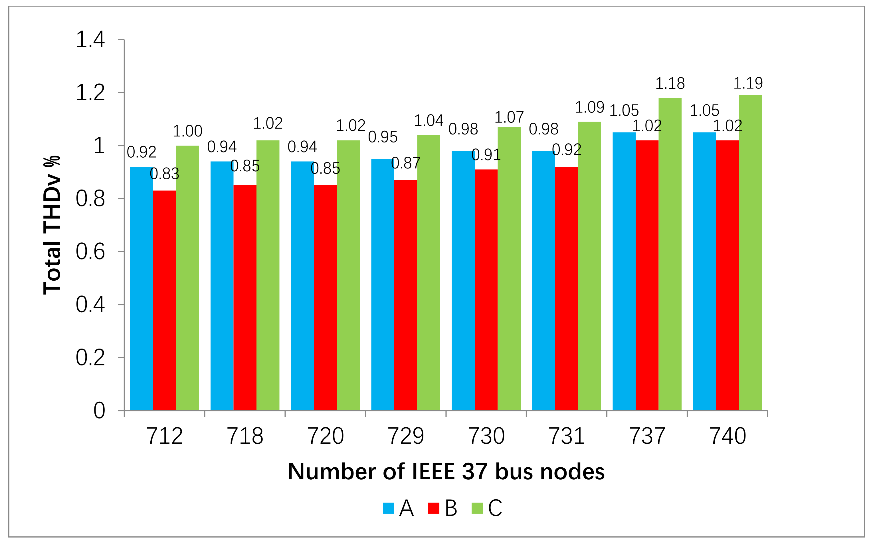
3.3. Analysis of Harmonic Voltages (IHDV and THDV)
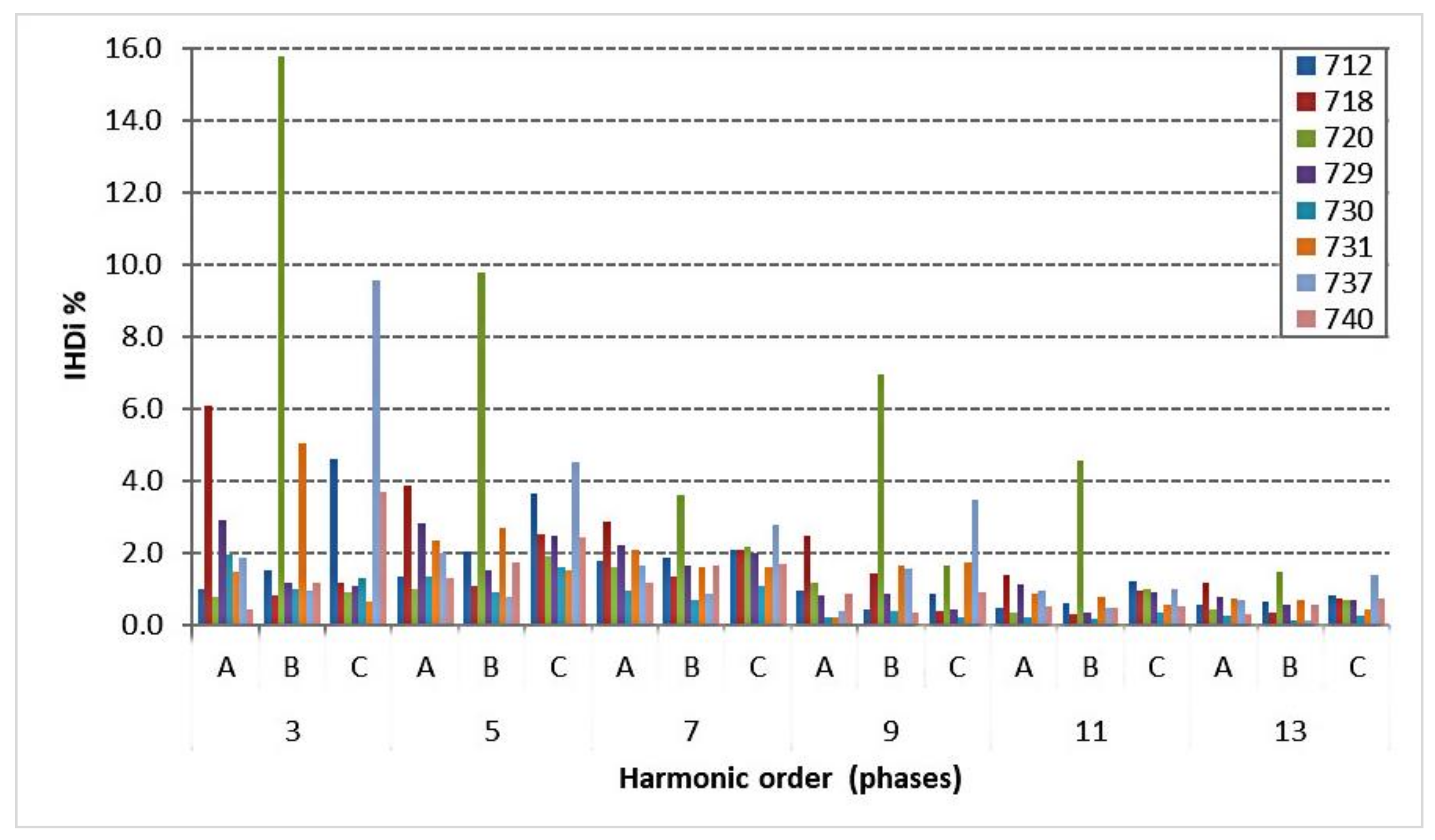
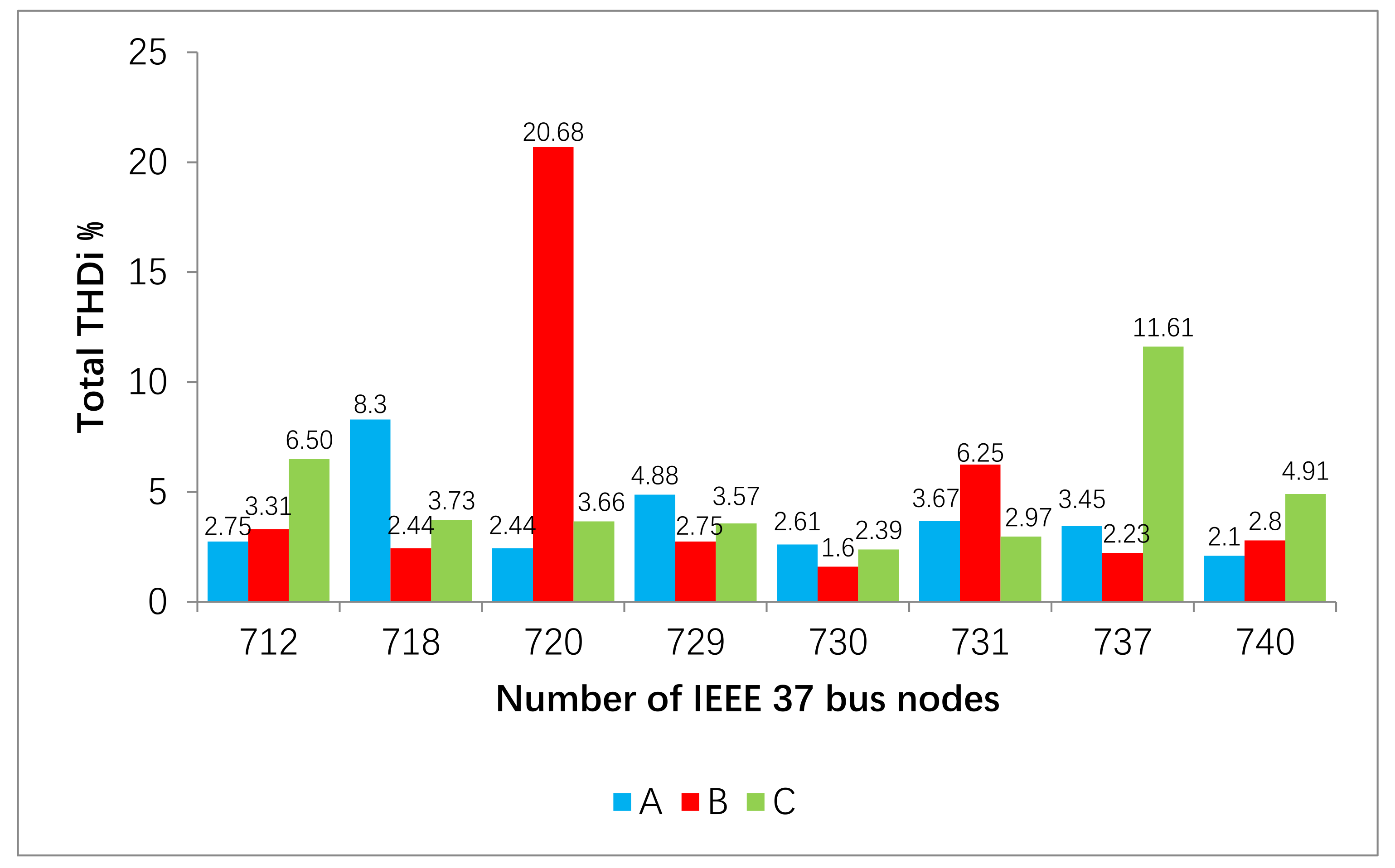
3.4. Analysis of Harmonic Currents (IHDI and THDI)
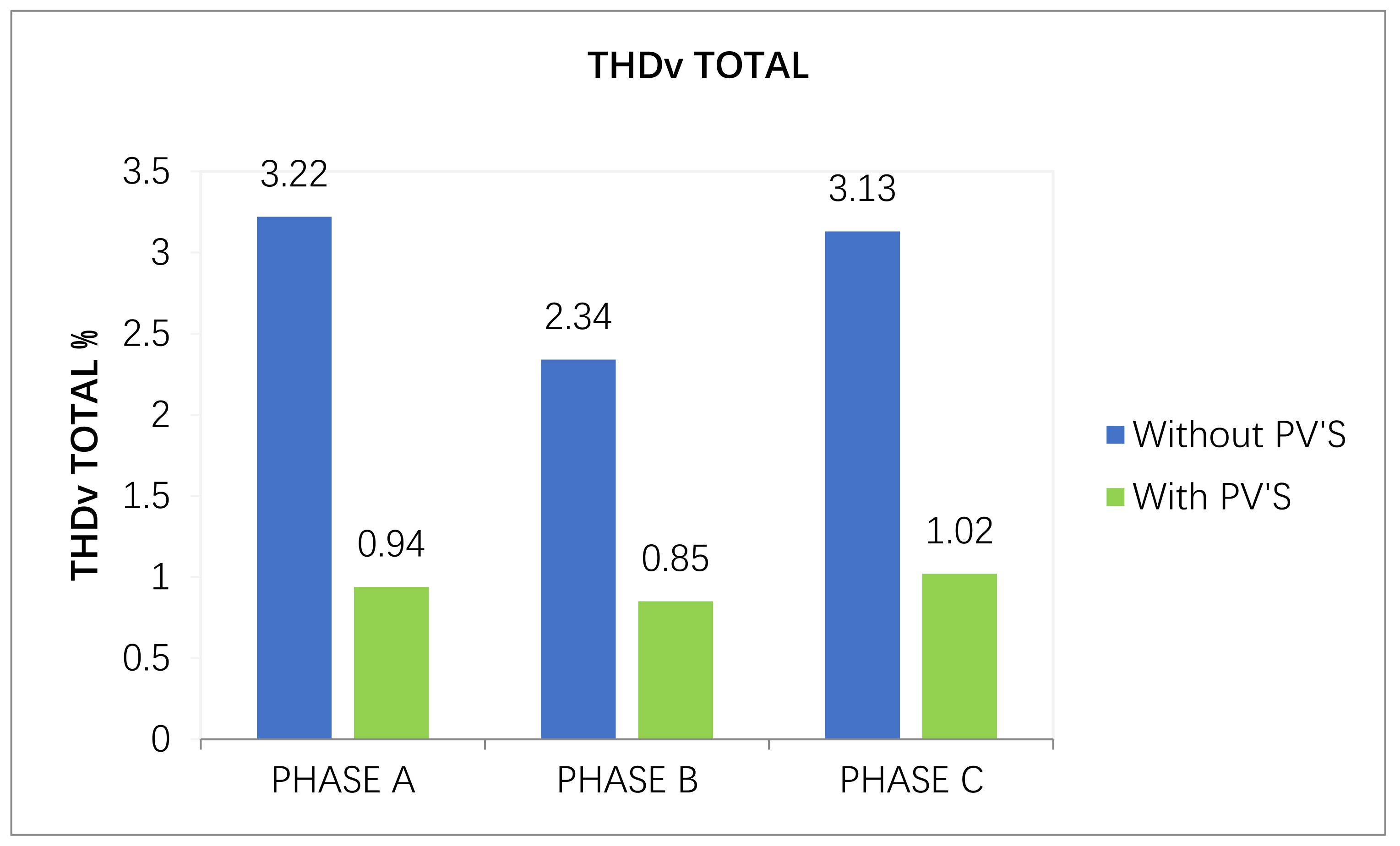
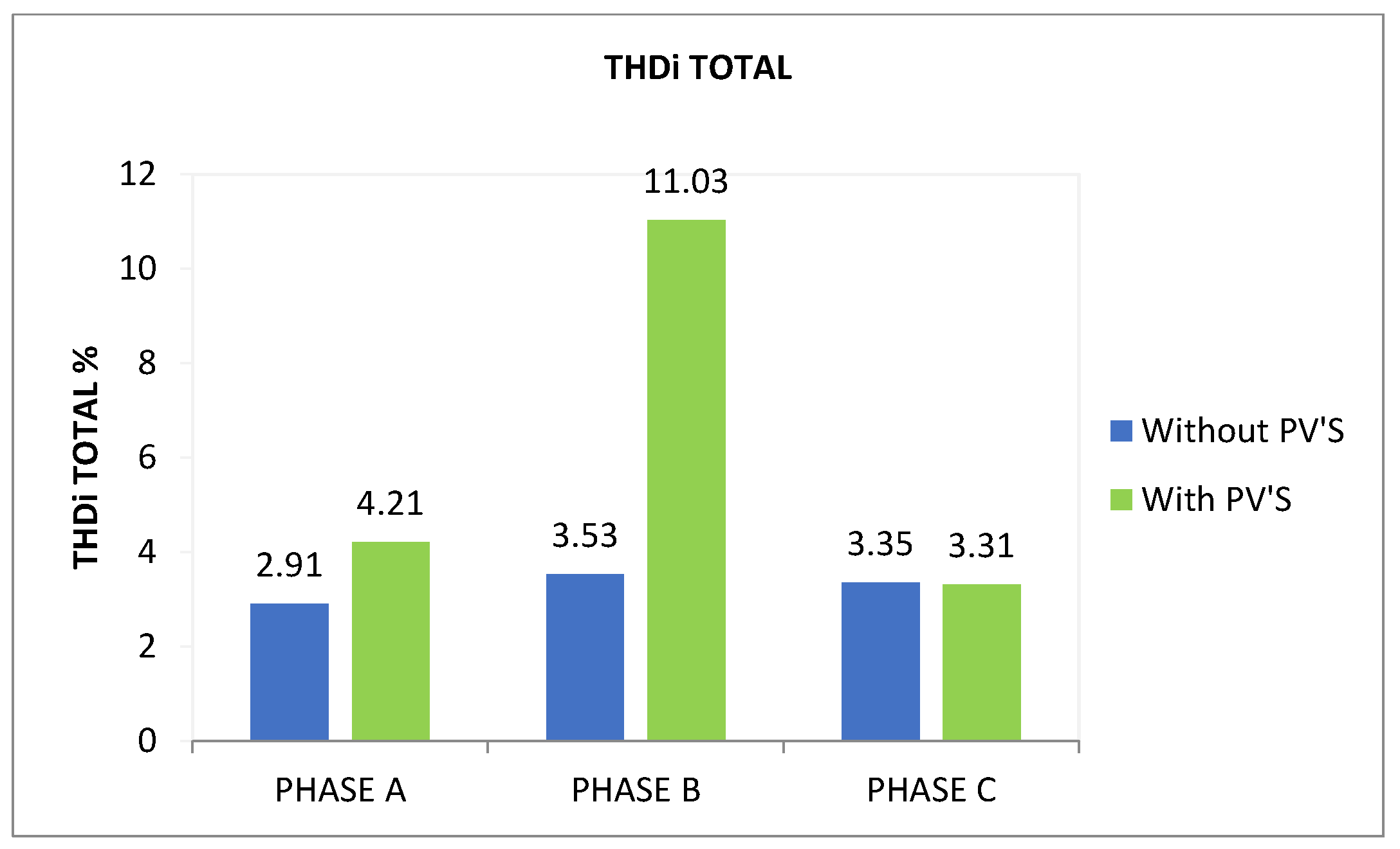
3.5. THDv and THDi Comparative Levels with the Presence and Absence of Photovoltaic Systems
4. Conclusions
Author Contributions
Funding
Data Availability Statement
Acknowledgments
Conflicts of Interest
References
- National Association of Clean Air Agencies (NACAA). Implementing EPA’s Clean Power Plan: A Menu of Options. Chapter 10. Reduce Losses in the Transmission and Distribution System; NACAA: Washington, DC, USA, 2015. [Google Scholar]
- Schinke, A.; Erlich, I. Enhanced voltage and frequency stability for power systems with high penetration of distributed photovoltaic generation. IFAC-Papercept 2018, 51, 31–36. [Google Scholar] [CrossRef]
- Ebad, M.; Grady, W.M. An approach for assessing high-penetration PV impact on distribution feeders. Electr. Power Syst. Res. 2016, 133, 347–354. [Google Scholar] [CrossRef]
- Anzalchi, A.; Sundararajan, A.; Moghadasi, A.; Sarwat, A. Power quality and voltage profile analyses of high penetration grid-tied photovoltaics: A case study. In 2017 IEEE Industry Applications Society Annual Meeting; IEEE: Cincinnati, OH, USA, 2017; pp. 1–8. [Google Scholar]
- Anurangi, R.O.; Rodrigo, A.S.; Jayatunga, U. Effects of high levels of harmonic penetration in distribution networks with photovoltaic inverters. In Proceedings of the 2017 IEEE International Conference on Industrial and Information Systems (ICIIS), Peradeniya, Sri Lanka, 15–16 December 2017; pp. 1–6. [Google Scholar]
- Barutcu, I.C.; Karatepe, E.; Boztepe, M. Impact of harmonic limits on PV penetration levels in unbalanced distribution networks considering load and irradiance uncertainty. Int. J. Electr. Power Energy Syst. 2020, 118, 105780. [Google Scholar] [CrossRef]
- Sinvula, R.; Abo-Al-Ez, K.M.; Kahn, M.T. Total harmonics distortion (THD) with PV System integration in smart grids: Case study. In Proceedings of the 2019 International Conference on the Domestic Use of Energy (DUE), Wellington, South Africa, 25–27 March 2019; pp. 102–108. [Google Scholar]
- Fang, W.; Huang, Q.; Huang, S.; Yang, J.; Meng, E.; Li, Y. Optimal sizing of utility-scale photovoltaic power generation complementarily operating with hydropower: A case study of the world’s largest hydro-photovoltaic plant. Energy Convers. Manag. 2017, 136, 161–172. [Google Scholar] [CrossRef]
- Colmenar-Santos, A.; Linares-Mena, A.-R.; Molina-Ibáñez, E.L.; Rosales-Asensio, E.; Borge-Diez, D. Technical challenges for the optimum penetration of grid-connected photovoltaic systems: Spain as a case study. Renew. Energy 2020, 145, 2296–2305. [Google Scholar] [CrossRef]
- Kerdoum, P.; Premrudeepreechacharn, S. Analysis of PV penetration level on low voltage system in Chiang Mai Thailand. Energy Rep. 2020, 6, 754–760. [Google Scholar] [CrossRef]
- Kyritsis, A.; Voglitsis, D.; Papanikolaou, N.; Tselepis, S.; Christodoulou, C.; Gonos, I.; Kalogirou, S.A. Evolution of PV systems in Greece and review of applicable solutions for higher penetration levels. Renew. Energy 2017, 109, 487–499. [Google Scholar] [CrossRef]
- Pereira, H.A.; Freijedo, F.D.; Silva, M.M.; Mendes, V.F.; Teodorescu, R. Harmonic current prediction by impedance modeling of grid-tied inverters: A 1.4MW PV plant case study. Int. J. Electr. Power Energy Syst. 2017, 93, 30–38. [Google Scholar] [CrossRef]
- Seme, S.; Lukač, N.; Štumberger, B.; Hadžiselimović, M. Power quality experimental analysis of grid-connected photovoltaic systems in urban distribution networks. Energy 2017, 139, 1261–1266. [Google Scholar] [CrossRef]
- McBee, K.D. Transformer aging due to high penetrations of PV, EV charging, and energy storage applications. In Proceedings of the 2017 Ninth Annual IEEE Green Technologies Conference (GreenTech), Denver, CO, USA, 29–31 March 2017; pp. 163–170. [Google Scholar]
- Sakar, S.; Balci, M.E.; Abdel Aleem, S.H.E.; Zobaa, A.F. Increasing PV hosting capacity in distorted distribution systems using passive harmonic filtering. Electr. Power Syst. Res. 2017, 148, 74–86. [Google Scholar] [CrossRef] [Green Version]
- Srinath, S.; Poongothai, M.S.; Aruna, T. PV integrated shunt active filter for harmonic compensation. Energy Procedia 2017, 117, 1134–1144. [Google Scholar] [CrossRef]
- Patsalides, M.; Efthymiou, V.; Stavrou, A.; Georghiou, G.E. A generic transient PV system model for power quality studies. Renew. Energy 2016, 89, 526–542. [Google Scholar] [CrossRef]
- Alhafadhi, L.; Teh, J. Advances in reduction of total harmonic distortion in solar photovoltaic systems: A literature review. Int. J. Energy Res. 2020, 44, 2455–2470. [Google Scholar] [CrossRef]
- Kopicka, M.; Ptacek, M.; Toman, P. Analysis of the power quality and the impact of photovoltaic power plant operation on low-voltage distribution network. In Proceedings of the 2014 Electric Power Quality and Supply Reliability Conference (PQ), Rakvere, Estonia, 11–13 June 2014; pp. 99–102. [Google Scholar]
- Osma-Pinto, G.; García-Rodríguez, M.; Moreno-Vargas, J.; Duarte-Gualdrón, C. Impact evaluation of grid-connected PV systems on PQ parameters by comparative analysis based on inferential statistics. Energies 2020, 13, 1668. [Google Scholar] [CrossRef] [Green Version]
- Abas, N.; Dilshad, S.; Khalid, A.; Saleem, M.S.; Khan, N. Power quality improvement using dynamic voltage restorer. IEEE Access 2020, 8, 164325–164339. [Google Scholar] [CrossRef]
- Zare, F.; Soltani, H.; Kumar, D.; Davari, P.; Delpino, H.A.M.; Blaabjerg, F. Harmonic emissions of three-phase diode rectifiers in distribution networks. IEEE Access 2017, 5, 2819–2833. [Google Scholar] [CrossRef]
- Sinvula, R.; Abo-Al-Ez, K.M.; Kahn, M.T. Harmonic source detection methods: A systematic literature review. IEEE Access 2019, 7, 74283–74299. [Google Scholar] [CrossRef]
- Macêdo, W.N.; Zilles, R. Influence of the power contribution of a grid-connected photovoltaic system and its operational particularities. Energy Sustain. Dev. 2009, 13, 202–211. [Google Scholar] [CrossRef]
- Chidurala, A. High Penetration of PV Systems in Low Voltage Distribution Networks: Investigation of Power Quality Challenges and Mitigation. Ph.D. Thesis, School of Information Technology and Electrical Engineering, The University of Queensland, Brisbane, Australia, 2016. [Google Scholar]
- Zhang, J.; Isobe, T.; Tadano, H. Model-based control for grid-tied inverters operated in discontinuous current mode with low harmonic current distortion. IEEE Trans. Power Electron. 2020, 35, 11167–11180. [Google Scholar] [CrossRef]
- Chidurala, A.; Kumar Saha, T.; Mithulananthan, N. Harmonic impact of high penetration photovoltaic system on unbalanced distribution networks–learning from an urban photovoltaic network. IET Renew. Power Gener. 2016, 10, 485–494. [Google Scholar] [CrossRef]
- Schlabbach, J.; Grob, A.; Chicco, G. Influence of harmonic system voltages on the harmonic current emission of photovoltaic inverters. In Proceedings of the 2007 International Conference on Power Engineering, Energy and Electrical Drives, Setubal, Portugal, 12–14 April 2007; pp. 545–550. [Google Scholar] [CrossRef]
- Kouveliotis-Lysikatos, I.; Kotsampopoulos, P.; Hatziargyriou, N. Harmonic Study in LV Networks with high penetration of PV systems. In Proceedings of the 2015 IEEE Eindhoven PowerTech, Cluj-Napoca, Romania, 29 June–2 July 2015; pp. 1–6. [Google Scholar]
- Pereira, C.A.N.; Lopes, J.A.P.; Matos, M.A.C.C. Assessment of the distributed generation hosting capacity incorporating harmonic distortion limits. In Proceedings of the 2018 International Conference on Smart Energy Systems and Technologies (SEST), Seville, Spain, 10–12 September 2018; pp. 1–6. [Google Scholar]
- Awadallah, M.A.; Venkatesh, B.; Singh, B.N. Impact of solar panels on power quality of distribution networks and transformers. Can. J. Electr. Comput. Eng. 2015, 38, 45–51. [Google Scholar] [CrossRef]
- Kharrazi, A.; Sreeram, V.; Mishra, Y. Assessment techniques of the impact of grid-tied rooftop photovoltaic generation on the power quality of low voltage distribution network-A review. Renew. Sustain. Energy Rev. 2020, 120, 109643. [Google Scholar] [CrossRef]
- Patsalides, M.; Evagorou, D.; Makrides, G.; Achillides, Z.; Georghiou, G.E.; Stavrou, A.; Werner, J.H. The effect of solar irradiance on the power quality behaviour of grid connected photovoltaic systems. Int. Conf. Renew. Energy Power Qual. 2007, 1, 323–330. [Google Scholar] [CrossRef]
- Chicco, G.; Schlabbach, J.; Spertino, F. Experimental assessment of the waveform distortion in grid-connected photovoltaic installations. Sol. Energy 2009, 83, 1026–1039. [Google Scholar] [CrossRef]
- Rajapakse, A.D.; Muthumuni, D. Simulation tools for photovoltaic system grid integration studies. In Proceedings of the 2009 IEEE Electrical Power & Energy Conference (EPEC), Montreal, QC, Canada, 22–23 October 2009; pp. 1–5. [Google Scholar]
- Sa’ed, J.A.; Quraan, M.; Samara, Q.; Favuzza, S.; Zizzo, G. Impact of integrating photovoltaic based DG on distribution network harmonics. In Proceedings of the 2017 IEEE International Conference on Environment and Electrical Engineering and 2017 IEEE Industrial and Commercial Power Systems Europe (EEEIC/I&CPS Europe), Milan, Italy, 6–9 June 2017; pp. 1–5. [Google Scholar]
- Dugan, R.C.; Montenegro, D. Reference Guide: The Open Distribution System Simulator (OpenDSS); Electric Power Research Institute (EPRI), Inc: Washington, DC, USA, 2019. [Google Scholar]
- IEEE Power & Energy Society (IEEE PES AMPS DSAS Test Feeder Working Group). Available online: https://site.ieee.org/pes-testfeeders/ (accessed on 15 March 2020).
- Dugan, R.C. Reference Guide: OpenDSS PVSystem Element Model; Electric Power Research Institute (EPRI), Inc.: Washington, DC, USA, 2019. [Google Scholar]
- National Electrical Manufacturers Association. American National Standards Institute (ANSI) C84.1-2006, Voltage Ratings for Electric Power Systems and Equipment, Power Quality; NEMA: Rosslyn, VA, USA, 2006. [Google Scholar]
- Institute of Electrical and Electronics Engineers (IEEE). IEEE Recommended Practice and Requirements for Harmonic Control in Electric Power Systems-Redline in IEEE Std 519-2014 (Revision of IEEE Std 519-1992)-Redline; IEEE: New York, NY, USA, 2014. [Google Scholar]


| Location of PV Plants | Generation Capacity |
|---|---|
| 737 | 2 MW |
| 740 | 350 kW |
| 712 | 350 kW |
| 718 | 350 kW |
| 729 | 350 kW |
| 730 | 350 kW |
| 731 | 350 kW |
| 720 | 350 kW |
| Element | Phase | kW | kvar | kVA | PF * |
|---|---|---|---|---|---|
| Transf.SUBXF | A | 731.8 | 630.8 | 966.1 | 0.76 |
| Transf.SUBXF | B | 836.0 | 357.4 | 909.2 | 0.92 |
| Transf.SUBXF | C | 1020.7 | 584.4 | 1176.1 | 0.87 |
| TOTAL CONVENTIONAL GENERATION ELEMENT | 2588.5 | 1572.6 | 3028.7 | 0.85 |
| Attendance Voltage (AT) | Range of Variation in pu |
|---|---|
| Adequate | 0.95 ≤ v ≤ 1.05 pu |
| Poor | 0.90 ≤ v < 0.95 pu |
| Critical | <0.90 pu or >1.05 pu |
| Element | Losses (kW) | %Power | (kvar) |
|---|---|---|---|
| Transformer.SUBXF | 75.44 | 2.91 | 301.77 |
| Transformer.XFM1 | 0.00 | 0.00 | 0.00 |
| Line.L1 | 10.96 | 0.60 | 10.81 |
| Line.L2 | 0.25 | 0.14 | −0.02 |
| Line.L3 | 0.92 | 0.17 | 0.41 |
| Line.L4 | 5.93 | 0.53 | 5.41 |
| Line.L5 | 0.28 | 0.11 | 0.03 |
| Line.L6 | 4.08 | 0.48 | 2.20 |
| Line.L7 | 0.03 | 0.02 | −0.01 |
| Line.L8 | 0.98 | 0.30 | 0.30 |
| Line.L9 | 0.08 | 0.08 | −0.06 |
| Line.L10 | 0.06 | 0.07 | −0.04 |
| Line.L11 | 0.02 | 0.04 | −0.07 |
| Line.L12 | 0.04 | 0.10 | −0.18 |
| Line.L13 | 0.08 | 0.05 | −0.00 |
| Line.L14 | 1.36 | 0.21 | 0.68 |
| Line.L15 | 0.02 | 0.05 | −0.07 |
| Line.L16 | 0.07 | 0.08 | −0.15 |
| Line.L17 | 1.54 | 0.22 | 0.80 |
| Line.L18 | 0.05 | 0.06 | −0.03 |
| Line.L19 | 0.07 | 0.17 | −0.30 |
| Line.L20 | 0.01 | 0.03 | −0.12 |
| Line.L21 | 0.05 | 0.06 | −0.03 |
| Line.L22 | 0.98 | 0.22 | 0.38 |
| Line.L23 | 0.11 | 0.14 | −0.10 |
| Line.L24 | 1.06 | 0.52 | 0.09 |
| Line.L25 | 0.02 | 0.04 | −0.18 |
| Line.L26 | 0.12 | 0.06 | −0.02 |
| Line.L27 | 1.11 | 0.14 | 0.58 |
| Line.L28 | 1.78 | 0.32 | 0.87 |
| Line.L29 | 1.14 | 0.30 | 0.45 |
| Line.L30 | 0.19 | 0.15 | −0.06 |
| Line.L31 | 0.29 | 0.11 | 0.05 |
| Line.L32 | 0.12 | 0.09 | −0.05 |
| Line.L33 | 0.05 | 0.04 | −0.03 |
| Line.L34 | 0.02 | 0.04 | −0.07 |
| Line.L35 | 28.44 | 1.14 | 26.87 |
| Transformer.REG1A | 7.61 | 0.98 | 19.03 |
| Transformer.REG1C | 6.97 | 0.40 | 17.44 |
| Line.JUMPER | 0.00 | 0.00 | 0.00 |
| Line losses = 62.3 kW | |||
| Transformer losses = 90.0 kW | |||
| Total losses = 152.3 kW | |||
| Total load power = 2436.0 kW | |||
| Percent losses for circuit = 6.25% | |||
| Element | Phase | kW | kvar | kVA | PF |
|---|---|---|---|---|---|
| Transformer.SUBXF | A | 656.5 | 722.6 | 976.3 | 0.67 |
| Transformer.SUBXF | B | 628.6 | 315.3 | 703.2 | 0.89 |
| Transformer.SUBXF | C | 289.8 | 543.1 | 615.6 | 0.47 |
| Total conventional generation | 1574.9 | 1581.0 | 2231.6 | 0.70 | |
| PVSystem.PV1 | A | 110.7 | 0.0 | 110.7 | 1 |
| PVSystem.PV1 | B | 110.7 | 0.0 | 110.7 | 1 |
| PVSystem.PV1 | C | 110.8 | 0.0 | 110.8 | 1 |
| Total | 332.2 | 0.0 | 332.2 | 1 | |
| PVSystem.PV2 | A | 632.8 | 0.0 | 632.8 | 1 |
| PVSystem.PV2 | B | 632.8 | 0.0 | 632.8 | 1 |
| PVSystem.PV2 | C | 632.9 | 0.0 | 632.9 | 1 |
| Total | 1898.5 | 0.0 | 1898.5 | 1 | |
| PVSystem.PV3 | A | 110.7 | 0.0 | 110.7 | 1 |
| PVSystem.PV3 | B | 110.8 | 0.0 | 110.8 | 1 |
| PVSystem.PV3 | C | 110.8 | 0.0 | 110.8 | 1 |
| Total | 332.3 | 0.0 | 332.3 | 1 | |
| PVSystem.PV4 | A | 110.7 | 0.0 | 110.7 | 1 |
| PVSystem.PV4 | B | 110.7 | 0.0 | 110.7 | 1 |
| PVSystem.PV4 | C | 110.8 | 0.0 | 110.8 | 1 |
| Total | 332.2 | 0.0 | 332.2 | 1 | |
| PVSystem.PV5 | A | 110.7 | 0.0 | 110.7 | 1 |
| PVSystem.PV5 | B | 110.7 | 0.0 | 110.7 | 1 |
| PVSystem.PV5 | C | 110.8 | 0.0 | 110.8 | 1 |
| Total | 332.2 | 0.0 | 332.2 | 1 | |
| PVSystem.PV6 | A | 110.7 | 0.0 | 110.7 | 1 |
| PVSystem.PV6 | B | 110.8 | 0.0 | 110.8 | 1 |
| PVSystem.PV6 | C | 110.8 | 0.0 | 110.8 | 1 |
| Total | 332.3 | 0.0 | 332.3 | 1 | |
| PVSystem.PV7 | A | 110.7 | 0.0 | 110.7 | 1 |
| PVSystem.PV7 | B | 110.7 | 0.0 | 110.7 | 1 |
| PVSystem.PV7 | C | 110.8 | 0.0 | 110.8 | 1 |
| Total | 332.2 | 0.0 | 332.2 | 1 | |
| PVSystem.PV8 | A | 110.7 | 0.0 | 110.7 | 1 |
| PVSystem.PV8 | B | 110.8 | 0.0 | 110.8 | 1 |
| PVSystem.PV8 | C | 110.8 | 0.0 | 110.8 | 1 |
| Total | 332.3 | 0.0 | 332.3 | 1 | |
| Total photovoltaic generation | 4224.2 | 0.0 | 4224.2 | 1 | |
| Total delivered | 5799.1 | 1581.0 | 6010.8 | 0.89 |
| Element | Losses (kW) | % Power | (kvar) |
|---|---|---|---|
| Transformer.SUBXF | 43.86 | 2.79 | 175.45 |
| Transformer.XFM1 | 0.00 | 0.00 | 0.00 |
| Line.L1 | 15.13 | 0.67 | 15.31 |
| Line.L2 | 0.19 | 0.13 | −0.05 |
| Line.L3 | 0.24 | 0.21 | 0.03 |
| Line.L4 | 15.09 | 0.75 | 15.10 |
| Line.L5 | 0.09 | 0.12 | −0.04 |
| Line.L6 | 16.41 | 0.84 | 8.83 |
| Line.L7 | 0.06 | 0.03 | −0.00 |
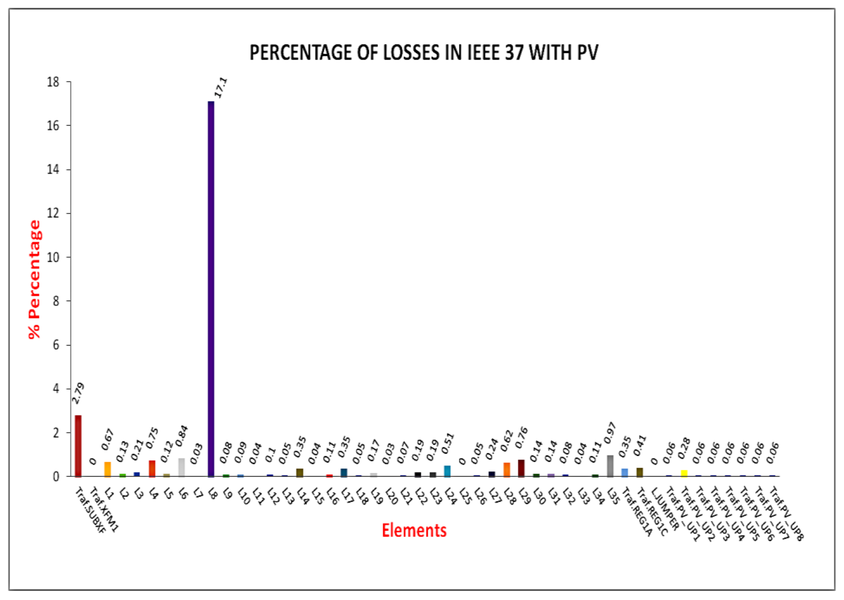
| Line.L8 | 0.38 | 17.10 | −0.04 |
| Line.L9 | 0.08 | 0.08 | −0.06 |
| Line.L10 | 0.22 | 0.09 | 0.00 |
| Line.L11 | 0.02 | 0.04 | −0.07 |
| Line.L12 | 0.04 | 0.10 | −0.19 |
| Line.L13 | 0.08 | 0.05 | −0.01 |
| Line.L14 | 5.38 | 0.35 | 2.84 |
| Line.L15 | 0.02 | 0.04 | −0.08 |
| Line.L16 | 0.26 | 0.11 | −0.05 |
| Line.L17 | 5.18 | 0.35 | 2.72 |
| Line.L18 | 0.04 | 0.05 | −0.04 |
| Line.L19 | 0.08 | 0.17 | −0.34 |
| Line.L20 | 0.01 | 0.03 | −0.14 |
| Line.L21 | 0.18 | 0.07 | −0.00 |
| Line.L22 | 0.38 | 0.19 | 0.06 |
| Line.L23 | 0.46 | 0.19 | 0.00 |
| Line.L24 | 1.06 | 0.51 | 0.08 |
| Line.L25 | 0.02 | 0.04 | −0.19 |
| Line.L26 | 0.06 | 0.05 | −0.06 |
| Line.L27 | 4.21 | 0.24 | 2.26 |
| Line.L28 | 10.17 | 0.62 | 5.40 |
| Line.L29 | 13.79 | 0.76 | 7.44 |
| Line.L30 | 0.18 | 0.14 | −0.09 |
| Line.L31 | 0.11 | 0.14 | −0.08 |
| Line.L32 | 0.17 | 0.08 | −0.05 |
| Line.L33 | 0.05 | 0.04 | −0.04 |
| Line.L34 | 0.30 | 0.11 | 0.02 |
| Line.L35 | 15.83 | 0.97 | 15.67 |
| Transformer.REG1A | 4.53 | 0.35 | 11.32 |
| Transformer.REG1C | 1.57 | 0.41 | 3.92 |
| Line.JUMPER | 0.00 | 0.00 | 0.00 |
| Transformer.PV_UP1 | 0.21 | 0.06 | 3.02 |
| Transformer.PV_UP2 | 5.26 | 0.28 | 75.60 |
| Transformer.PV_UP3 | 0.21 | 0.06 | 3.08 |
| Transformer.PV_UP4 | 0.21 | 0.06 | 3.05 |
| Transformer.PV_UP5 | 0.20 | 0.06 | 2.90 |
| Transformer.PV_UP6 | 0.21 | 0.06 | 3.07 |
| Transformer.PV_UP7 | 0.21 | 0.06 | 3.00 |
| Transformer.PV_UP8 | 0.21 | 0.06 | 3.07 |
| Line losses = 106.0 kW | |||
| Transformer losses = 56.7 kW | |||
| Total losses = 162.7 kW | |||
| Total load power = 2486.8 kW | |||
| Percent losses for circuit = 6.54% kW | |||
| Bus Voltage at PCC | Individual Harmonic (%) | Total Harmonic Distortion THD (%) |
|---|---|---|
| V ≤ 1.0 kV | 5.0 | 8.0 |
| 1 kV < V ≤ 69 kV | 3.0 | 5.0 |
| 69 kV < V ≤ 161 kV | 1.5 | 2.5 |
| 161 kV < V | 1.0 | 1.5 |
| Maximum Harmonic Current Distortion | |
|---|---|
| Harmonic Ord | Individual Harmonic (%) |
| <11 | 4 |
| 11 ≤ n < 17 | 2 |
| 17 ≤ n < 23 | 1.5 |
| 23 ≤ n < 35 | 0.6 |
| 35 ≤ n | 0.3 |
| Total harmonic distortion THDi (%) | 5.0 |
Publisher’s Note: MDPI stays neutral with regard to jurisdictional claims in published maps and institutional affiliations. |
© 2021 by the authors. Licensee MDPI, Basel, Switzerland. This article is an open access article distributed under the terms and conditions of the Creative Commons Attribution (CC BY) license (https://creativecommons.org/licenses/by/4.0/).
Share and Cite
Pereira, J.L.M.; Leal, A.F.R.; Almeida, G.O.d.; Tostes, M.E.d.L. Harmonic Effects Due to the High Penetration of Photovoltaic Generation into a Distribution System. Energies 2021, 14, 4021. https://doi.org/10.3390/en14134021
Pereira JLM, Leal AFR, Almeida GOd, Tostes MEdL. Harmonic Effects Due to the High Penetration of Photovoltaic Generation into a Distribution System. Energies. 2021; 14(13):4021. https://doi.org/10.3390/en14134021
Chicago/Turabian StylePereira, Jorge Luiz Moreira, Adonis Ferreira Raiol Leal, Gabriel Oliveira de Almeida, and Maria Emília de Lima Tostes. 2021. "Harmonic Effects Due to the High Penetration of Photovoltaic Generation into a Distribution System" Energies 14, no. 13: 4021. https://doi.org/10.3390/en14134021