Article

Estimation of Frequency-Dependent Impedances in Power Grids by Deep LSTM Autoencoder and Random Forest

1
Department Electrical Engineering, Chalmers University of Technology, 41296 Gothenburg, Sweden
2
Power Grids Research, Hitachi ABB Power Grids, 72178 Västerås, Sweden
*
Author to whom correspondence should be addressed.
Energies 2021, 14(13), 3829; https://doi.org/10.3390/en14133829
Submission received: 22 May 2021 / Revised: 21 June 2021 / Accepted: 23 June 2021 / Published: 25 June 2021
(This article belongs to the Topic Power Distribution Systems)

Abstract

:
This paper proposes a deep-learning-based method for frequency-dependent grid impedance estimation. Through measurement of voltages and currents at a specific system bus, the estimate of the grid impedance was obtained by first extracting the sequences of the time-dependent features for the measured data using a long short-term memory autoencoder (LSTM-AE) followed by a random forest (RF) regression method to find the nonlinear map function between extracted features and the corresponding grid impedance for a wide range of frequencies. The method was trained via simulation by using time-series measurements (i.e., voltage and current) for different system parameters and verified through several case studies. The obtained results show that: (1) extracting the time-dependent features of the voltage/current data improves the performance of the RF regression method; (2) the RF regression method is robust and allows grid impedance estimation within 1.5 grid cycles; (3) the proposed method can effectively estimate the grid impedance both in steady state and in case of large transients like electrical faults.

1. Introduction

The high penetration of renewable energy sources into power grids leads to widespread use of grid-connected power converters throughout the entire system. As a result, the reliability and stability of the overall power system is more and more dependent on the converters’ control system. The grid impedance at the converter’s connection point (or grid strength) can influence the parameters of the converter control system for optimal performance in terms of speed, robustness and reliability [1,2,3].
Several grid impedance estimation methods have been proposed in the literature, which can be divided into passive and active methods [3,4]. The passive methods operate at steady-state condition as state estimators of the fundamental frequency. Most often they use time-domain voltage and current data as inputs and algorithms such as least-squares [5], Kalman filters (for fundamental frequency) [6] and wavelets [7] to estimate the Thevenin model of the power grid. On the other hand, active methods aim at detecting the grid impedance for a range of frequencies. Active methods mainly consist of two types: invasive [8,9] and non-invasive [10]. The non-invasive methods use some existing harmonic sources due to large disturbances (e.g., electrical faults, nonlinear load switching, transformer/capacitor energizing, power converter switching and many more) to indicate the frequency-dependent power grid impedance around the oscillation frequencies. Kalman filters (used to model several harmonic frequencies) [11] and machine learning-based regression methods [12] are examples of practical non-invasive approaches.
Invasive methods use the direct injection of the broadband excitation signal, followed by data acquisition and finally application of signal processing techniques to estimate the corresponding impedance at all exciting frequencies. The popular broadband excitation signal in steady state is the pseudorandom binary sequence (PRBS) signal [4,13].
The magnitude of the excitation signal needs to be appropriately designed to extract the impedance variations. The desired magnitude of the PRBS is small enough to ensure that the system stays around its operating point. However, it is sufficiently large to reject noise disturbances. In general, the chosen magnitude of the excitation signal is between 5% and 10% of steady-state values [4].
The main challenge of active methods is time burden since the active method uses discrete Fourier transform (DFT) to extract the frequency components of the measured data. DFT needs at least one cycle data for each frequency component, resulting in considerable computation burden especially for estimation in the lower cycle frequencies. Moreover, to cope with noise impact, the signal injection should be repeated several times or applied for more cycles [4]. Further, during transient state, the signal injection approach is not effective since the background harmonics (i.e., nonstationary harmonics and phase-shifted harmonics) change during the estimation process [14].
The aim of this study was to use deep learning techniques to estimate the grid impedance at both steady-state and transient conditions of the power grid. In particular, the goal was to propose an unsupervised sequential deep learning method, LSTM autoencoder (LSTM-AE) with a dedicated architecture, to extract time-dependent feature vector sequences from measured data at several locations of the power grid. A random forest (RF) regressor was then employed to estimate the frequency-dependent grid impedance during large disturbances. It is shown that using the extracted feature sequences instead of original data sequences leads to improved grid impedance estimation. To test the effectiveness of the proposed scheme, a grid-connected power converter was simulated, where voltage and current time series were collected at local and some other remote points. The collected data sequences were then fed into the proposed scheme for feature extraction and frequency-dependent impedance estimation. The main contributions of the proposed method include:
  • Use of an unsupervised deep learning architecture, LSTM autoencoder, for automatic extraction of sequences of features from dynamic power grid data;
  • Employing a nonlinear regressor, random forest, to estimate frequency-dependent impedances in addition to fundamental frequency;
  • Providing estimation during grid disturbances as electrical faults, despite training being conducted in steady-state condition.
The reminder of this paper is organized as follows. Section 2 describes the proposed scheme in detail. Section 3 presents the test results and performance evaluation. Discussion is also included. Section 4 concludes the paper.

2. Proposed Method

To estimate the grid impedance, the basic idea is to use an unsupervised automatic feature learning technique to extract the sequences of time-dependent features of dynamic power grid data. Given time-dependent features, a nonlinear regression method is exploited to derive a nonlinear function that maps the features to the corresponding grid impedance phasor.
Based on this idea we propose a new scheme as shown in the block diagram of Figure 1. The red dashed box in Figure 1 shows a utility power grid system used to generate synthetic data for training introduced modules. The blue dashed box shows two main modules of the proposed method as follows:
(1)
An LSTM-AE architecture [15] for unsupervised automatic learning of time-dependent feature sequences form dynamic power grid data (e.g., symmetrical components of three-phase voltage and current data);
(2)
A non-linear RF regression method for estimation frequency-dependent grid impedance. The RF regressor takes the features extracted by the LSTM-AE module as an input and derives a nonlinear map function between input feature and values of grid impedance in a wide range of frequencies.
The inputs to the blue box are time-series three-phase voltage/current data, and the output is grid impedance seen from bus B1 for a wide range of frequencies, namely z j ω . Further details of the individual modules are given in Section 2.1, Section 2.2 and Section 2.3.

2.1. Measurement Data

To estimate the grid impedance seen from node B1 in Figure 1, the three-phase voltage and current data are measured at that node and two other remote nodes (B2 and B3 in Figure 1) of the power grid. The discrete sampled three-phase signals are transferred into symmetrical components through:
x 1 n x 2 n x 0 n = 1 3 1 a a 2 1 a 2 a 1 1 1 x a n x b n x c n  
where n is the sampling point in the time domain, x a n , x b n and x c n are the discrete three-phase time-series voltage and current phasors, x 1 n ,   x 2 n and x 0 n are the corresponding discrete positive-, negative- and zero-sequence components, respectively, and a = e j 2 π / 3 .
The measurement duration is one grid cycle (20 ms at 50 Hz), and the sampling frequency is 10 kHz. At each point, we measured both voltage and the current phasors, resulting in 18 different features. To synthesize the training dataset, we increased the r ,   l , and c parameters of the PI-link model of the transmission lines gradually by 10% through 3 nested loops. For each new value of parameters, we collected the measurement data at local and remote nodes as input features. In addition, we measured magnitudes and angles of the corresponding grid impedance at node B1 using the sine-sweep method [16]. The sweep frequency range starts from 5 through 765 Hz using a frequency interval of Δ f = 5 Hz.

2.2. Feature Extraction from Data Sequences by LSTM-AE

To automatically learn the time-dependent sequential features from the measurement data, an LSTM-AE module is exploited. Time series, recurrent neural networks (RNNs) and especially the LSTM networks are shown to be suitable choices [17]; furthermore, LSTM-AE is particularly suitable for unsupervised learning of data sequences [18].
In the proposed LSTM-AE architecture, the encoder consists of one input layer and two LSTM-AE layers (see Figure 2a). The LSTM-AE layers contain 16 and 8 units. Each LSTM layer is followed by a nonlinear rectified linear unit (ReLU) activation function.
The original 2D matrix X (i.e., 200 samples of 18 features), obtained from (1), is reformed into 3D by partitioning one cycle data into 10 sub-cycles (i.e., X   200 × 18 = X 0 20 × 18   ,   . X 9 20 × 18 ). As shown in Figure 2a, the input layer takes the 1st sub-sequence X 0 = s 0 , , s 19 and applies it to the 1st layer. The output of the 2nd layer extracts the sequential features of the current sub-cycle denoted by y n .
Figure 2b shows that applying each sub-sequence of one cycle data to the encoder results in one sequence of time-dependent features. We concatenated these 10 feature sequences and provided them to the RF regression module as the input.
Table 1 summarizes the architecture of the proposed LSTM-AE, and Figure 2c shows the block diagram of proposed LSTM-AE model. Since the decoder part is only applied during the training where its structure is the exact inverse form of the encoder, the information of the decoder is not included in the table. In the LSTM-AE, learning encoder coefficients are obtained through a feedforward neural network manner. Let the feature vector obtained from the encoder be:
y n = f b + W x n
where x n is the time-dependent input data, f is a nonlinear function and h x n = b + W x n is the impulse response of a linear system. The decoder is the reverse of the encoder ( f 1 ), which aids in minimizing the overall error or the loss function, given in (3) during the training [19]:
e = 1 N n = 1 N x n x ^ n 2 2
where x n is an input data to the encoder, and x ^ n   is the reconstructed data from the decoder.

2.3. Frequency-Dependent Grid Impedance Estimation Using RF Regressor

We exploited an RF regression method to derive a nonlinear function that maps the input features to the frequency-dependent grid impedance.
A decision tree regression model has the lowest time complexity compared with RF and support vector machine (SVM) regression models, but it suffers from high variance [20]. The SVM regression is slower than the random forest; in addition, it does not show sufficiently high performance when dealing with multi-dimension data [20].
An RF consists of a set of decision trees for ensemble average to obtain the best classification/estimation results [21]. The ensemble process slows down the RF, but it reduces the high variance of individual trees and leads to precise prediction of power system data. Given a set of input feature vectors, an RF subdivides randomly the feature vectors into several subsets where each subset includes all feature columns of original data and then assigns each subset to one decision tree [21,22]. The decision trees grow by splitting on the feature column that maximizes the objective function (e.g., information gain) at that split. The splitting at each node is repeated until the number of samples in the node becomes smaller than a pre-defined value. The final selected nodes (leaves) in the trees are the outputs of decision trees. The estimate from an RF can then be obtained by averaging over the predictions of individual decision trees [23].
Figure 3 shows the overall schematic of the RF regressor block. The proposed RF regressor consists of 50 decision trees where the depth of each tree can grow up to a maximum of 25 states. In our RF regressor, the input is the features of voltage and currents extracted by the LSTM-AE. Then, each decision tree estimates the magnitudes and angles of the grid impedance at desired frequency range. Finally, the grid impedance z j ω is determined by taking the average of these individual estimations ( z i j ω ), where ω = 2 π f denotes the angular frequency where f ranges from 5 to 765 Hz with a frequency interval of Δ f = 5 Hz.

3. Simulations and Results

In this section, we describe the design process and simulation results. The aim was to determine the effectiveness of the proposed scheme and to evaluate its performance through a set of tests. All simulations were performed on a workstation with an Intel i7 3.40 GHz CPU and 16.0 GB RAM.

3.1. System under Investigation

The MATLAB/Simulink environment was used for generating data, as shown in Figure 1 (red dashed box). A grid model was an equivalent to a 132 kV transmission system. A utility grid with 33 kV was simulated and connected to the transmission system through transformer T2. In addition, a three-phase AC/DC converter was connected at 33 kV bus B1 through the RLC filter and step up transformer T1. A utility grid supplied two three-phase loads rated 250 kW (Load 1) and 2 MW (Load 2). The detailed simulation parameters are listed in Table 2.

3.2. Datasets

Two measurement datasets were generated. The first dataset (training dataset) was generated from the power grid under the steady-state condition. The second dataset (test dataset) corresponded to transient situations like load change or electrical faults (i.e., 400 different three-phase faults occurred at either fault location F1 or F2). To generate large synthetic datasets, the transients (either load changes or electrical faults) were repeated where the transmission line parameters were changed slightly.
For both datasets, the measurement nodes were at buses B1, B2 and B3, as shown in Figure 1. At each measurement node, we used the first dataset for training and the second dataset for testing.
Training dataset (Dataset 1): The training dataset, i.e., the first dataset (generated from the power grid in steady state), consisted of 2000 measurement sets. Each set contained one cycle (200 samples) of 18 different voltage and current streams (i.e., three locations; each location contained three voltages and three currents). The first dataset was then split according to 60% (1200 measurement sets) and 40% (800 measurement sets) for the training and the validation when training the LSTM-AE model.
Test dataset (Dataset 2): The overall test dataset included 600 measurement sets, which were divided into three different subsets. The first subset included 200 measurement sets collected when the power grid was in steady state, and Load 1 (250 kW) was changed gradually for 20% pu. The second 200 measurement sets were collected when fault occurred at fault location F1, and the remaining 200 measurement sets were collected when the three-phase electrical faults occurred at fault location F2 (see Figure 1). It is important to note that when collecting each datapoint, as mentioned, the transmission line parameters were changed slightly, thereby changing the fault impedance and the grid impedance. The details of training/validation/testing for LSTM-AE and RF regression models are shown in Table 3.

3.3. Hyperparameters

The output of the LSTM-AE was the 2000 feature vectors (i.e., corresponding to 2000 data points) where each vector contained 80 components. The output of the trained RF regressor was the estimated grid impedance matrix, with 2000 rows (corresponding to 2000 data points) and 306 columns including magnitudes and angles of frequency-dependent grid impedance ( z j ω ). There were several hyperparameters in the LSTM-AE and RF regressor. Hyperparameters of the LSTM-AE were optimizing learning rate ( l r ), the number of LSTM layers and the number of units in each LSTM layer. After several experiments, we decided to use two LSTM layers to construct the encoder part, where the layers had 16 and eight units. In the experiments, the learning rate was l r = 0.001, number of e p o c h s = 200, and b a t c h   s i z e   = 50. For RF regression, grid search was conducted to find the best number of random states and the number of estimators according to the MSE criterion. Table 4 shows the results from the grid search, where the smallest MSE was achieved when the number of decision trees was 50 and the depth of the decision tree was 25.

3.4. Results and Performance Evaluation

3.4.1. Training and Validation of LSTM-AE Network

The proposed LSTM-AE architecture was trained and validated from the training dataset and subsequently used to extract feature vector sequences from the test dataset. To demonstrate the proposed LSTM-AE performance, Figure 4 shows the training and validation accuracy as well as the loss, obtained by (3), as a function of epochs. Observing the training curves, one can see that training/validation reached about 95% accuracy without showing significant difference, indicating there was no obvious overfitting.

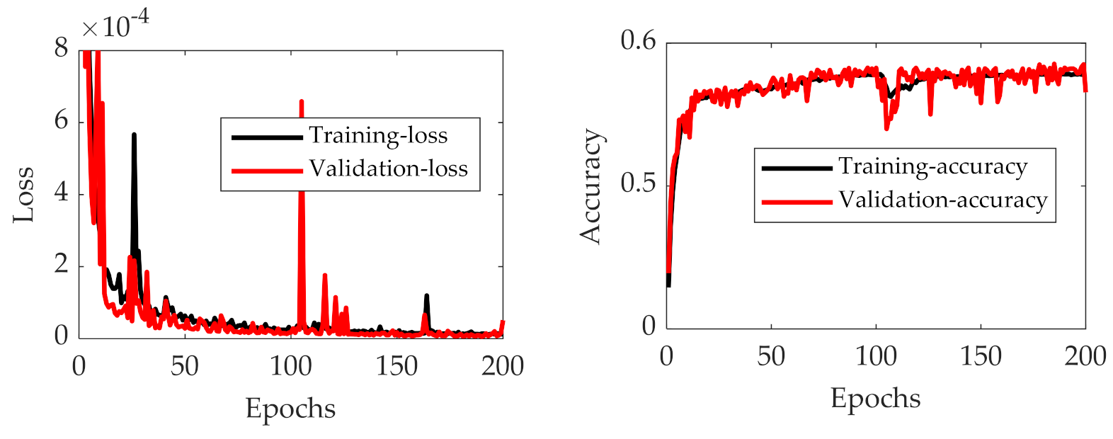
3.4.2. Training and Validation of LSTM-AE Network

To verify the proposed scheme, five case studies were conducted. The aim of these studies was to evaluate different aspects of performance in both steady-state and transient conditions. The case studies verified several aspects of performance of the proposed method including: (1) the performance of the proposed method for estimating grid impedance magnitudes variations at fundamental frequency (50 Hz) due to load changing; (2) the performance of entire proposed scheme when input data sequences included both local and remote locations; (3) the effect of using extracted features instead of using original data sequences; (4) the impact of adding measure data sequence from additional remote nodes to the performance of the proposed scheme; (5) performance comparison of the proposed scheme with the PRBS signal injection method [4] in terms of accuracy, frequency resolution and speed. In all case studies, the performance evaluation criterion for the proposed scheme was the mean square error (MSE) measure as:
M S E i = 1 N i = 1 N z i z ^ i 2
where z i and z ^ i are the i th ground-truth and predicted grid impedance values, respectively, and N is total number of values.
(1) 
Case study 1: performance of the proposed scheme
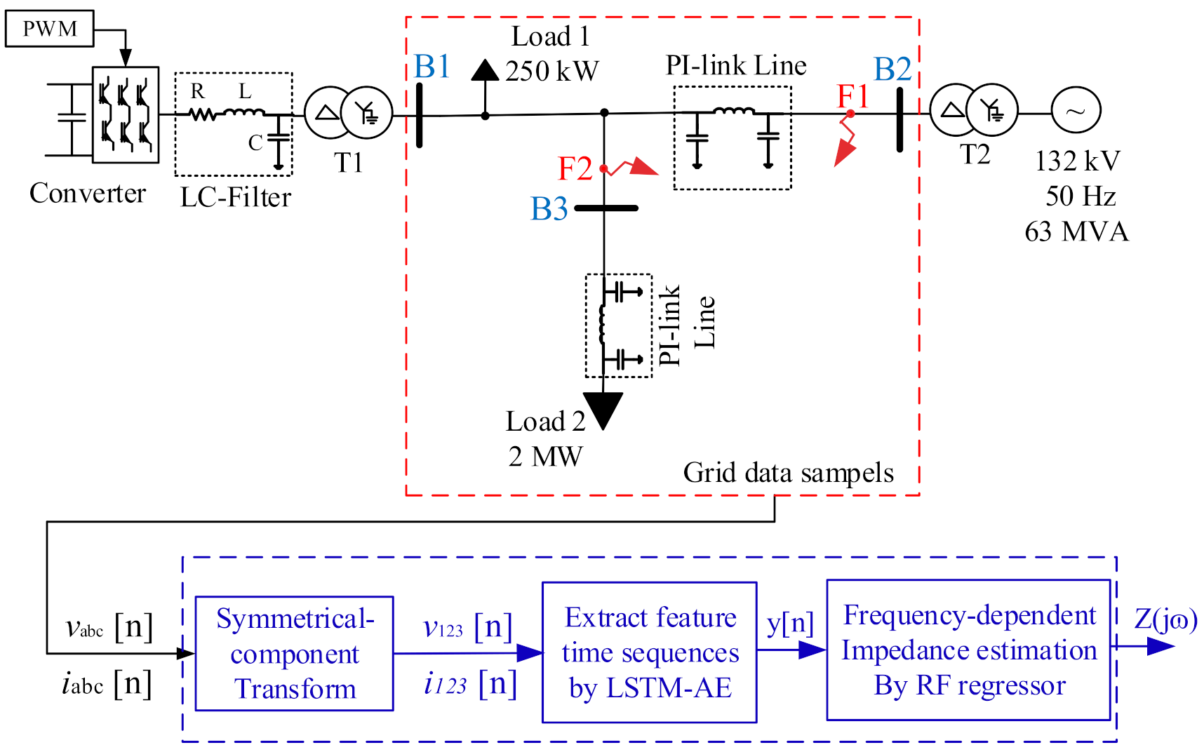
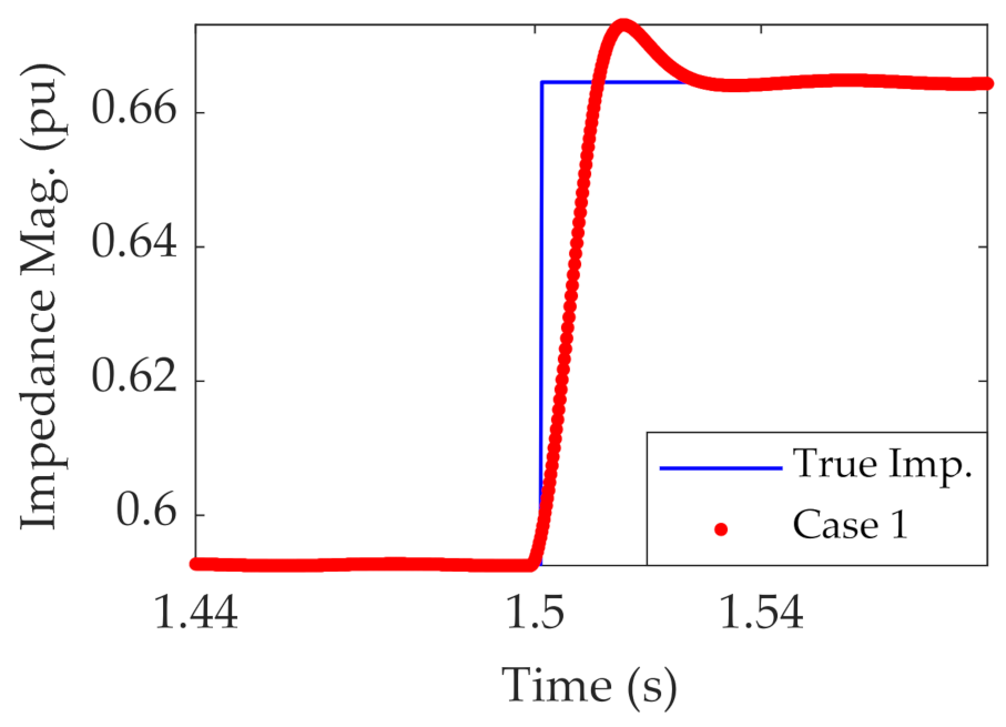
The first case study aimed at verifying the performance of proposed method for estimating the grid impedance magnitude, at fundamental frequency, due to load changing in steady-state condition. The three-phase load, namely Load 1, was changed for 20% pu at time t = 1.5 s. The load change occurred in the power grid steady-state condition. The measurement data are time-series voltage/current data from both the local and remote measurement nodes. The extracted feature vector from the LSTM-AE module was fed into the RF module to estimate the magnitude and phase of the grid impedance over time.
The corresponding MSE of the estimated impedance magnitude is 1.4. Figure 5 shows the result of the grid impedance magnitude estimation at fundamental frequency of the proposed method. The proposed method converged to the grid impedance after 30 ms.
(2) 
Case study 2: performance of the proposed scheme
The second case study aimed at testing the performance of the entire scheme, where measurement data sequences from both the local and remote measurement nodes were used. After the LSTM-AE extracted the feature vector sequences and fed them into the RF, the estimates of the corresponding frequency-dependent grid impedances were obtained. Table 5 shows the results of the proposed scheme in terms of MSE measure.
Observing the third row in Table 5, MSEs of estimated impedances were 1.3 and 3.2. For each fault location (F1 or F2) we used all corresponding 200 datapoints for testing, and the shown MSE in Table 5 is the average of 200 obtained individual MSEs corresponding to each datapoint. 
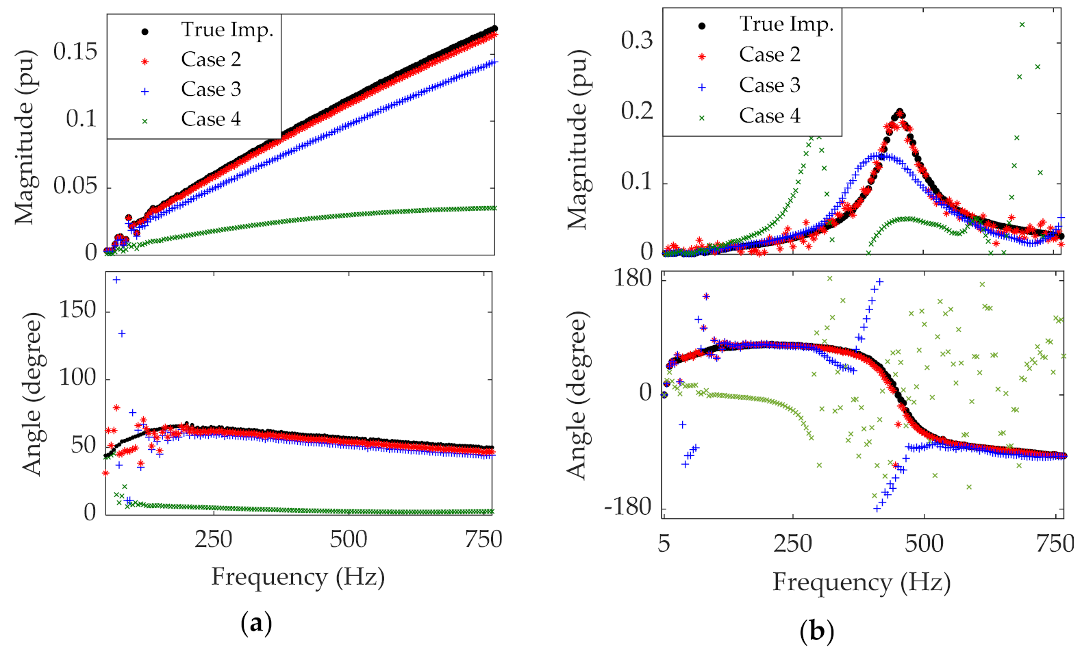
Figure 6a,b (red traces) show the results of grid impedances estimated from the proposed scheme for two random datapoints corresponding to fault locations at F1 and F2.
From the results shown in Figure 5, it can be concluded that the proposed scheme can estimate the grid impedances throughout the set of the selected frequency range. It is worth mentioning that only the positive-sequence frequency-dependent grid impedance is shown in the figure, since the negative-sequence component presented almost identical behavior.
Further, the time required for the proposed scheme is listed in Table 6, split according to different modules.
Observing Table 6, one can see that the training of the LSTM-AE and RF took the most time (180 + 30 min), although training was usually performed once offline. In contrast, the testing process was fast, only requiring a total of 30 ms (1.5 grid cycle) for the combined feature extraction and grid impedance estimation.
(3) 
Case study 3: performance using extracted features
The third case study aimed at verifying the effectiveness of using extracted features instead of raw measurement data for RF regression. In the tests, RF regressor estimated the frequency-dependent grid impedances, whereas the raw data (symmetrical components) was taken instead of extracted features as input. The resulting MSE values are shown in Table 5. Observing Table 5, one can see that without applying feature extraction (i.e., LSTM-AE module) in the proposed scheme, the MSEs of the estimated impedances were 8.4 and 8.67 at points F1 and F2, respectively. The MSE values increased by 7.1 and 5.57 as compared with the first case study where the LSTM-AE module was used. This demonstrates that feature extraction using the LSTM-AE is effective.
To further compare the performance, Figure 6a,b, (blue traces) show the estimated grid impedances at the same data points as those in case study 1. Observing Figure 5, the proposed scheme without employing the LSTM-AE module does not yield a relatively accurate estimation of the grid impedance. The estimation result is very close to the average of all trained datapoints. It can be considered as a drawback of RF for estimating the regression function between time series. As shown in the first case study, extracting sequences of time-dependent features of time series helps the RF regression method to determine the time-dependent relations between input/output data.
(4) 
Case study 4: performance using only local data
The fourth case study aimed at examining the performance impact of the proposed scheme by ignoring an additional measurement data sequence from remote locations. In this study, only the local measurements at node B1 in Figure 1 were used as an input to the LSTM-AE architecture. The fifth row of Table 5 shows the resulting MSE values of the estimated impedances. Observing the results, the MSEs were 20.2 and 46.8 when the electrical faults occurred in points F1 and F2, respectively. The results showed that ignoring remotely measured data leads to a dramatic change in the results.
To further compare the performance, Figure 6 (green traces) shows the estimated frequency-dependent grid impedances seen from node B1 at two random data points, the same as in all previous case studies. Observing the results in Figure 5, one can see that the proposed scheme cannot predict the frequency-dependent grid impedance precisely if the remote measurement data are not used. During fault occurrence the grid structure changes, adding the measurement at remote location and enabling the proposed method to learn the grid structure.
(5) 
Case study 5: comparison with wide-band signal injection method
In the fifth case study, the performance of the proposed scheme was compared with the wide-band PRBS signal injection method [4] in terms of accuracy, frequency resolution and speed.
In the existing method, the PRBS used as the excitation signal was generated by using f x = x 15 + x + 1 , where a sequence was generated under 10 kHz sampling frequency [24]. The PRBS magnitude was set to 1% pu to avoid interfering with the transformer’s no-load voltage tap-changer setting that was approximately 0.5–1.7% on the LV side [25]. The generated PRBS signal was then added to the d -axis reference voltage ( V d ) of the power converter controller. After that, the three-phase voltage and the currents were measured at the node B1 for a duration of 1.0 s. The DFT of the positive-sequence components of both voltage and current were derived to estimate the positive-sequence frequency-dependent grid impedance. The time-domain signal was multiplied by the flat-top window [26] to obtain an approximate periodic signal. It is worth noting that it was not feasible to use the signal injection method for grid impedance estimation during a fault occurrence. Therefore, we compared the PRBS injection and the proposed scheme in the steady-state condition. 
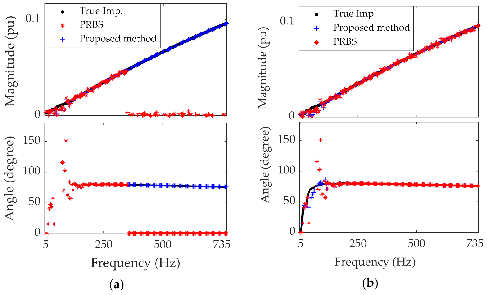
Figure 7a shows the resulting grid frequency estimates using the PRBS signal. Observing the results, the PRBS signal injection method seems to have generated good performance at frequencies below the filter’s cut-off frequency, which is 335 Hz. This case study was then repeated by increasing the PRBS magnitudes to 0.1 pu, and the voltage signals between the RL and RC networks of the filter were measured, as in [4]. Figure 7b shows the obtained result, where the corresponding MSE was 1.4.
The signal injection method was not feasible during large transients. In addition, using a large magnitude for excitation signal might be harmful to other sensitive devices, and the excitation signal with a small magnitude could not be used for estimating the impedance at higher frequencies. Further, the signal injection was slower than the proposed scheme. To estimate grid impedance at lower frequencies like 5 Hz, one needs at least a one-second measurement to perform an acceptable DFT spectrum, while the proposed method needs only one grid cycle measurement value, and the computation demand is 30 ms.

3.5. Discussion

From the test results, the following important observations were obtained:
  • LSTM-AE model for automatic feature extraction: The results show that the LSTM-AE is an effective method for extracting sequential features of time series and consequently improves the RF regression estimation for time-series data.
  • Data from remote locations: The results in case study 3 showed that adding measurements at remote nodes ensures the estimation during large disturbances even the RF model is trained on steady-state data. However, the main challenges for remote measurement are: (1) the latency due to data communication from remote nodes to the local area; (2) considering the related cost, it is not possible to conduct measurement at all nodes of the power grid; (3) the number and the location of best nodes for remote measuring are unknown.
  • Time-delay in measurement data: The time-delay in measurement data was ignored in this study, assuming that the measurement was conducted under 5G internet protocols, which introduce the ultra-reliable low-latency communication (URLLC) system that guarantees reliability of 99.999% and latency of less than 1 ms [27].
Future works will further verify the proposed method through real measured power grid data for different utility grids by considering several grid-connected power converters as well as a qualitative and quantitative search for the best location and best number of remote location measurements.

4. Conclusions

This paper proposes a deep-learning-based method for estimating frequency-dependent grid impedance. The method consists of an unsupervised sequential feature learning module employing the LSTM autoencoder (LSTM-AE) model, followed by a random forest (RF) regressor module for impedance estimation. The proposed method was trained on a large synthetic dataset (2000 measurement sets, i.e., one grid cycle (200 samples) of 18 symmetrical components of voltage/current data) generated when the power system was in steady-state condition.
The results showed that extracting the time-dependent features of power grid time series improved the RF regressor performance. Further, the results showed that the effectiveness of the RF regressor during large transients is highly dependent on remote location measurement data.
The proposed method was compared with the state-of-the-art PRBS signal injection method. The proposed method can estimate the grid impedance at both steady-state and transient condition, while the PRBS method is only feasible at steady-state condition. The time required for proposed method to extract sequential features of one grid cycle data sample and then predict the corresponding grid impedance is 30 ms, whereas the time required for the PRBS method to estimate the same grid impedance is longer than 1 s.

Author Contributions

Investigation, review and editing, A.B.; writing and editing, A.B.; editing and project administration, M.B., I.Y.H.G. and J.R.S. All authors have read and agreed to the published version of the manuscript.

Funding

The financial support provided by Energimyndigheten through the SamspEL program is gratefully acknowledged.

Institutional Review Board Statement

Not applicable.

Informed Consent Statement

Not applicable.

Data Availability Statement

Not applicable.

Conflicts of Interest

The authors declare no conflict of interest.

Abbreviations

DFTDiscrete Fourier transform
LSTM-AELong short-term memory autoencoder
MSEMean square error
PRBSPseudorandom binary signal
RFRandom forest
ReLURectified linear unit
RNNRecursive neural network
SVMSupport vector machine
URLLCUltra-reliable low-latency communication

References

  1. Harnefors, L.; Bongiorno, M.; Lundberg, S. Input-admittance calculation and shaping for controlled voltage-source converters. IEEE Trans. Ind. Electron. 2007, 54, 3323–3334. [Google Scholar] [CrossRef]
  2. Xu, J.; Xie, S.; Qian, Q.; Zhang, B. Adaptive feedforward algorithm without grid impedance estimation for inverters to suppress grid current instabilities and harmonics due to grid impedance and grid voltage distortion. IEEE Trans. Ind. Electron. 2017, 64, 7574–7586. [Google Scholar] [CrossRef]
  3. Cobreces, S.; Bueno, E.J.; Pizarro, D.; Rodriguez, F.J.; Huerta, F. Grid impedance monitoring system for distributed power generation electronic interfaces. IEEE Trans. Instrum. Meas. 2009, 58, 3112–3121. [Google Scholar] [CrossRef]
  4. Roinila, T.; Vilkko, M.; Sun, J. Broadband methods for online grid impedance measurement. In Proceedings of the 2013 IEEE Energy Conversion Congress and Exposition, Denver, CO, USA, 15–19 September 2013; pp. 3003–3010. [Google Scholar]
  5. Sanchez, S.; Molinas, M. Large signal stability analysis at the common coupling point of a DC microgrid: A grid impedance estimation approach based on a recursive method. IEEE Trans. Energy Convers. 2014, 30, 122–131. [Google Scholar] [CrossRef]
  6. Hoffmann, N.; Fuchs, F.W. Minimal invasive equivalent grid impedance estimation in inductive–resistive power networks using extended Kalman filter. IEEE Trans. Power Electron. 2013, 29, 631–641. [Google Scholar] [CrossRef]
  7. Alves, D.K.; Ribeiro, R.L.; Costa, F.B.; Rocha TO, A. Real-time wavelet-based grid impedance estimation method. IEEE Trans. Ind. Electron. 2018, 66, 8263–8265. [Google Scholar] [CrossRef]
  8. Asiminoaei, L.; Teodorescu, R.; Blaabjerg, F.; Borup, U. Implementation and test of an online embedded grid impedance estimation technique for PV inverters. IEEE Trans. Ind. Electron. 2005, 52, 1136–1144. [Google Scholar] [CrossRef]
  9. Ghanem, A.; Rashed, M.; Sumner, M.; Elsayes, M.A.; Mansy, I.I. Grid impedance estimation for islanding detection and adaptive control of converters. IET Power Electron. 2017, 10, 1279–1288. [Google Scholar] [CrossRef]
  10. Asiminoaei, L.; Teodorescu, R.; Blaabjerg, F.; Borup, U. A digital controlled PV-inverter with grid impedance estimation for ENS detection. IEEE Trans. Power Electron. 2005, 20, 1480–1490. [Google Scholar] [CrossRef]
  11. Liserre, M.; Blaabjerg, F.; Teodorescu, R. Grid impedance estimation via excitation of LCL -filter resonance. IEEE Trans. Ind. Appl. 2007, 43, 1401–1407. [Google Scholar] [CrossRef]
  12. Givaki, K.; Seyedzadeh, S. Machine learning based impedance estimation in power system. In Proceedings of the 8th Renewable Power Generation Conference (RPG 2019), Shanghai, China, 24–25 October 2019. [Google Scholar]
  13. Céspedes, M.; Sun, J. Online grid impedance identification for adaptive control of grid-connected inverters. In Proceedings of the 2012 IEEE Energy Conversion Congress and Exposition (ECCE), Raleigh, NC, USA, 15–20 September 2012; pp. 914–921. [Google Scholar]
  14. Mohammed, N.; Ciobotaru, M.; Town, G. Online parametric estimation of grid impedance under unbalanced grid conditions. Energies 2019, 12, 4752. [Google Scholar] [CrossRef] [Green Version]
  15. Gensler, A.; Henze, J.; Sick, B.; Raabe, N. Deep Learning for solar power forecasting—An approach using AutoEncoder and LSTM Neural Networks. In Proceedings of the 2016 IEEE International Conference on Systems, Man, and Cybernetics (SMC), Budapest, Hungary, 9–12 October 2016; pp. 002858–002865. [Google Scholar]
  16. Policardi, F. MLS and Sine-Sweep measurements. Università di Bologna. Ital. Elektroteh. Vestn. 2011, 78, 91–95. [Google Scholar]
  17. Srivastava, N.; Mansimov, E.; Salakhudinov, R. Unsupervised learning of video representations using lstms. In Proceedings of the International Conference on Machine Learning, Lille, France, 6–11 July 2015; pp. 843–852. [Google Scholar]
  18. Sagheer, A.; Kotb, M. Unsupervised pre-training of a deep LSTM-based stacked autoencoder for multivariate time series forecasting problems. Sci. Rep. 2019, 9, 1–16. [Google Scholar] [CrossRef] [Green Version]
  19. Ge, C.; de Oliveira, R.A.; Gu IY, H.; Bollen, M.H. Deep Feature Clustering for Seeking Patterns in Daily Harmonic Variations. IEEE Trans. Instrum. Meas. 2020, 70, 1–10. [Google Scholar] [CrossRef]
  20. Statnikov, A.; Wang, L.; Aliferis, C.F. A comprehensive comparison of random forests and support vector machines for microarray-based cancer classification. BMC Bioinform. 2008, 9, 1–10. [Google Scholar] [CrossRef] [Green Version]
  21. Breiman, L. Random forests. Mach. Learn. 2001, 45, 5–32. [Google Scholar] [CrossRef] [Green Version]
  22. Liaw, A.; Wiener, M. Classification and regression by random Forest. R News 2002, 2, 18–22. [Google Scholar]
  23. Nowozin, S. Improved information gain estimates for decision tree induction. arXiv 2012, arXiv:1206.4620v1. [Google Scholar]
  24. Bagheri, A.; Gu, I.Y.; Bollen, M.H.; Balouji, E. A robust transform-domain deep convolutional network for voltage dip classification. IEEE Trans. Power Deliv. 2018, 33, 2794–2802. [Google Scholar] [CrossRef]
  25. Barker, H.A. Primitive maximum-length sequences and pseudo-random signals. Trans. Inst. Meas. Control. 2004, 26, 339–348. [Google Scholar] [CrossRef]
  26. Gajić, Z.; Aganović, S. Advanced Tapchanger Control to Counteract Power System Voltage Instability 2006. Available online: https://library.e.abb.com/public/9acc3c82f0230659c125766900481ca1/1MRG001019_en_Advanced_Tapchanger_Control_To_Counteract_Power_System_Voltage_Instability.pdf (accessed on 22 May 2021).
  27. Sachs, J.; Wikstrom, G.; Dudda, T.; Baldemair, R.; Kittichokechai, K. 5G radio network design for ultra-reliable low-latency communication. IEEE Netw. 2018, 32, 24–31. [Google Scholar] [CrossRef]
Figure 1. The overall schematic of the proposed method: power grid (red dashed line box), the deep-learning-based nonlinear estimator (blue dashed line box).
Energies 14 03829 g001
Figure 2. The proposed LSTM autoencoder; (a) the overall architecture of LSTM-AE (input layer + 1 LSTM-AE layer); (b) 10 concatenated sequences of time-dependent features extracted for 1 cycle data; (c) the LSTM-AE architecture during the training process.
Energies 14 03829 g002
Figure 3. Decision trees of RF regressor, obtained from the training process of the proposed scheme.
Energies 14 03829 g003
Figure 4. Performance from the training and validation in the proposed LSTM-AE; (left) loss versus epochs, (right) accuracy versus epochs.
Energies 14 03829 g004
Figure 5. The result of estimating the fundamental (50 Hz) grid impedance magnitude at node B1, due to step change in Load 1, compared with true impedance (True Imp.).
Energies 14 03829 g005
Figure 6. The result of estimating the frequency-dependent grid impedance at node B1 compared with true impedance (True Imp.) obtained by sine sweep; (a) three-phase fault is located at F1, impedance magnitudes (top), phase angles (bottom); (b) three-phase fault located at F2, impedance magnitudes (top), phase angles (bottom).
Energies 14 03829 g006
Figure 7. Case study 5: The result of estimating the frequency-dependent grid impedance magnitude (top) and angle (bottom) at node B1, at steady-state condition, using the proposed method and PRBS injection method; (b) voltage signals were measured at node B1, and the PRBS magnitude was 0.01 pu, (a) voltage signals were measured at the point between the filter’s RL and RC networks, and the PRBS magnitude was 0.1 pu.
Energies 14 03829 g007
Table 1. Architecture of the encoder of the proposed LSTM-AE.
LayersNumber of CellsNumber of Units/CellUnit InputUnit Output
Input layer [20 × 18] - -
LSTM-AE 1 + ReLU201620 × 1820 × 16
LSTM-AE 2 + ReLU20820 × 161 × 8
Table 2. The detailed parameters of the simulated power network.
DescriptionValues
Overhead   line   ( positive   seq . ) ,   l 1 , c 1 ,   r 1 1.05   mH , 0.33   μ F , 0.1153 Ω
Overhead   line   ( zero   seq . ) ,   l 0 , c 0 ,   r 0 3.32   mH , 5.01   nF , 0.413 Ω
Load 1: voltage, P33 kV, 250 kW
Load 2: voltage, P33 kV, 2 MW
Converter :   DC   link   voltage ,   f p w m , S600 V, 1980 Hz, 250 kVA
Transformer 1: V1/V2, S415 V/33 kV, 250 kVA
Transformer 2: V1/V2, S132/33 kV, 63 MVA
Table 3. The size of training/test datasets for both LSTM-AE and RF regression models.
DatasetSizeModels
LSTM-AERF
Training (Dataset 1)Input size[1200, [10, 20], 18][1200, 80]
Output size[1200, [10, 20], 18][1200, 306]
Validation (Dataset 1)Input size[800, [10, 20], 18][800, 80]
Output size[800, [10, 20], 18][800, 306]
Testing (Dataset 2)Input size[600, [10, 20], 18][600, 80]
Output size[600, [10, 20], 18][600, 306]
Table 4. Finding the best RF structure that minimizes MSE values through grid search.
Depth of Trees
Number of Decision Trees102550
2520.08.327.13
505.463.204.86
759.148.419.69
1005.376.368.80
Table 5. The overall performance of proposed method in terms of mean square error (MSE) over total test dataset.
Mean Square Error
Fault locationF1F2
Case study 11.33.2
Case study 28.48.67
Case study 320.246.8
Table 6. Time required for training different modules of the proposed method, feature extraction and impedance estimation.
ProcessTaskTime (s)
TrainingLSTM-AE10,800 (or 180 min)
TrainingRF regressor1800 (or 30 min)
TestingFeature extraction for one datapoint0.02
TestingGrid impedance estimation for one datapoint0.01
Publisher’s Note: MDPI stays neutral with regard to jurisdictional claims in published maps and institutional affiliations.

