Performance of Supercritical CO₂ Power Cycle and Its Turbomachinery with the Printed Circuit Heat Exchanger with Straight and Zigzag Channels

Abstract

Since printed circuit heat exchangers (PCHE) are the largest modules of a supercritical carbon dioxide Brayton cycle, they can considerably affect the whole system’s performance and layout. Straight-channel and zigzag-channel printed circuit heat exchangers have frequently been analyzed in the standalone mode and repeatedly proposed for $sC{O}_2-BC$. However, the impact of heat exchanger designs with straight and zigzag-channel configurations on the performance of the cycle and its components, i.e., the turbine and compressor, has not been studied. In this context, this study evaluates the effect of different heat exchanger designs with various values of effectiveness ($ϵ$), inlet Reynolds number (Re), and channel configuration (zigzag and straight channel) on the overall performance of the $sC{O}_2-BC$ and its components. For the design and analysis of PCHEs, an in-house PCHE design and analysis code (PCHE-DAC) was developed in the MATLAB environment. The $sC{O}_2-BC$ performance was evaluated utilizing an in-house cycle simulation and analysis code (CSAC) that employs the heat exchanger design code as a subroutine. The results suggest that pressure drop in PCHEs with straight-channel configuration is up to 3.0 times larger than in PCHEs with zigzag-channel configuration. It was found that a higher pressure drop in the PCHEs with straight channels can be attributed to substantially longer channel lengths required for these designs (up to 4.1 times than zigzag-channels) based on the poor heat transfer characteristics associated with these channel geometries. Thus, cycle layouts using PCHEs with a straight-channel configuration impart a much higher load (up to 1.13 times) on the recompression compressor, this in turn, results in a lower pressure ratio across the turbine. Therefore, the overall performance of the $sC{O}_2-BC$ using PCHEs with straight-channel configurations is found to be substantially inferior to that of layouts using PCHEs with zigzag-channel configurations. Finally, optimization results suggest that heat exchanger’s design with inlet Reynolds number and heat exchanger effectiveness ranging from $32 \mathrm{k}$ to $42 \mathrm{k}$ and $0.94>ϵ>0.87$, respectively, are optimal for $sC{O}_2-BC$ and present a good bargain between cycle efficiency and its layout size.

1. Introduction

Supercritical power systems have recently gained widespread attention because they offer advantages in multiple industry sectors. Primarily, it is expected that they can significantly improve energy conversion efficiency, create new markets because of their smaller size combined with higher efficiency, and are economically more viable. The potential applications for $sC{O}_2$-Brayton cycle in particular, are extensive because it can be used in any application that uses a Rankine cycle, including power generation. Major competitors of the $sC{O}_2-BC$ that have been well studied are Rankine and Air Brayton cycles. One of the chief advantages linked with the Rankine power cycle is its high work ratio against small pumping power requirements. In contrast, the Air Brayton cycle can operate at excessively high turbine inlet temperatures. However, the former’s operation is limited by high turbine inlet temperature, and high compression power requirements are linked with the latter. These disadvantages can be tackled by the novel $sC{O}_2-BC$. The main-compressor of the novel $sC{O}_2-BC$ operates near the critical point of its working fluid. Its compressibility factor is comparable to liquids (0.2–0.5) [1] and as a result, compression work for the cycle is minimal. Furthermore, it can gain high thermal efficiency due to its capability to operate at very high turbine inlet temperatures. Apart from its ability to achieve higher thermal efficiency, the cycle layout of the $sC{O}_2-BC$ is compact and straightforward [1,2] (at least ten times more compact in Comparison with the Rankine Cycle) due to its operation at very high pressure (7.3–30 MPa).This makes it an ideal cycle for power generation [1,2,3].

Numerous combinations of $sC{O}_2-BC$ have been analyzed to enhance its performance [4,5,6,7,8] further. The basic $sC{O}_2-BC$, well-known as a simple recuperating or regenerative cycle involves a regenerator, a primary heat exchanger/heater, a pre-cooler, a compressor, and a turbine. It was first suggested by Feher [9]. Other arrangements of the recuperation/regenerative cycle include reheated-compression and intercooled-recompression [4,5,6,7]. Recompression $sC{O}_2-BC$ with an extra recuperator has been referred to as one of the most efficient arrangements of the $sC{O}_2$ Brayton cycle by many researchers [7,8,10,11,12]. Several studies have been performed with an emphasis on augmenting the $sC{O}_2-BC$ recompressor. Sarkar and Bhattacharyya [13] conducted a study to optimize the $sC{O}_2-BC$ with a reheater. They evaluated the effect of different cycle parameters, including cycle pressure ratio $\left(Pr\right)$, operating temperature/pressure effectiveness of the high-temperature recuperator (HTR), and effectiveness of the low-temperature recuperator (LTR). They reported a maximum turbine temperature of 750 °C; recompression cycles with and without a reheater exhibited cycle efficiencies of 50.78% and 49.83%, respectively. Reyes-Belmonte et al. [7] conducted an optimization study for an $sC{O}_2-BC$ for application in central receiver solar power plants. Optimization of an $sC{O}_2-BC$ for application in a marine gas turbine was conducted by Sharma et al. [14]. Pressure drop effectiveness and recuperator effectiveness on the performance of $sC{O}_2-BC$ were investigated by Sarkar et al. [15] based on the 2nd law efficiency.

The enhanced theoretical performance attracted researchers in academics and industry. In a review paper, Crespi et al. [16] reported 42 standalone and 38 combined cycle layouts that were proved to be theoretically competitive. In 2009, Sandia National Laboratory [17] in the US built a $250 k{W}_e$ recompression cycle experimental loop. In 2014, the US Department of Energy designed the Supercritical Transformational Electric Power crosscut initiative with nuclear and fossil fuels [18]. Saeed et al. [2,19] evaluated the performance of the $sC{O}_2-BC$ using detailed models of each component. Li et al. [20] performed a comparative study on the vapor absorption cycle integrated with the $sC{O}_2-BC$. Wang and He [21] performed an optimization study for $sC{O}_2-BC$ using molten salt solar power as a heat source. Wang et al. [22] performed investigations for two-stage recompression Brayton cycle linked with the high-temperature energy storage system. Several studies [23,24,25] have been conducted in the literature on the integration of the $sC{O}_2-BC$ with Organic Rankine Cycle (ORC). Concerning the application of the cycle to different existing energy conversion systems, Kim et al. [26] analyzed the potential of supercritical $C{O}_2$ Rankine cycle for the waste heat recovery while, Luu et al. [27] investigated supercritical $C{O}_2$ Brayton cycle for its integration with the concentrated solar power plants (CSP).

It can be inferred from the literature survey that although several studies have been conducted to analyze the $sC{O}_2-BC$ no study has been conducted to evaluate the impact of different PCHE designs on the cycle and its turbomachinery. While Saeed et al. [28,29] studied the effects of different PCHE designs on the performance of $sC{O}_2-BC$; no study has reported the influence of different PCHE designs on the performance of the cycle’s components, i.e., turbines and compressors. In this perspective, the current research evaluates the impact of zigzag and straight-channel PCHEs on the cycle’s performance and its components. In this study, an in-house PCHE design and analysis code (PCHE-DAC) was used for the PCHE design and analysis to compute the effect of Reynolds number $\left(Re\right)$, effectiveness $\left(ϵ\right)$ and channel configurations (straight and zigzag) on the initial PCHE size and performance. Heat exchanger designs with straight and zigzag-channel geometries and other parameters, i.e., $ϵ,$ and $Re$ are used to investigate the effects on the turbomachinery design and overall cycle performance. An in-house Cycle simulation and analysis code (DDPC) was used to compute the cycle performance at its design point. Properties of sCO₂ have been incorporated in the code by coupling with NIST REFPROP. An optimized design based on the straight and zigzag channels has been proposed for the $sC{O}_2-BC$. Because the performance, size, and layout of the $sC{O}_2-BC$ power cycle are extremely sensitive to the design and performance of its PCHEs; current study provides valuable data and guidelines to further enhance the performance and layout of the $sC{O}_2-BC$.

2. Numerical Models and Methodology

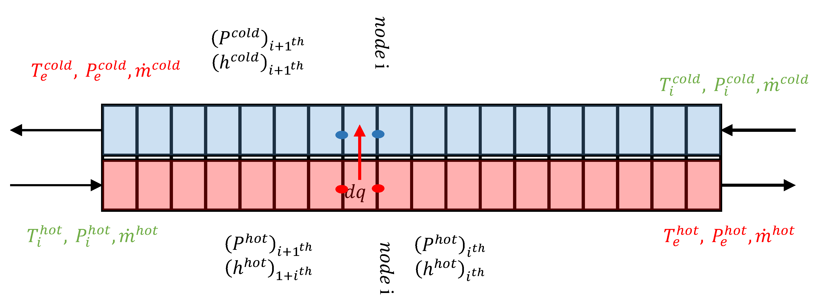
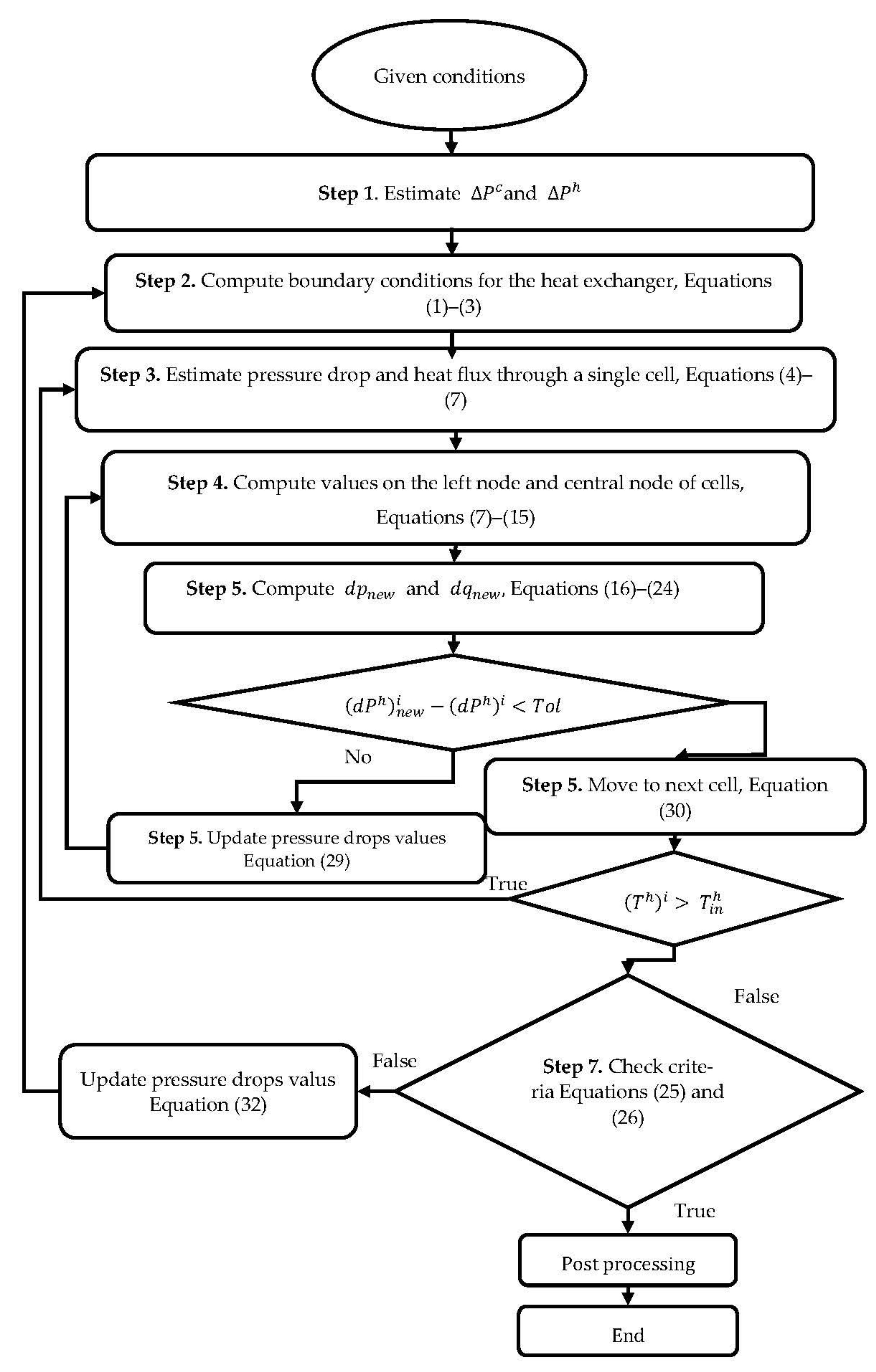
2.1. Mathematical Model for PCHE Design and Analysis Code (PCHE-DAC)

The mathematical model adopted for PCHE-DAC in the current study is based on a discretized LMTD method used and developed by Saeed et al. [2,30,31]. A heat exchanger code was built based on this model; pressure drop and heat transfer correlation used for the current study are listed in

Table 1. Pressure drop and heat transfer correlations for the PCHEs.

Configuration	Correlations	Channel Geometry
Genelisi [32]	$Nu =\frac{ \left(f/8\right)\left(Re-1000\right)Pr}{1+12.7{\left(\frac{f}{8}\right)}^{0.5}*\left({\mathrm{Pr}}^{\frac{2}{3}}-1\right)}$ $f ={\left(\frac{1}{1.8log10\left(Re\right)-1.5}\right)}^2$ $\left(3,000\le Re\le 60,000\right)$ $\left(0.7\le Pr\le 1.2\right)$
Ishizuka et al. [33]	$h=0.210Re+44.16$ $f=-2\times {10}^{-6}Re+0.1023$ $\left(5,000\le \mathrm{Re}\le 13,000\right)$ $\left(\mathsf{\theta }={40}^0\right)$
Kim et al. [34]	$Nu =0.0292R{e}^{0.8742}$$, f =0.2515R{e}^{-0.2031}$$; (\mathsf{\theta }= {32}^0$) $Nu =0.0188R{e}^{0.8742}$$, f =0.2881R{e}^{-0.1322}$$; (\mathsf{\theta }= {40}^0)$ $\left(2,000\le Re\le 58,000\right)$ $\left(0.7\le Pr\le 1.0\right)$
Saeed and Kim [35]	$Nu =0.041R{e}^{0.83}P{r}^{0.95}$$, f =0.115R{e}^{-0.13}$$;(\mathsf{\theta }= {40}^0$) $\left(3,000\le Re\le 60,000\right), \left(0.7\le Pr\le 1.2\right)$

. The number of divisions (n) used to discretize the model (Figure 1) was ensured to be sufficient to capture the steep variations in the thermophysical properties of the working fluid ($sC{O}_2$). The following procedure has been adopted to study the printed circuit heat exchanger.

It is assumed that the header of the heat exchanger distributes the flow to all channels uniformly. Heat losses to the surroundings are exceedingly small and can be ignored. It is also assumed that the flow and heat transfer characteristics in a unit consisting of one channel from the hot and cold side each can represent the behavior of the whole heat exchanger, as shown in Figure 1. The blue and red colors used in Figure 1 demonstrate the heat exchanger’s cold and hot sides, respectively. Hot and cold fluids in their respective channels flow in the counterclockwise direction. The state of working fluids at both hot and cold side inlets is known (marked green), while the exit condition (characterized as red) is unknown. It should be noted here that the formulation is given in the section below, and Figure 2 is provided for the $i^{th}$ segment bounded by the side node, i.e., $i^{th}$ and $i+1^{th}$ node.

Step 1. Estimate the values of $\mathsf{\Delta }{P}^{cold}$ and $\mathsf{\Delta }{P}^{hot}$.

Step 2. Using known inlet condition values, exit conditions for both hot and cold channels were computed using the effectiveness value. The working fluid’s thermophysical properties were calculated as a function of temperature and pressure by linking NIST REFPROP with the MATLAB code via a subroutine. The procedure for calculating the exit condition is given in the following equations.

$$ϵ=\frac{h_i^{hot}-h_e^{hot}}{h_i^{hot}-h\left(P_o^{hot}, T_i^{hot}\right)}=\frac{h_e^{cold}-h_i^{cold}}{h_i^{hot}-h\left(P_e^{hot}, T_i^{hot}\right)}$$

(1)

$$\left(h_e^{cold}-h_i^{cold}\right)= \left(h_i^{hot}-h_o^{cold}\right)$$

(2)

$$P_o^{cold}=P_i^{cold}- \mathsf{\Delta }{P}^{cold}$$

(3)

Step 3. Current conditions at the inlet and outlet of the heat exchanger can be used to compute the initial pressure drop and heat transfer values through each cell, as demonstrated in the following equations.

$${\left(d{P}^{cold}\right)}_{i^{th}}=\mathsf{\Delta }{P}^{cold}/n$$

(4)

$${\left(d{P}^{hot}\right)}_{i^{th}}= \mathsf{\Delta }{P}^{hot}/n$$

(5)

$${\left(d{q}^{cold}\right)}_{i^{th}}=(h_i^{cold}-h_e^{cold})/$$

(6)

$${\left(d{q}^{hot}\right)}_{i^{th}}={\left(d{q}^{cold}\right)}_{i^{th}}$$

(7)

Step 4. Once quantities in the $i^{th}$ cell are known, the ${\left(i+1\right)}^{th}$ cell can be computed using the following equation. Further mean values at the cell center were computed by taking an average of the $i^{th}$ and ${\left(i+1\right)}^{th}$ values.

$${\left(h^{cold}\right)}_{i+1^{th}}={\left(h^{cold}\right)}_{i^{th}}+\frac{{\left(d{q}^{cold}\right)}_{i^{th}}}{m^{cold}}$$

(8)

$${\left(P^{cold}\right)}_{i+1^{th}}={\left(P\right)}_{i^{th}}-{\left(d{p}^{cold}\right)}_{i^{th}}$$

(9)

$${\left(h^{hot}\right)}_{i+1^{th}}={\left(h^{hot}\right)}_{i^{th}}-\frac{{\left(d{q}^{cold}\right)}_{i^{th}}}{m^{hot}}$$

(10)

$${\left(P^{hot}\right)}_{i+1^{th}}={\left(P\right)}_{i^{th}}+{\left(d{p}^{hot}\right)}_{i^{th}}$$

(11)

$${\left(h_{mean}^{cold}\right)}_{i+1^{th}}={\left(h^{cold}\right)}_{i^{th}}+0.5\frac{{\left(d{q}^{cold}\right)}_{i^{th}}}{m^{cold}}$$

(12)

$${\left(P_{mean}^{cold}\right)}_{i+1^{th}}={\left(P\right)}_{i^{th}}-0.5{\left(d{p}^{cold}\right)}_{i^{th}}$$

(13)

$${\left(h_{mean}^{hot}\right)}_{i+1^{th}}={\left(h^{hot}\right)}_{i^{th}}-0.5\frac{{\left(d{q}^{cold}\right)}_{i^{th}}}{m^{hot}}$$

(14)

$${\left(h_{mean}^{hot}\right)}_{i+1^{th}}={\left(h^{hot}\right)}_{i^{th}}-\frac{{\left(d{q}^{cold}\right)}_{i^{th}}}{m^{hot}}$$

(15)

Step 5. In the next step, the working fluid properties were computed based on the pressure and enthalpy’s cell-centered values to calculate the friction factor and overall heat transfer coefficient, which were used to calculate new pressure drop and heat transfer values as shown in the following equations. It should be noted here that friction factor and heat transfer coefficient value were computed using correlations provided in Table 1.

$${({\rho }_{mean}^{cold},{\mu }_{mean}^{cold},C{p}_{mean}^{cold}, {\mathrm{Pr}}_{mean}^{cold}, T_{mean}^{cold})}_{i^{th}} =f\left(h_{mean}^{cold}, P_{mean}^{cold}\right)$$

(16)

$${\left({\rho }_{mean}^{hot},{\mu }_{mean}^{hot},C{p}_{mean}^{hot}, {\mathrm{Pr}}_{mean}^{hot}, T_{mean}^{hot}\right)}_{i+1^{th}}=f\left(h_{mean}^{hot}, P_{mean}^{hot}\right)$$

(17)

$${\left(f^{cold}\right)}_{i^{th}}=f{\left( R{e}_{mean}^{cold}\right)}_{i^{th}}$$

(18)

$${\left(f^{hot}\right)}_{i^{th}}=f{\left( R{e}_{mean}^{hot}\right)}_{i^{th}}$$

(19)

$${\left(h^{cold}\right)}_{i^{th}}=f{\left( R{e}_{mean}^{cold},P{r}_{mean}^{cold}\right)}_{i^{th}}$$

(20)

$${\left(h^{hot}\right)}_{i^{th}}=f{\left( R{e}_{mean}^{hot},P{r}_{mean}^{hot}\right)}_{i^{th}}$$

(21)

$${\left(UA\right)}_{i^{th}}=\frac{1}{\frac{1}{{\left(h^{cold}\right)}_{i^{th}}}+\frac{k}{t}+\frac{1}{{\left(h^{hot}\right)}_{i^{th}}}}$$

(22)

$${\left(d{p}_{new}^{cold}\right)}_{i^{th}}=\frac{{\left(f^{cold}\right)}_{i^{th}} {\left(m^c\right)}^2 }{2D_{hyd}^c{\left({\rho }^{cold}\right)}_{i^{th}}{A}_x^c{}^2}dx$$

(23)

$$\{\begin{array}{c}i=i+1\\ {\left(d{p}_{new}^{cold}\right)}_{i^{th}}={\left(d{P}^{cold}\right)}_{i^{th}},{\left(d{P}^{cold}\right)}_{i^{th}}= {\left(d{P}^{cold}\right)}_{i-1^{th}}\\ {\left(d{q}_{new}^{cold}\right)}_{i^{th}}={\left(d{q}^{cold}\right)}_{i^{th}},{\left(d{q}^{cold}\right)}_{i^{th}}= {\left(d{q}^{cold}\right)}_{i-1^{th}} \end{array}$$

(24)

Step 6. The next step controls the convergence of the solution of Equation (24) until all cells are computed.

Step 7. The outer loop controls the convergence of boundary conditions, as given in the following equation.

$$\{\begin{array}{c}{\left(h^{hot}\right)}_{n^{th}} -h_{out}^{hot}<Tol\\ {\left(h^{cold}\right)}_{n^{th}} -h_{out}^{cold}<Tol\end{array}$$

(25)

$$\{\begin{array}{c}\mathsf{\Delta }{P}^{hot}={\left(h^{hot}\right)}_{n^{th}}-{\left(h^{hot}\right)}_{1^{st}}\\ \mathsf{\Delta }{P}^{cold}={\left(h^{cold}\right)}_{n^{th}}-{\left(h^{cold}\right)}_{1^{st}}\end{array}$$

(26)

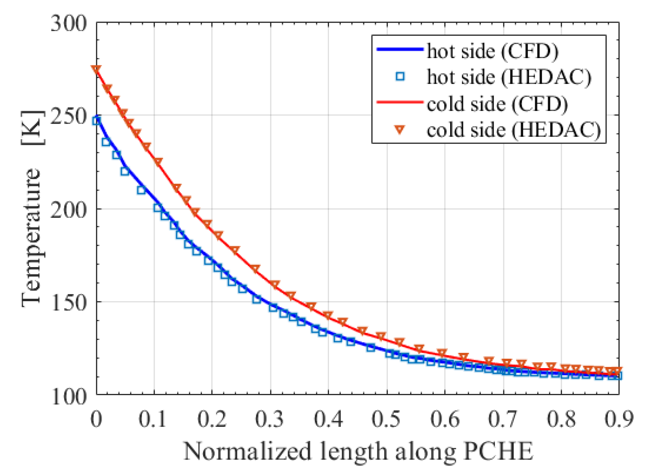
Validation for the PCHE Design and Analysis Code (PCHE-DAC)

PCHE design and analysis code (PCHE-DAC) was validated by utilizing a two-step validation procedure that involves both validations of the conditions at boundaries along with the validation of data at every nodal point along the PCHE’s length. Validation of conditions at boundaries was carried by comparing the code boundary data with the experimental results of Ishizuka et al. [33]. On the other hand, the validation of the nodal data was conducted by comparing the temperature profiles obtained from the code with the temperature profiles extracted from the previous study’s CFD results [3]. Numerical results employed for the validation were taken from the CFD model [3] that was authenticated using experimental data [33]. The validation purpose’s boundary conditions are listed in

Table 2. Details of the boundary conditions used for the validation study.

Hot Side			Cold Side
$P_{in}^h\left[\mathrm{kPa}\right]$	$T_{in}^h\left[oC\right]$	$m^h\left[{\mathrm{kg} \mathrm{s}}^{-1}\right]$	$P_{in}^c\left[\mathrm{kPa}\right]$	$T_{in}^c\left[oC\right]$	$m^c\left[{\mathrm{kg} \mathrm{s}}^{-1}\right]$
2520	279.9	0.0001445	8353.22	107.9	0.0003152

, while a comparison of the PCHE-DAC data with the experimental data is provided in

Table 3. Assessment of the printed circuit heat exchanger design and analysis code PCHE-DAC and experimental data.

	PCHE-DAC	Experimental Results	% Difference
$\mathsf{\Delta }{T}^h\left[oC\right]$	169.20	161.5	4.5%
$\mathsf{\Delta }{T}^c\left[oC\right]$	142.90	141.1	5.18%

. Validation of the computed data suggests the maximum difference between the code and experimental results is around 5%. On the other hand, comparison of the nodal data (Figure 3) indicate that code data is in close agreement with the CFD data.

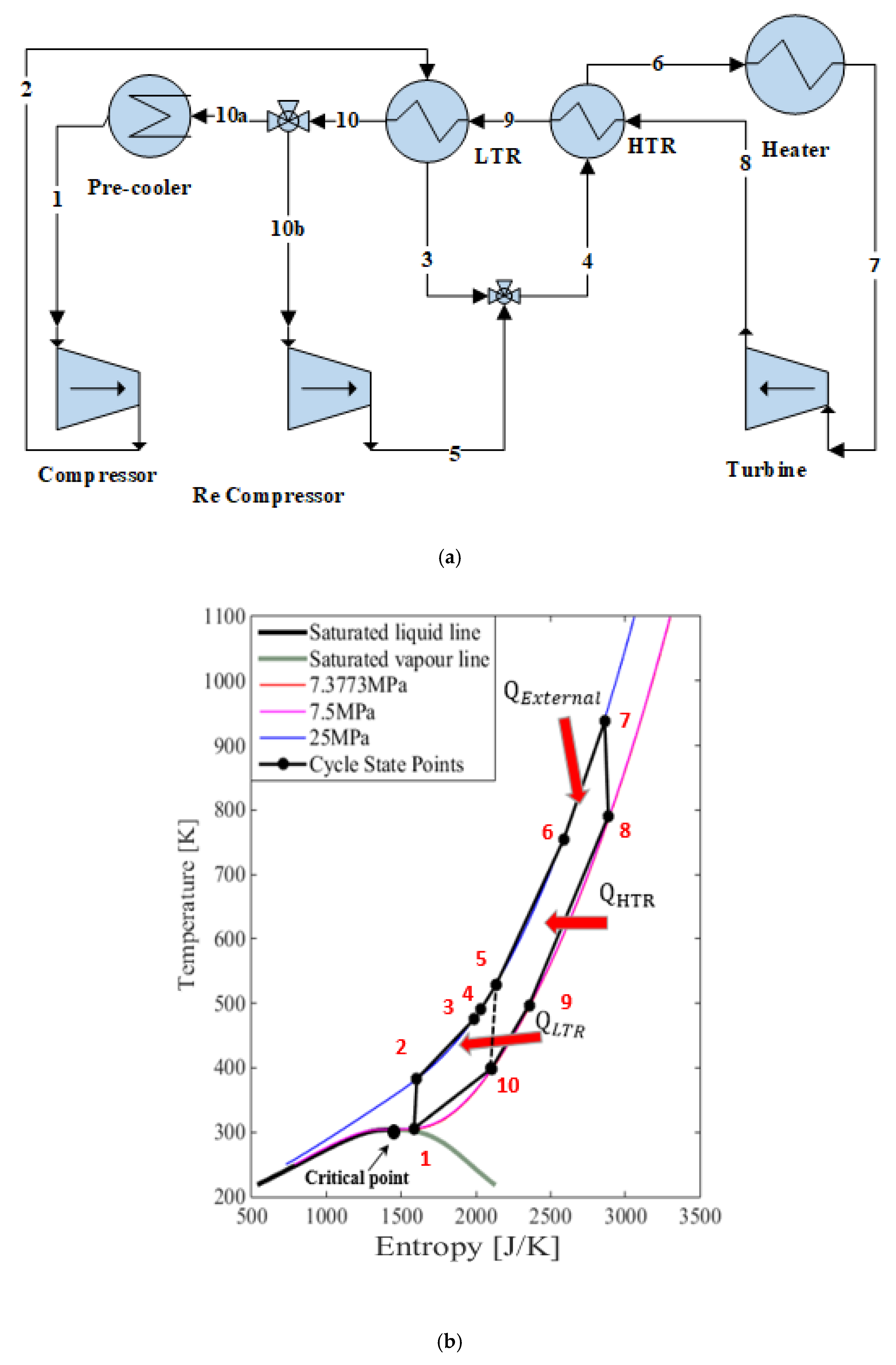
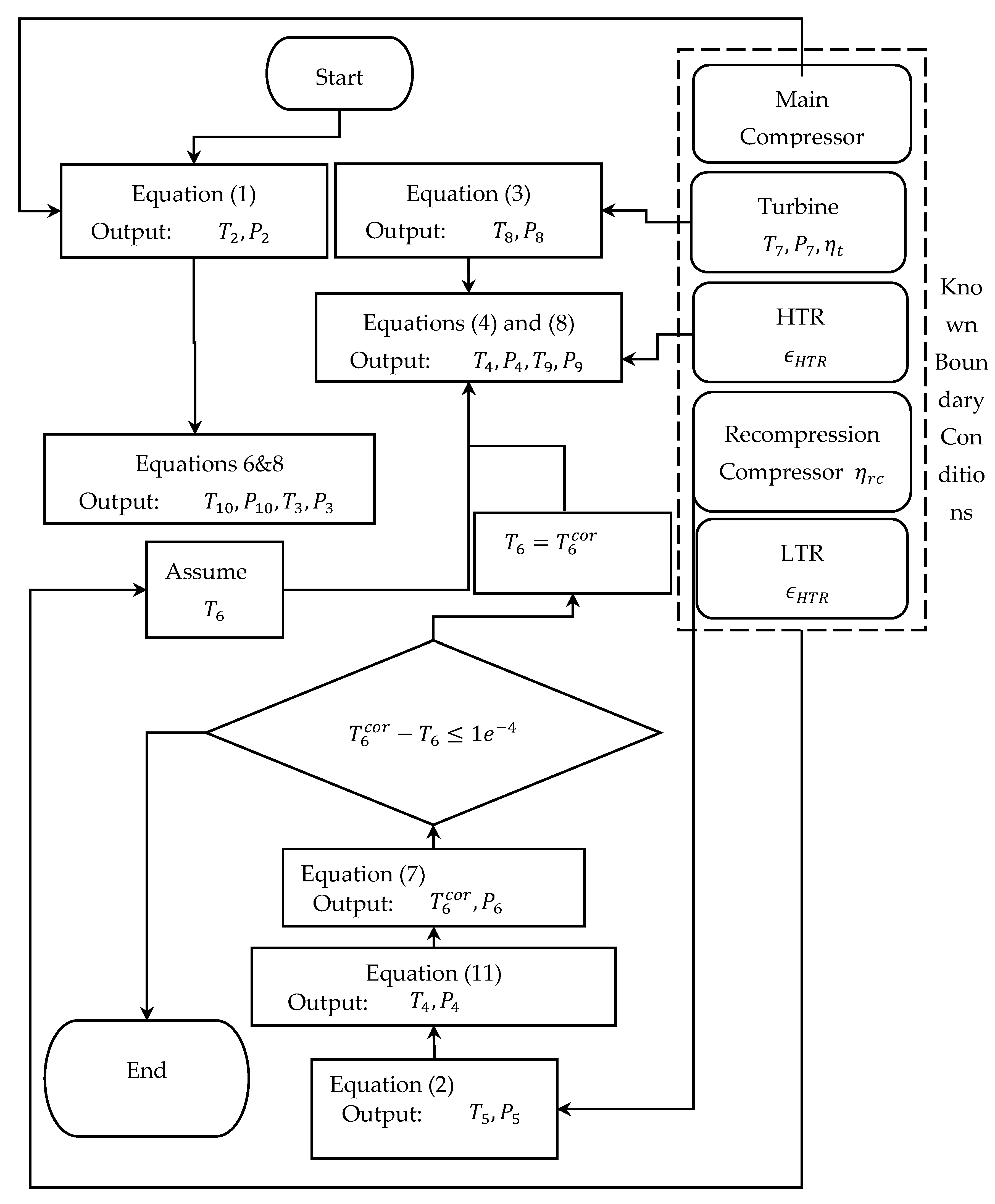
2.2. Model for Cycle Simulation and Analysis Code (CSAC)

The current section provides a mathematical model for the design point analysis of the recompression supercritical carbon dioxide cycle $(sC{O}_2-BC$) as shown in Figure 4. The major components of the recompression $sC{O}_2-BC$ is a turbine, two compressors (a main and a recompressor), two internal heat exchangers (LTR and HTR), a primary heat exchanger or heater, and a pre-cooler as shown in Figure 4. High-pressure fluid (state 6) gets heated from the heater (state 6–7). It gets expanded in the turbine (state 7–8), and during the expansion process, shaft work $\left(W_T\right)$ is obtained. After expansion, its temperature is still considerably high, as can be seen from Figure 4b. Therefore, to recuperate the valuable heat to the high-pressure side of the cycle, it passes first through the high-temperature recuperator (HTR) (state 8–9) and then flows through the low-temperature recuperator (LTR) (state 9–state 10). It should be noted here that before entering, the pre-cooler flow is split into two streams. A fraction (x) is sent to the recompressor (state 10–10b) while the remaining fraction (1–x) passes through the pre-cooler (state 10a–1). After the pre-cooler flow gets compressed in the main-compressor (state 1–2) gets heated from the LTR (state 2–3) and then combines with the flow coming from the re-compressor. Now the flow gets heated first in HTR (state 4–6) and then from the heater again for the next cycle.

To model high-temperature and low-temperature recuperators, PCHE-DAC was used in the heat exchanger model. The heat exchanger model is flexible and able to use any channel geometry; however, zigzag and straight-channel designs were utilized in the existing work. The model was coded in the MATLAB© environment, and the flow chart of the code is shown in Figure 5. To obtain the thermodynamic properties of $sC{O}_2$ REFPROP [36] was coupled with MATLAB through a function code at different states of the cycle.

2.2.1. Turbomachinery Models

In the literature [37], turbomachinery modeling is based on the turbine and compressor’s single equation relations, using isentropic efficiencies and pressure ratio information. In the current study, isentropic efficiencies (

Table 4. Components’ parameters used for the cycle simulation.

Parameters	Values
Compressor inlet Temperature ($T_1$) $\left[K\right]$	308
Compressor inlet pressure ($P_1$) [kPa]	7500
Cycle pressure ratio ($Pr$)	3.2
Turbine inlet temperature $\left(T_7\right)\left[K\right]$	1073

) are estimated using the Balje chart [38]; a non-isentropic compression and expansion process has been modeled using the following relations.

$$h_2=\frac{h_{2s}-h_1}{{\eta }_c}+h_1$$

(27)

$$h_5=\frac{h_{5s}-h_{10}}{{\eta }_{rc}}+h1$$

(28)

$$h_8=h_7-{\eta }_T\left(h_7-h_{8s}\right)$$

(29)

2.2.2. Recuperator Models

The heat exchanger models explained earlier are recuperator models. Assuming that both PCHEs are fully shielded for heat losses to surroundings, the energy conservation equation for the LTR and HTR is given by Equations (30) and (31).

$$h_9= h_8-\left(h_6-h_4\right)$$

(30)

$$h_{10}=h_9-\mathrm{x} \left(h_3-h_2\right)$$

(31)

$$\mathrm{x}= \frac{{\dot{m}}_c}{\dot{m}} \mathrm{where} \dot{m}={\dot{m}}_c+{\dot{m}}_{rc}$$

(32)

where the split-mass-fraction (x) can be calculated utilizing the following equation under the assumptions of ideal mixing and splitting at corresponding values.

The mixing value is modeled using Equation (33) by considering an ideal mixing.

$$h_4=\mathrm{x} h_3+\left(1-\mathrm{x}\right)h_5$$

(33)

Pressure losses across all heat exchangers are modeled using the following relation, and cycle efficiency is given by Equation (34).

$$p_{out}= p_{in}\left(1-f\right)$$

(34)

$${\eta }_{cyc}=\frac{W_T {\eta }_m-\left(W_C+W_{RC}\right)/{\eta }_m}{q_{in}}$$

(35)

Definitions of $w_t$,$w_c, and w_{rc}$ are given by the following equations.

$$W_T=\left(h_7-h_8\right)$$

(36)

$$W_C=\mathrm{x}(h_2-h_1)$$

(37)

$$W_{RC}=\left(1-\mathrm{x}\right)(h_5-h_{10})$$

(38)

The power cycle’s selected boundary conditions are based on the literature review of boundaries for the recompression Brayton cycle [7] and are listed in Table 4. Cycle calculations under given conditions (Table 4) were simulated using a CSAC for different split fraction values “x”. Thermodynamics state properties were obtained by coupling the MATLAB code with the REFPROP.

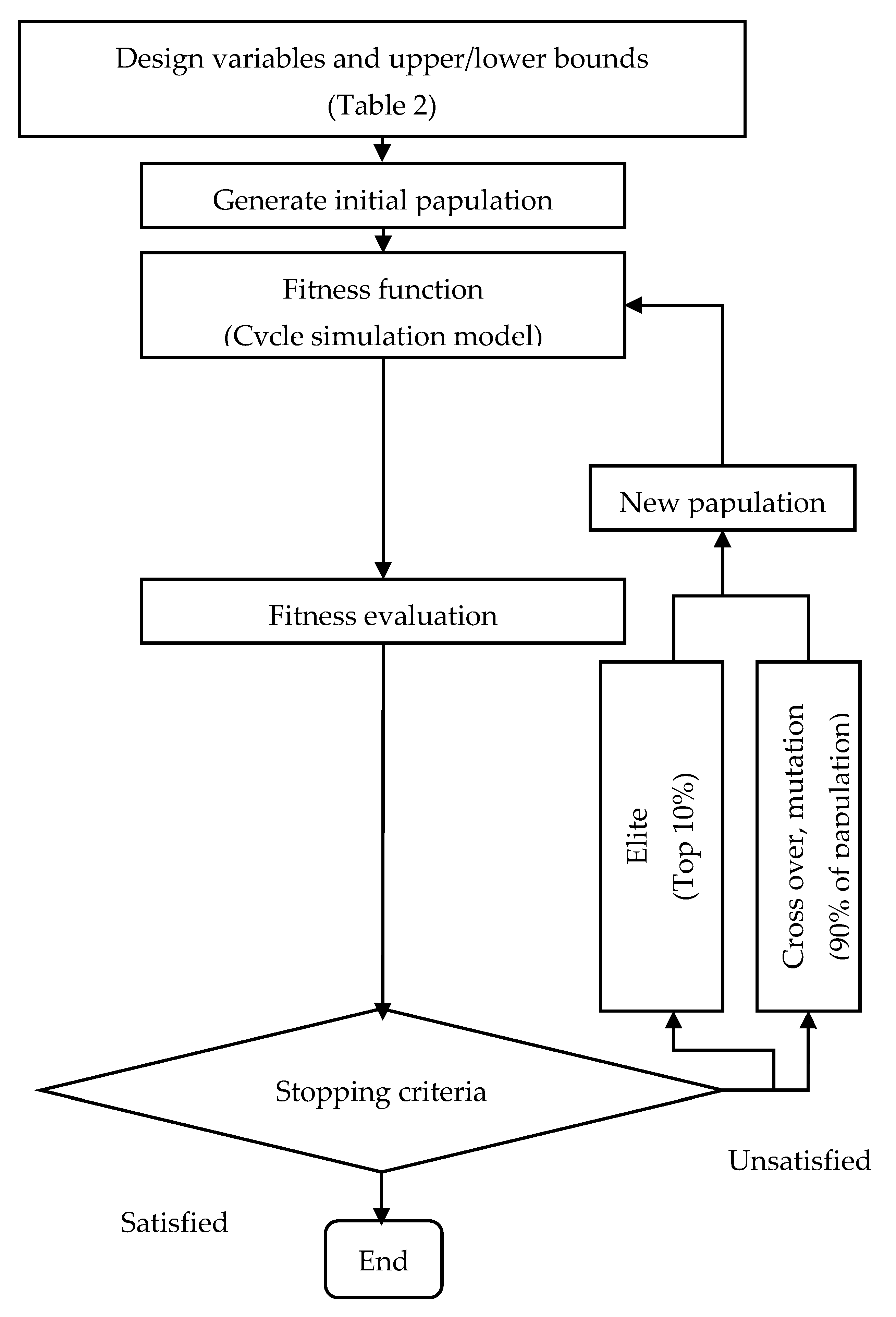
2.3. Heat Exchanger Optimization Based on Cycle Performance

For the PCHE optimization, four parameters were considered for the optimization process: $ϵ$, $Re$, channel configuration, and split mass fraction. The optimization method uses the genetic algorithm (GA). The design variables, including upper and lower bounds, are listed in

Table 5. Design variables employed for the current study with the upper and lower bounds.

Design Variable	Symbols	Upper Bounds	Lower Bounds
Effectiveness of the heat exchanger ($T_1$) $\left[K\right]$	x1	0.99	0.8
Inlet Reynolds number	x2	30,000	60,000
Split mass fraction	x3	0.50	0.95
Channel configuration	x4	Zigzag channel,	Straight-channel

. The GA has been frequently adopted in the literature [20,39,40,41,42,43] to solve global maximization and minimization problems. It is based on the stochastic method and uses the principle of survival of the fittest [39]. The GA is initialized through a random population of selected size based on the design variables chosen to define the first generation. The population is tested against the defined fitness function. The population in each generation improves through an iterative process using mutation, crossover, and elite selection. A schematic of the process is shown in Figure 6. The population size for the current study uses 100 combinations of the defined variables. For the values of the crossover fraction, mutation fractions for the current problem were chosen as 0.9 and 0.01. A 1% elite of the total population was carried forward unchanged to the next generation.

3. Result

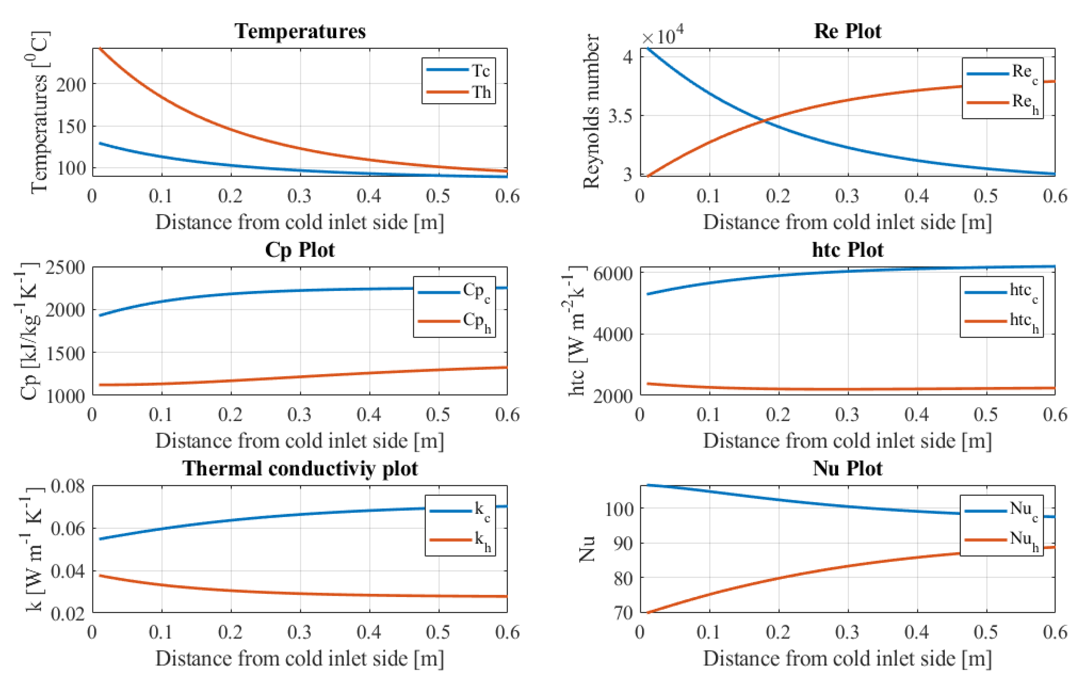
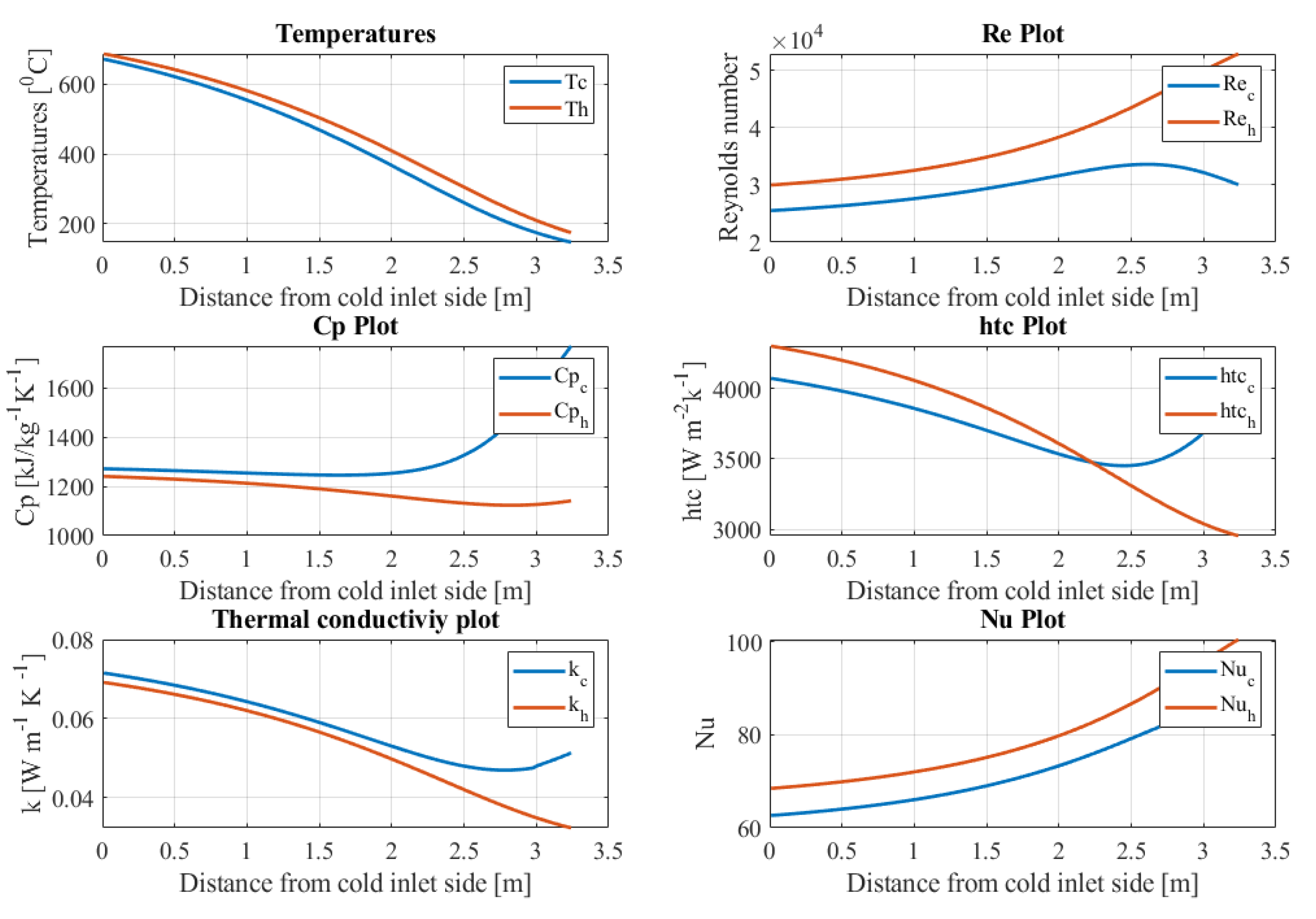
3.1. Characteristics of the PCHEs

The current study was conducted to evaluate the cycle’s performance and its components using zigzag and straight channels for the HTR and LTR. The research focuses mainly on discovering how operating conditions change across the different components of the cycle, i.e., turbine, compressor, and heat exchangers with zigzag and straight-channel geometries.

Figure 7 and Figure 8 show the profiles of temperature, Nusselt number ($Nu$), Reynolds number, specific heat capacity ($C_p$), thermal conductivity ($k$), and heat transfer coefficient ($h$) for high- and low-temperature recuperators under the cycle conditions given in Table 5. Figure 7 shows the LTR characteristics and suggests that the Reynolds number initially increases substantially along the length of PCHE before the curve flattens. In the cold side, the $Re$ increases along the PCHE’s length. Variations in the thermal conductivity, heat transfer coefficient, and thermal and specific heat capacity are as significant as variations in the Reynolds number. Furthermore, in Figure 7, the Nusselt number increases along the heat exchanger’s length on the hot side due to the increase in the Reynolds number. Figure 8 shows the characteristics of a high temperature recuperator (HTR). The HTR length is much longer than the LTR; variation in the working fluid properties along the length of the HTR is quite apparent. The temperature profiles in the heat exchanger are not linear that is quite interesting and help to avoid pinch point within the heat exchanger. The Reynolds number on the hot side increases along the heat exchanger’s length; on the cold side, the Reynolds number increases initially and starts decreasing after reaching the maximum value. The heat transfer coefficient’s value decreases along the heat exchanger’s length on the hot side; it decreases initially and then increases toward the end of the heat exchanger. In contrast, the Nusselt number increases along the heat exchanger’s length on both the hot and cold sides. It should be noted that the profiles of Reynold number, $htc$ and $Nu$ can be explained by the variation of the properties of carbon dioxide, based on its operation near the critical point. The variation in the specific heat capacity ($Cp$) and thermal conductivity ($k$) is shown in Figure 8. It shows that both $Cp$ and $k$ vary substantially along the heat exchange’s length due to temperature and pressure.

This section presents an assessment study for PCHEs with the straight-channel and zigzag-channel configurations. Temperature profiles along the length of the PCHE with straight-channel and zigzag-channel arrangements designed for the same heat load are shown in Figure 9. It can be seen that the size of the heat exchanger computed by the heat exchanger design code (PCHE-DAC) is three times longer for the LTR with a straight-channel configuration than with a zigzag-channel configuration. Furthermore, Figure 9 demonstrates the pressure drop variations across the PCHE with different design values for $Re$, $ϵ$, and channel’s geometry (zigzag or straight). Interestingly, the pressure drop across the PCHEs with the straight-channel is significantly higher than PCHEs with zigzag-channels even though the former’s friction factor is substantially higher than the latter (2–2.5 times). This can be explained by examining the data displayed in Figure 9, Figure 10, Figure 11 and Figure 12. The channel’s computed length for a certain channel’s configuration is greatly reliant on heat transfer characteristics linked with that certain channel configuration. In contrast, the pressure drop is linked with the pressure coefficient and the calculated length of the channel for a certain channel configuration.

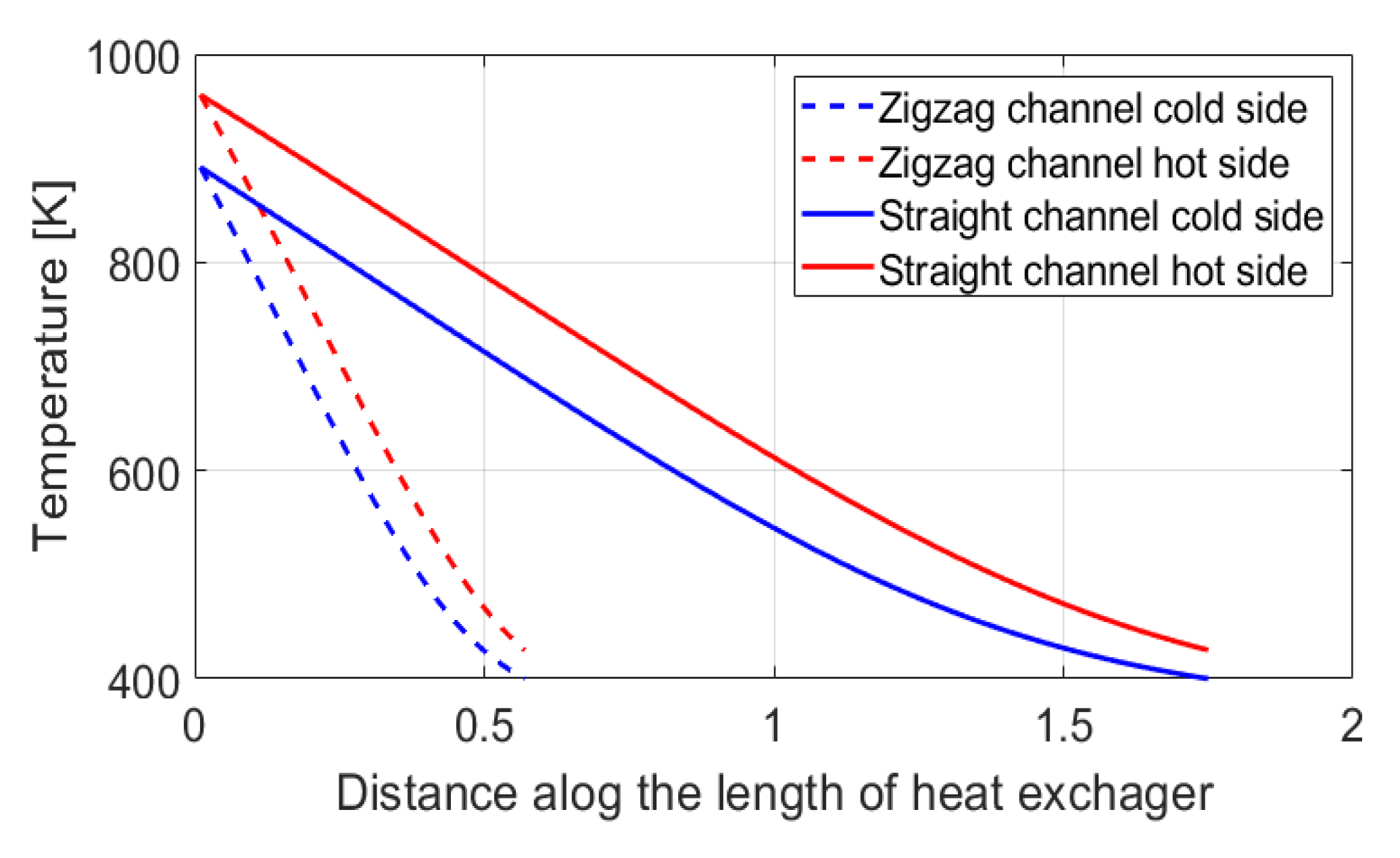
Comparison of Heat Exchanger Designs with Straight and Zigzag Channels

The data displayed in Figure 10 reflects Nusselt number values for the zigzag-channel geometry are comprehensively enhanced compared to the corresponding values for the straight-channel configuration. The Nu for the zigzag-channel is 2.5–3.5 times higher than the straight-channel geometry. That is why the zigzag-channel requires considerably shorter lengths to transfer similar values of the heat when ϵ is same for both configurations. Figure 13 shows that the length of the PCHEs with zigzag channels is 2–4 times less for various values of ϵ and Reynolds number. Based on the above discussion, it can be concluded that pressure losses across straight-channel geometry are dominated by longer channel lengths (3 to 4 times) rather than lower friction factor value (e.g., 2–2.5). This is the reason pressure losses in PCHEs with straight channels are higher in comparison with zigzag-channels

Figure 11 demonstrates $\mathsf{\Delta }P$ for PCHEs designed for different $R{e}_{in}$, $ϵ$, and channel shapes (zigzag or straight). For the both zigzag and straight-channel configurations, PCHE’s length increases with increasing Re. The increasing trend in PCHE’s length with $Re$ is understandable as it increases the mass flow rate that in turn would require more surface area if $ϵ$ is fixed. Alternatively, increase in the design value of $ϵ$ would increase the PCHE’s length as now again it would require more heat to be transferred to bring the difference in the exit temperature of hot and cold side further close. Consequently, pressure losses across the channel being a direct function of channel’s length would increase as well. Therefore, an increase in the length of the channel with the design values of the inlet Reynolds number and effectiveness of the heat exchanger is the main reason for the rise in pressure drop. However, at any fixed designed values of the inlet Reynolds number and effectiveness, the pressure drop in a straight-channel configuration is almost three times greater than in a zigzag-channel configuration. The surge in the $\mathsf{\Delta }P$ with $Re$ is small at lower values (Re < 40,000). By contrast, at higher values of $Re$ (Re > 40 k), the pressure drop becomes highly sensitive to Re. Figure 12 shows the variation in the pressure drop in the cold side of the PCHE. The pressure drop increases significantly with increasing Re and $ϵ$ for all channel designs. An increase in the pressure drop in the cold side with Re follows the same trend observed on the hot side. However, unlike the hot side of the PCHE, the pressure drop across the straight-channel geometry is less than $\mathsf{\Delta }P$ for the straight-channel and is only slightly greater than $\mathsf{\Delta }P$ for the zigzag channel.

Figure 13 shows the heat exchanger size variation for heat exchangers with different design values for Re, $ϵ$, and channel configuration (zigzag or straight). It is observed in the figure that the PCHE’s size decreases sharply with an increase in the $R{e}_{in}$ values for all $ϵ$ values and both channel configurations. However, once $Re$ exceeds 40,000, the decrease in the size of the heat exchanger with $Re$ becomes minimal. It is evident from Figure 10 that all curves relating to various values of $ϵ$ and both channel geometries become relatively flattered for $Re>40,000$. It can be inferred from Figure 10, Figure 11, Figure 12 and Figure 13 that Reynolds numbers ranging from $Re = 30,000$ to $Re = 40,000$ are appropriate for designing a heat exchanger that favors both the PCHE’s smaller size and lower pressure drop across it.

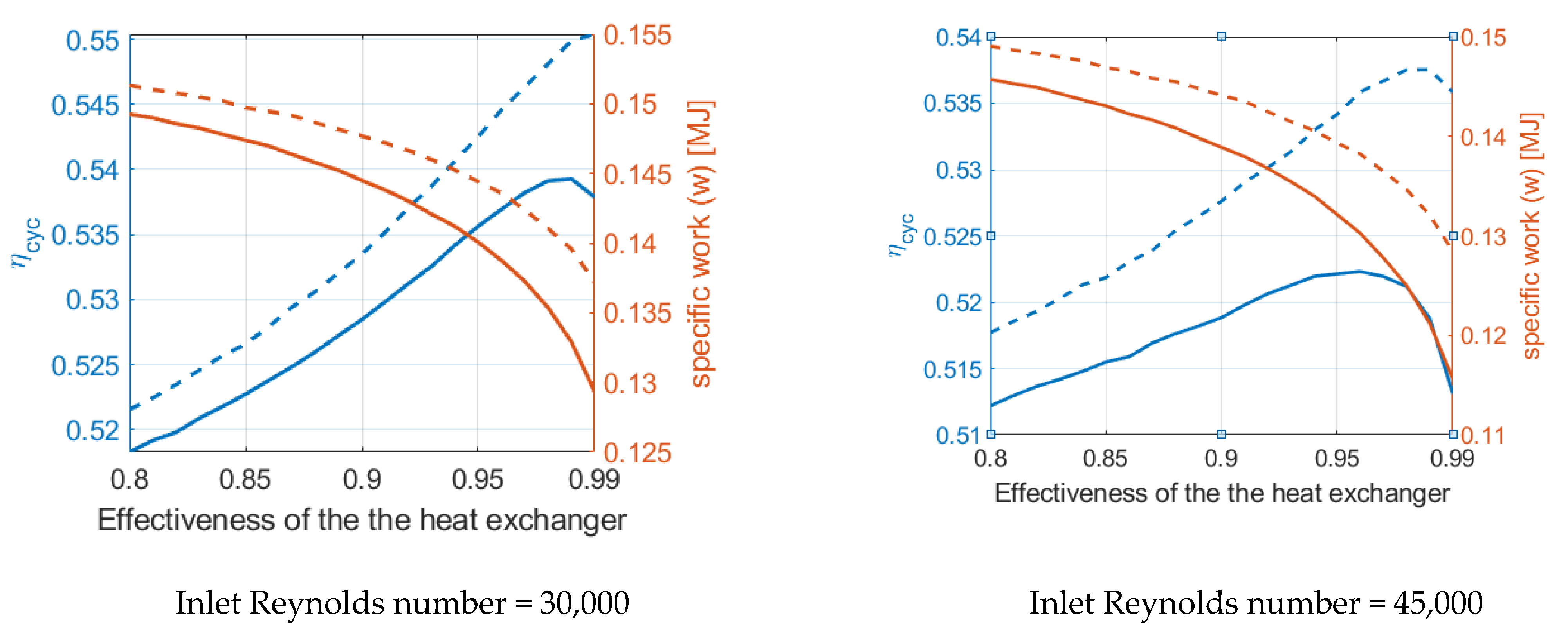
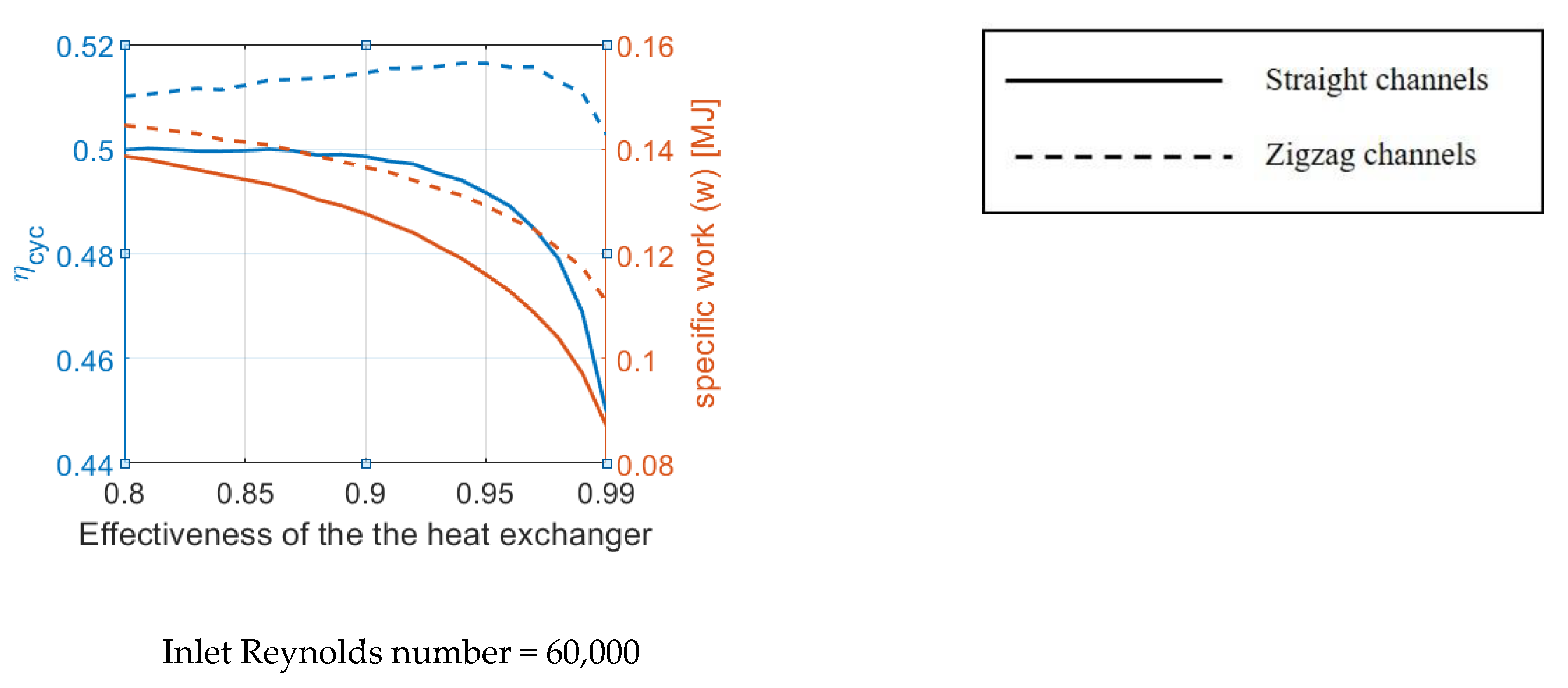
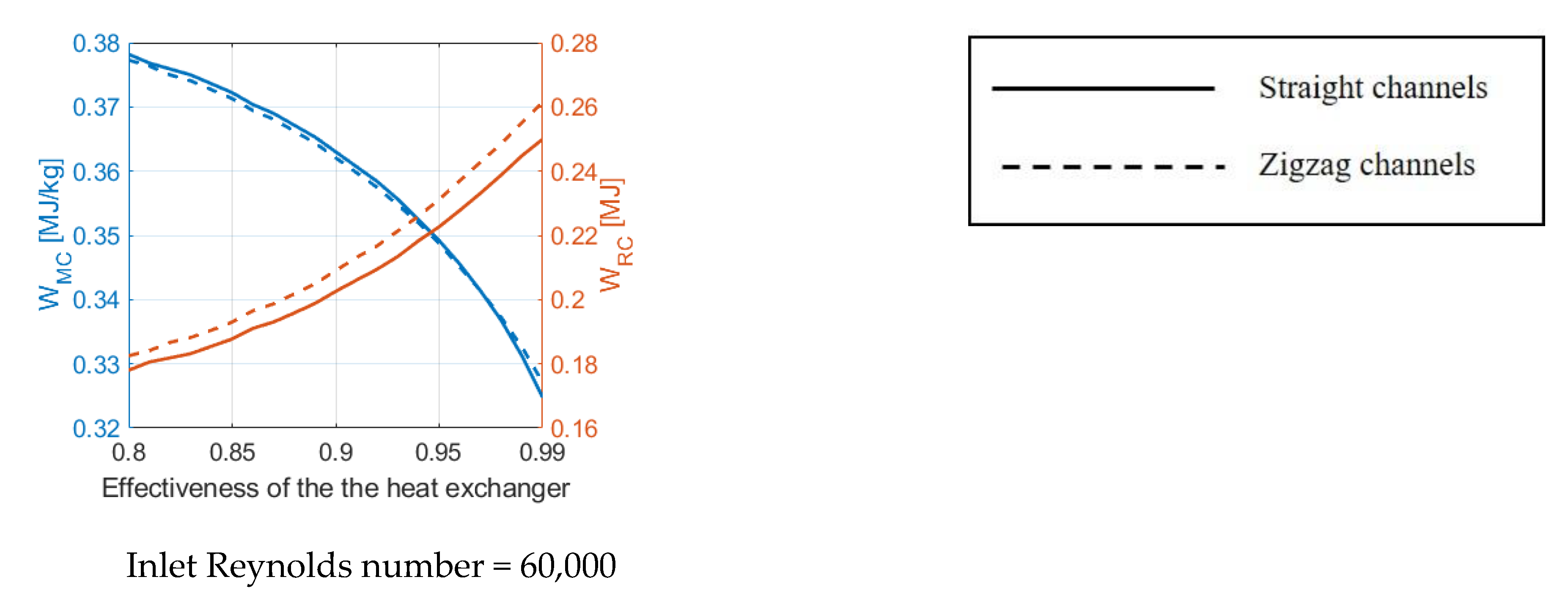
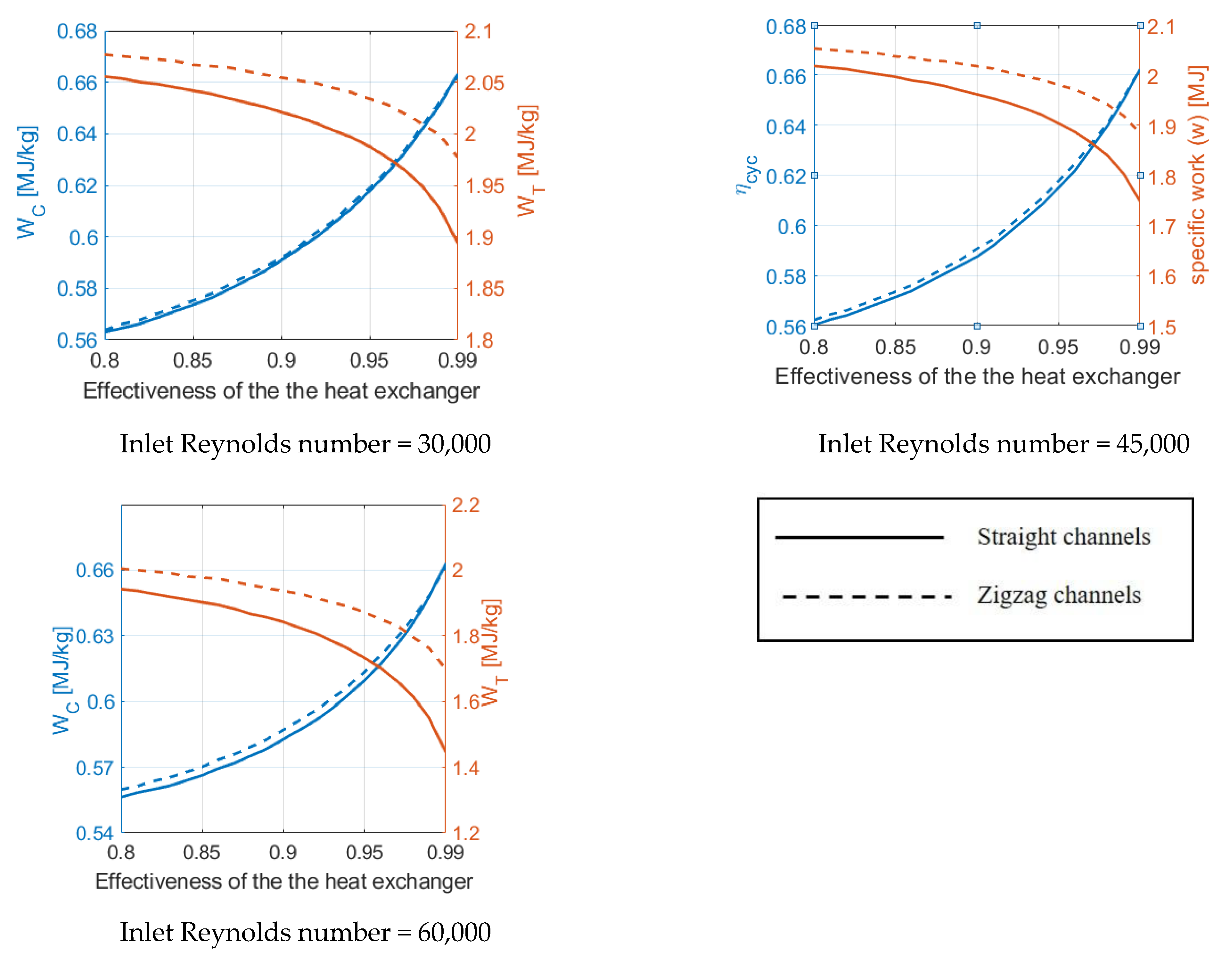
3.2. Cycle simulations Results

This section describes how the PCHE design is crucial to the cycle’s overall performance and the design of its turbomachinery components. Performance of the $sC{O}_2-BC$ was computed using different heat exchanger designs, as described earlier. Figure 14 shows the pressure ratio trend across the main compressor for heat exchangers with varying design values for Reynolds number, effectiveness, and channel configuration (zigzag or straight). It is observed in the figure that the pressure ratio across the main compressor does not change with modifications in the design. This is due to the imposed cycle’s boundary conditions dictating that the compressor’s inlet pressure and cycle pressure ratio remain constant. In contrast, the pressure ratio across the recompression compressor changes substantially with an increase in the design values of $ϵ, Re,$ and channel configuration. The pressure ratio for the recompression compressor (${\mathrm{Pr}}_{RC}$) decreases with an increase in $ϵ$. The slope of the ${\mathrm{Pr}}_{RC}$ lines become steeper as the heat exchanger’s effectiveness increases, dictating that the pressure ratio across the compressor declines sharply when $ϵ>0.95$. In Figure 14, the ${\mathrm{Pr}}_{RC}$ values are relatively higher for heat exchanger designs with higher inlet Reynolds number. However, recompression load is significantly higher on the recompressor for cycle layouts using PCHEs with straight-channel configurations. The load increases further if the heat exchanger designs have higher design values of $ϵ$ and Re.

Figure 15 shows the variation in the turbine’s pressure ratio profiles for heat exchangers with different design values for $Re, ϵ,$ and channel geometry (zigzag or straight). The figure suggests that the pressure ratio across the turbine decreases substantially with an increase in heat exchanger effectiveness. Heat exchanger designs with higher inlet Reynolds number experienced a greater decrease in $P{r}^T$ with $ϵ$. Comparison between zigzag and straight-channel configurations suggests that $P{r}^T$ for a heat exchanger with a zigzag-channel is significantly higher than with a straight-channel configuration. Figure 13 also shows the variation in the split mass values for different heat exchanger designs. The $x$ value decreases in heat exchanger designs with higher effectiveness. There is no appreciable change in the split mass fraction with varying inlet Reynolds number or channel’s shape.

Figure 16 demonstrates that the variation in ${\eta }_{cyc}$ and specific work of the cycle for PCHE designs. For a PCHE design with a low inlet Reynolds number, i.e., Re = 30,000, the ${\eta }_{cyc}$ increases substantially with a rise in the $ϵ$ with a zigzag-channel configuration. For straight channels, the ${\eta }_{cyc}$ deteriorates once $ϵ>0.97$. The specific work decreases appreciably for both channel geometries as the design value of $ϵ$ increases. For heat exchanger designs with Re = 45,000, ${\eta }_{cyc}$ initially increases with $ϵ$, then decreases after a certain value of effectiveness, $ϵ\approx 0.96$ and 0.98 for PCHEs with the straight-channel and zigzag-channel configurations, respectively. Furthermore, ${\eta }_{cyc}$ trends for PCHEs designs with Re = 60,000 are significantly different than with Re = 30,000 and 45,000. The ${\eta }_{cyc}$ increases decline sharply with $ϵ$ for heat exchanger designs with straight-channel configurations.

For heat exchanger design with zigzag-channel configurations, ${\eta }_{cyc}$ values increase slightly, with $ϵ$ ranging from 0.8 to 0.9. For $ϵ>0.93$, the value of ${\eta }_{cyc}$ decreases sharply with a further increase in the $ϵ$ of the PCHE. Trends of specific work with $ϵ$ are almost identical for all values of Re. The specific-work for heat exchanger designs with a straight-channel configuration is significantly smaller than with a zigzag-channel configuration. A similar trend is observed for PCHE designs with different values for the inlet Reynolds number.

Figure 17 suggests that the main compressor power increases considerably with an increase in $ϵ$. This could be explained by the split mass fraction decreasing with $ϵ$, reflecting that the mass flow rate through the main-compressor decreases, and thus also the size of the compressor and required power to run it. In contrast, the power required to run the recompression compressor increases faster than the decrease in the main compressor power. Thus, the total ability to run the compressor increases, despite the reduction in the main compressor power, as shown in Figure 17. A substantial increase in the main compressor power is attributed to the rise in the flow rate and pressure ratio across it with an increase in x with $ϵ$.

Figure 18 reflects the changes in the total compressor power and turbine power for heat exchangers with different design values for $Re, ϵ$ and channel’s geometry (zigzag or straight). The figure suggests that the total compressor power increases while the turbine power decreases with $ϵ$ for all values of the inlet $Re, ϵ$ and channel’s geometry (zigzag or straight). For all heat exchanger designs with different $ϵ$ and Re, $W_T$ values are higher for PCHEs using zigzag-channel configurations. However, the computed values of $W_C$ were almost identical for both channel configurations.

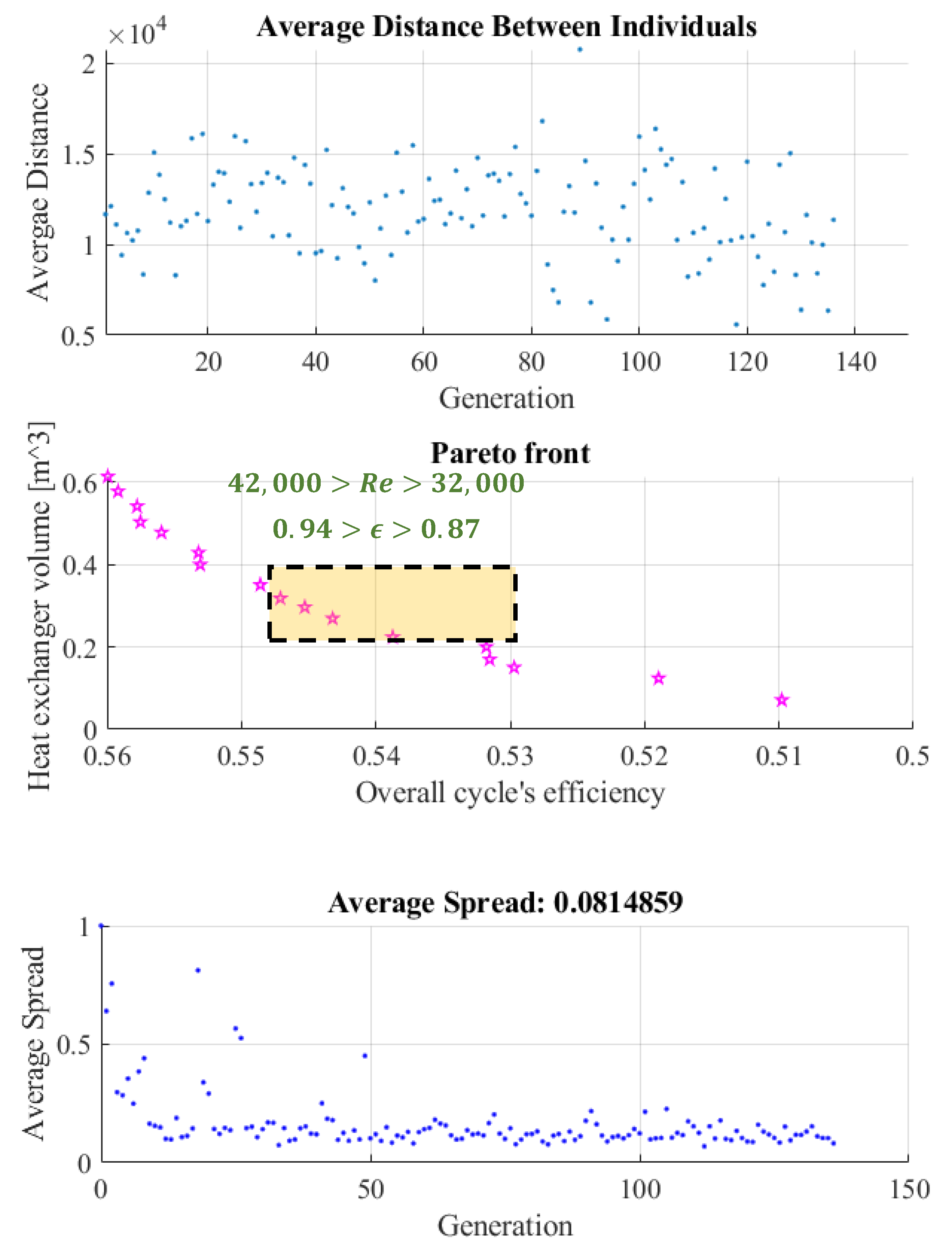
3.3. Heat Exchanger Optimization Results

Figure 19 shows PCHE optimization results and the convergence history; data for the final converged solution is presented in

Table 6. Converged generation data from Multi-objective genetic algorithm.

S. No.	$\mathit{ϵ}$	x	Re	Channel Configuration	${\mathit{\eta }}_{\mathit{c}\mathit{y}\mathit{c}}$	Volume
1.000	0.989	0.714	25,250.4	Zigzag-channel	0.560	0.614
2.000	0.989	0.714	25,250.4	Zigzag-channel	0.560	0.614
3.000	0.947	0.756	28,404.9	Zigzag-channel	0.547	0.318
4.000	0.969	0.731	28,382.4	Zigzag-channel	0.553	0.400
5.000	0.958	0.733	28,769.8	Zigzag-channel	0.549	0.351
6.000	0.986	0.716	25,454.2	Zigzag-channel	0.559	0.578
7.000	0.941	0.749	32,573.3	Zigzag-channel	0.543	0.270
8.000	0.811	0.798	32,479.6	Zigzag-channel	0.519	0.124
9.000	0.968	0.726	26,006.3	Zigzag-channel	0.553	0.429
10.000	0.931	0.769	36,265.9	Zigzag-channel	0.539	0.224
11.000	0.900	0.762	32,191.4	Zigzag-channel	0.532	0.201
12.000	0.800	0.825	58,820.2	Zigzag-channel	0.510	0.071
13.000	0.979	0.724	25,540.3	Zigzag-channel	0.558	0.504
14.000	0.870	0.796	31,450.6	Zigzag-channel	0.532	0.170
15.000	0.946	0.743	30,291.1	Zigzag-channel	0.545	0.297
16.000	0.889	0.783	41,244.1	Zigzag-channel	0.530	0.150
17.000	0.981	0.721	27,993.8	Zigzag-channel	0.556	0.478
18.000	0.983	0.715	25,414.4	Zigzag-channel	−0.558	0.542

. All converged solutions in the Pareto front are for the zigzag-channel geometry, attributed to the superior thermal characteristics associated with the zigzag-channel geometry. Minimum and maximum heat exchanger sizes were 0.07 m³ and 0.614 m³, respectively, corresponding to 53% and 56% overall efficiencies of the power cycle. A 3% increase in the cycle performance is at the expense of a nine-fold increase in the heat exchanger size. Considering the fact that most of the layout size for the $sC{O}_2-BC$ comes from the heat exchanger [29], it can be rephrased that a 3% increase in the cycle performance comes at the cost of a nine-fold increase in the layout size, which considerably impacts the initial cost. The region highlighted in Figure 17 also displays the optimal points from the Pareto front that offer a good compromise between the cycle performance and layout size for the $sC{O}_2-BC$. Figure 18 demonstrates the fluctuations in power consumed by the main compressor when the effectiveness was varied from 0.8 to 0.99 for different design values of the $Re\_in$ number (30k, 45k, and 60k) for straight and zigzag-channel configurations.

4. Conclusions

The current study was conducted to evaluate the effect of straight and zigzag-channel configurations on the overall performance of the $sC{O}_2-BC$ and its turbomachinery. To evaluate the different designs of the printed circuit heat exchanger, an in-house code was used for the PCHE design and analysis. The PCHE code was further used as a subroutine with a cycle design point analysis code to evaluate the effect of different PCHE designs on the cycle’s performance and its components, i.e., compressor and turbomachinery. The following conclusions were drawn from the study.

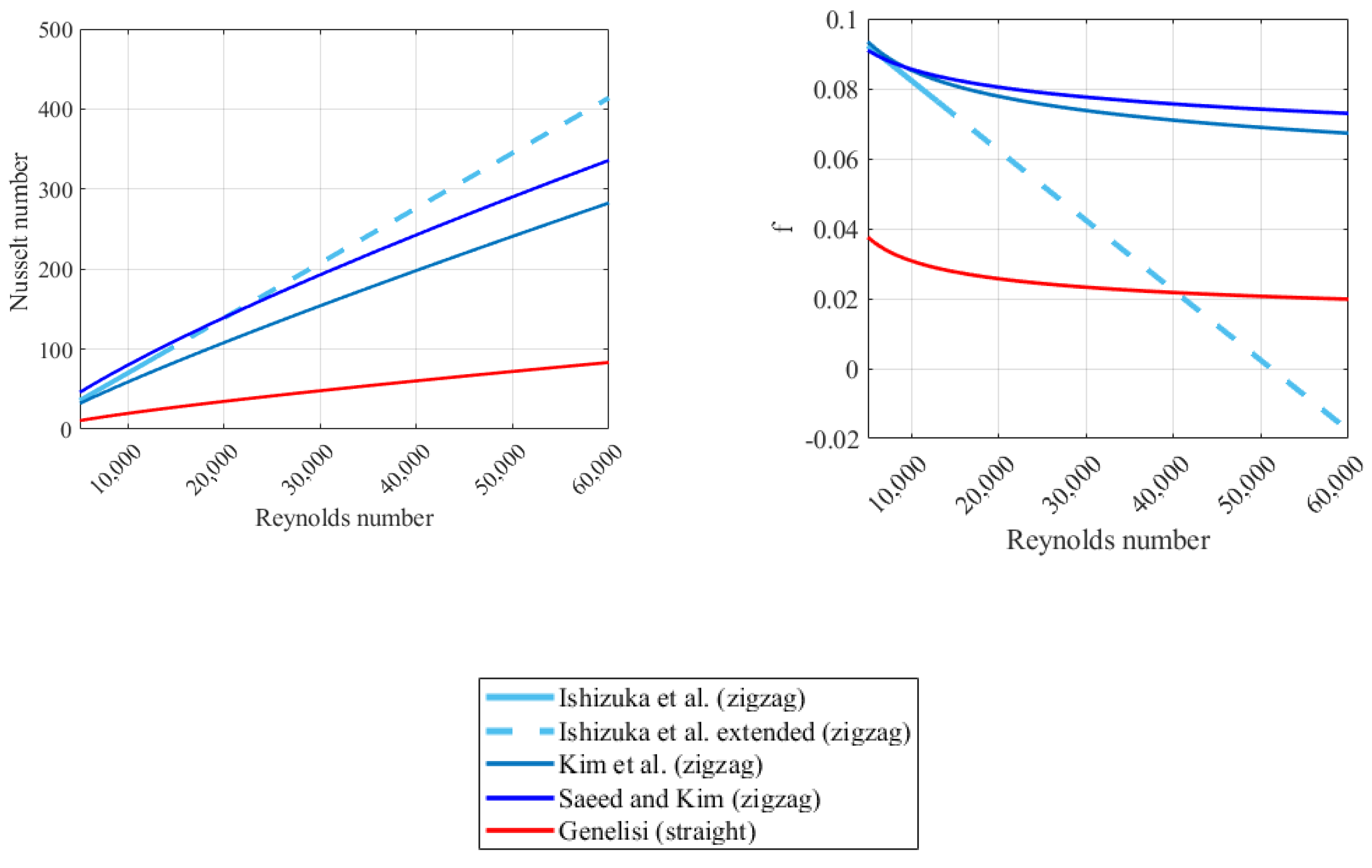
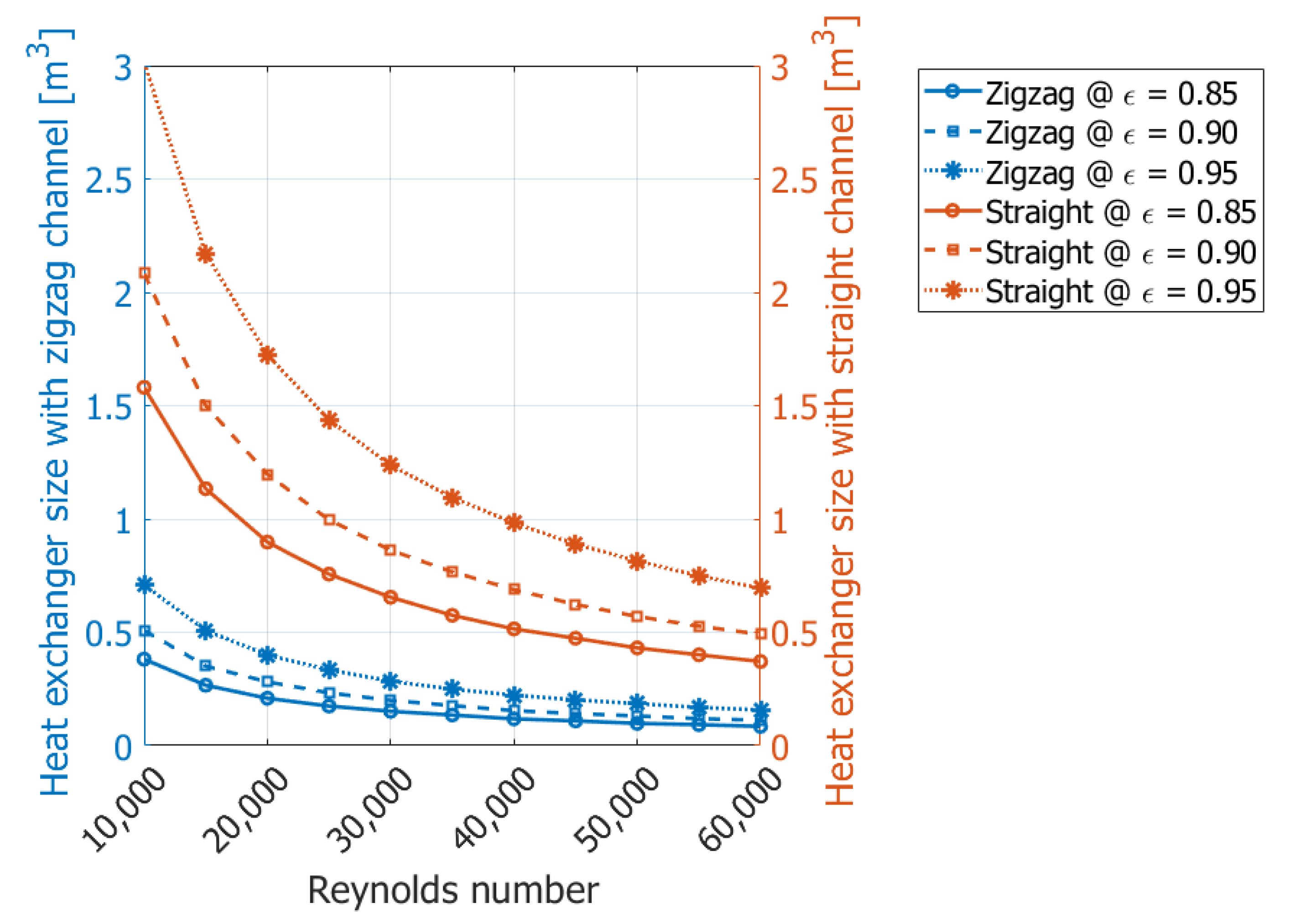
• For the same heat load, PCHEs with zigzag-channel configuration are computed to be approximately one third the size of PCHE with straight-channel configuration reasoned by the superior heat transfer characteristics associated with the zigzag channels. This in turn, reduces the pressure drop across the PCHEs with zigzag-channel in comparison with the PCHEs with straight-channel even though the friction factor for the latter is lower than the former.
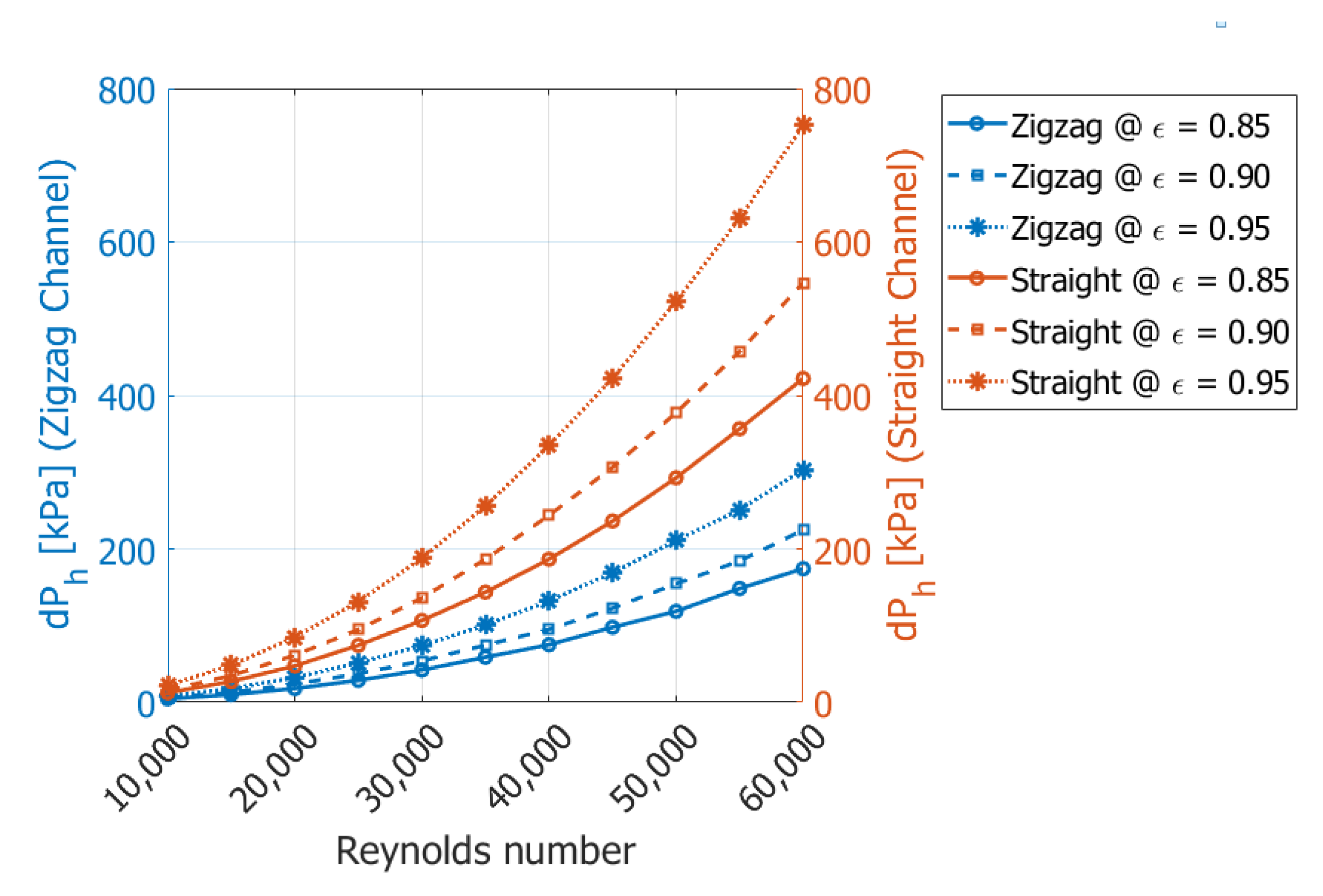
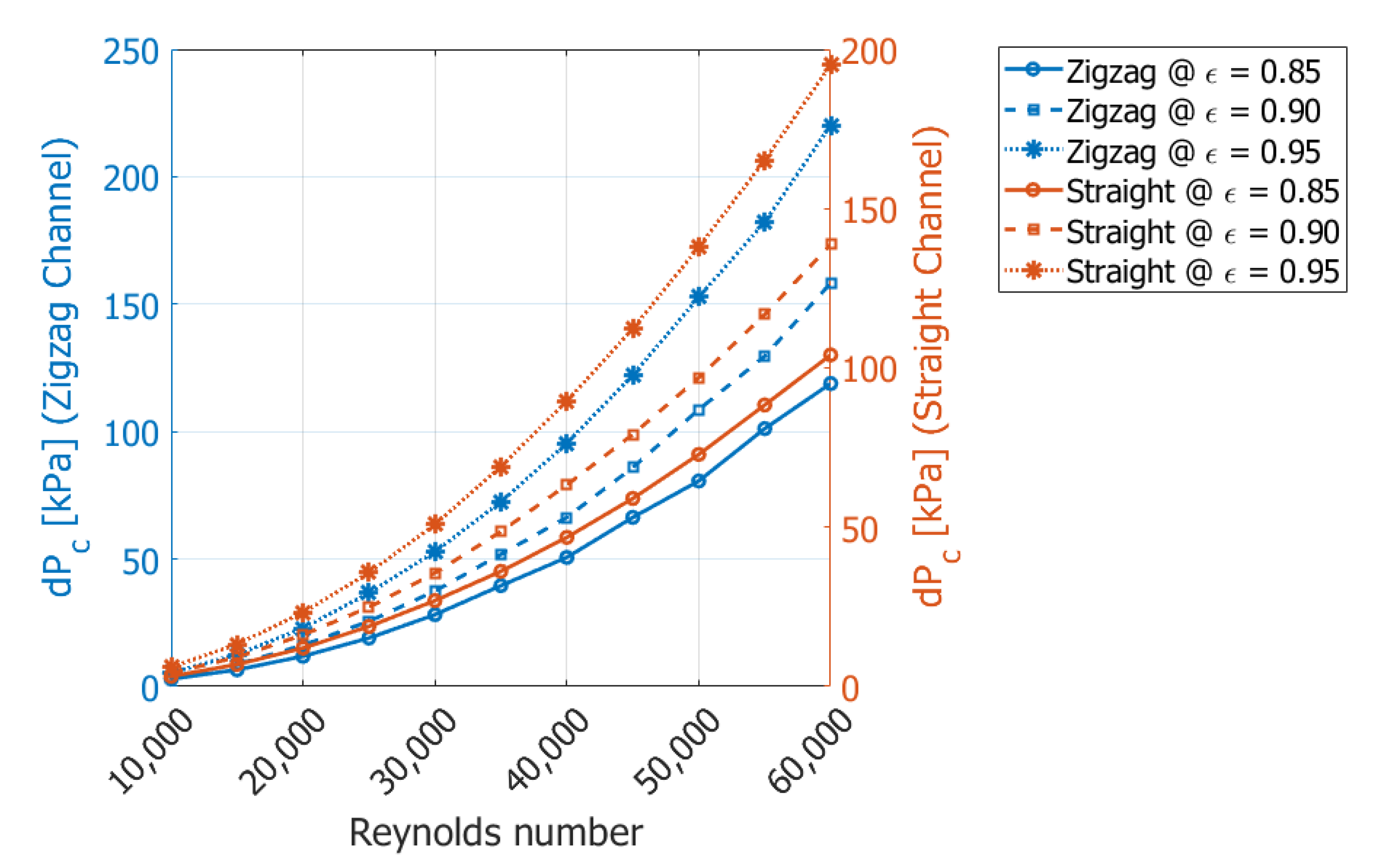
• For both channel configurations, the heat exchanger size increases with an increase in the design value for effectiveness. It decreases with a decrease in the design value for the inlet Reynolds number. The pressure drops increase by increasing both $ϵ$ and $Re$ in both hot and cold side channels of the heat exchanger and vice versa. The pressure drop for the PCHE on the cold side is only slightly higher for straight-channel geometry than for zigzag-channel geometry. However, the heat exchanger’s hot side’s pressure drop was three times higher for the straight-channel geometry than for the zigzag-channel geometry. Similar results were reported for the heat exchanger’s size by Saeed et al. [29]; however, they did not note the channel’s geometry’s effect on the component size.
• Due to the high-pressure drop in PCHEs with a straight-channel configuration, available pressure across the turbine is significantly smaller in the $sC{O}_2-BC$ than with a zigzag-channel configuration. Further load on the recompression compressor can be reduced significantly if PCHE designs with straight channels are replaced with zigzag-channels. In contrast, the main-compressor load was found to be independent of the PCHE design as inlet conditions were kept constant for the current study.
• PCHEs with a zigzag-channel configuration with design values for the inlet Reynolds number and heat exchanger effectiveness ranging from $32 \mathrm{k}$ to $42 \mathrm{k}$ and $0.94>ϵ>0.87$, respectively, are optimal for the $sC{O}_2-BC$ and provide a good compromise between cycle efficiency and layout size.

References

1. Brun, K.; Friedman, P.; Dennis, R. (Eds.) Fundamentals and Applications of Supercritical Carbon Dioxide (sCO2) Based Power Cycles; Woodhead Publishing: Sawston, UK, 2017. [Google Scholar]
2. Saeed, M.; Khatoon, S.; Kim, M.-H. Design optimization and performance analysis of a supercritical carbon dioxide recompression Brayton cycle based on the detailed models of the cycle components. Energy Convers. Manag. 2019, 196, 242–260. [Google Scholar] [CrossRef]
3. Manente, G.; Costa, M. On the Conceptual Design of Novel Supercritical CO2 Power Cycles for Waste Heat Recovery. Energies 2020, 13, 370. [Google Scholar] [CrossRef] [Green Version]
4. Ahn, Y.; Bae, S.J.; Kim, M.; Cho, S.K.; Baik, S.; Lee, J.I.; Cha, J.E. Review of supercritical CO2 power cycle technology and current status of research and development. Nucl. Eng. Technol. 2015, 47, 647–661. [Google Scholar] [CrossRef] [Green Version]
5. Feher, E.G. The supercritical thermodynamic power cycle. Energy Convers. 1968, 8, 85–90. [Google Scholar] [CrossRef]
6. Pham, H.S.; Alpy, N.; Ferrasse, J.H.; Boutin, O.; Quenaut, J.; Tothill, M.; Haubensack, D.; Saez, M. Mapping of the thermodynamic performance of the supercritical CO2 cycle and optimisation for a small modular reactor and a sodium-cooled fast reactor. Energy 2015, 87, 412–424. [Google Scholar] [CrossRef]
7. Turchi, C.S.; Ma, Z.; Neises, T.W.; Wagner, M.J. Thermodynamic study of advanced supercritical carbon dioxide power cycles for concentrating solar power systems. J. Sol. Energy Eng. 2013, 135, 375–383. [Google Scholar] [CrossRef]
8. Reyes-Belmonte, M.A.; Sebastián, A.; Romero, M.; González-Aguilar, J. Optimization of a recompression supercritical carbon dioxide cycle for an innovative central receiver solar power plant. Energy 2016, 112, 17–27. [Google Scholar] [CrossRef]
9. Al-Sulaiman, F.A.; Atif, M. Performance comparison of different supercritical carbon dioxide Brayton cycles integrated with a solar power tower. Energy 2015, 82, 61–71. [Google Scholar] [CrossRef]
10. Wang, J.; Wang, J.; Lund, P.D.; Zhu, H. Thermal Performance Analysis of a Direct-Heated Recompression Supercritical Carbon Dioxide Brayton Cycle Using Solar Concentrators. Energies 2019, 12, 4358. [Google Scholar] [CrossRef] [Green Version]
11. Khan, M.N.; Osman, M.; Alharbi, A.R.; Gorji, M.R.; Alarifi, I.M. Improving the efficiency of gas turbine-air bottoming combined cycle by heat exchangers and bypass control valves. Phys. Scr. 2020, 95, 45701. [Google Scholar] [CrossRef]
12. Chauhan, P.R.; Kumar, K.; Kumar, R.; Rahimi-Gorji, M.; Bharj, R.S. Effect of Thermophysical Property Variation on Entropy Generation towards Micro-Scale. J. Non-Equilib. Thermodyn. 2019, 45, 1–17. [Google Scholar] [CrossRef] [Green Version]
13. Sarkar, J.; Bhattacharyya, S. Optimization of recompression S-CO2 power cycle with reheating. Energy Convers. Manag. 2009, 50, 1939–1945. [Google Scholar] [CrossRef]
14. Sharma, O.P.; Kaushik, S.C.; Manjunath, K. Thermodynamic analysis and optimization of a supercritical CO2 regenerative recompression Brayton cycle coupled with a marine gas turbine for shipboard waste heat recovery. Therm. Sci. Eng. Prog. 2017, 3, 62–74. [Google Scholar] [CrossRef]
15. Sarkar, J. Second law analysis of supercritical CO2 recompression Brayton cycle. Energy 2009, 34, 1172–1178. [Google Scholar] [CrossRef]
16. Crespi, F.; Gavagnin, G.; Sánchez, D.; Martínez, G.S. Supercritical carbon dioxide cycles for power generation: A review. Appl. Energy 2017, 195, 152–183. [Google Scholar] [CrossRef]
17. Conboy, T.; Wright, S.; Pasch, J.; Fleming, D.; Rochau, G.; Fuller, R. Performance characteristics of an operating supercritical CO2 Brayton cycle. J. Eng. Gas Turbines Power 2012, 134, 111703–111715. [Google Scholar] [CrossRef]
18. Coco-Enríquez, L.; Muñoz-Antón, J.; Martínez-Val, J.M. New text comparison between CO2 and other supercritical working fluids (ethane, Xe, CH4 and N2) in line-focusing solar power plants coupled to supercritical Brayton power cycles. Int. J. Hydrog. Energy 2017, 42, 17611–17631. [Google Scholar] [CrossRef]
19. Saeed, M.; Kim, M. Analysis of a recompression supercritical carbon dioxide power cycle with an integrated turbine design/optimization algorithm. Energy 2018, 165, 93–111. [Google Scholar] [CrossRef]
20. Li, H.; Su, W.; Cao, L.; Chang, F.; Xia, W.; Dai, Y. Preliminary conceptual design and thermodynamic comparative study on vapor absorption refrigeration cycles integrated with a supercritical CO2 power cycle. Energy Convers. Manag. 2018, 161, 162–171. [Google Scholar] [CrossRef]
21. Wang, K.; He, Y.L.; Zhu, H.H. Integration between supercritical CO2 Brayton cycles and molten salt solar power towers: A review and a comprehensive comparison of different cycle layouts. Appl. Energy 2017, 195, 819–836. [Google Scholar] [CrossRef]
22. Wang, X.; Liu, Q.; Lei, J.; Han, W.; Jin, H. Investigation of thermodynamic performances for two-stage recompression supercritical CO2 Brayton cycle with high temperature thermal energy storage system. Energy Convers. Manag. 2018, 165, 477–487. [Google Scholar] [CrossRef]
23. Song, J.; Li, X.; Ren, X.; Gu, C. Performance analysis and parametric optimization of supercritical carbon dioxide (S-CO2) cycle with bottoming Organic Rankine Cycle (ORC). Energy 2018, 143, 406–416. [Google Scholar] [CrossRef]
24. Muñoz, M.; Rovira, A.; Sánchez, C.; Montes, M.J. Off-design analysis of a Hybrid Rankine-Brayton cycle used as the power block of a solar thermal power plant. Energy 2017, 134, 369–381. [Google Scholar] [CrossRef]
25. Kim, Y.M.; Sohn, J.L.; Yoon, E.S. Supercritical CO2 Rankine cycles for waste heat recovery from gas turbine. Energy 2017, 118, 893–905. [Google Scholar] [CrossRef]
26. Luu, M.T.; Milani, D.; McNaughton, R.; Abbas, A. Analysis for flexible operation of supercritical CO2 Brayton cycle integrated with solar thermal systems. Energy 2017, 124, 752–771. [Google Scholar] [CrossRef]
27. Saeed, M.; Berrouk, A.S.; Salman Siddiqui, M.; Ali Awais, A. Effect of Printed Circuit Heat Exchanger’s Different Designs on the Performance of Supercritical Carbon Dioxide Brayton Cycle. Appl. Therm. Eng. 2020, 179, 115758. [Google Scholar] [CrossRef]
28. Saeed, M.; Berrouk, A.S.; Salman Siddiqui, M.; Ali Awais, A. Numerical investigation of thermal and hydraulic characteristics of sCO2-water printed circuit heat exchangers with zigzag channels. Energy Convers. Manag. 2020, 224, 113375. [Google Scholar] [CrossRef]
29. Salim, M.S.; Saeed, M.; Kim, M.-H. Performance Analysis of the Supercritical Carbon Dioxide Re-compression Brayton Cycle. Appl. Sci. 2020, 10, 1129. [Google Scholar] [CrossRef] [Green Version]
30. Ha, S.T.; Ngo, L.C.; Saeed, M.; Jeon, B.J.; Choi, H. A comparative study between partitioned and monolithic methods for the problems with 3D fluid-structure interaction of blood vessels. J. Mech. Sci. Technol. 2017, 31, 281–287. [Google Scholar] [CrossRef]
31. Gnielinski, V. New equations for heat and mass transfer in turbulent pipe and channel flow. Int. Chem. Eng. 1976, 16, 359–368. [Google Scholar]
32. Ishizuka, T.; Kato, Y.; Muto, Y.; Nikitin, K.; Tri, N.L.; Hashimoto, H. Thermal-hydraulic characteristic of a printed circuit heat exchanger in a supercritical CO2 loop. In Proceedings of the 11th International Topical Meeting on Nuclear Reactor Thermal-Hydraulics (NURETH-11), Avignon, France, 2–6 October 2005. [Google Scholar]
33. Kim, S.G.; Lee, Y.; Ahn, Y.; Lee, J.I. CFD aided approach to design printed circuit heat exchangers for supercritical CO2 Brayton cycle application. Ann. Nucl. Energy 2016, 92, 175–185. [Google Scholar] [CrossRef]
34. Saeed, M.; Kim, M.-H. Thermal-hydraulic analysis of sinusoidal fin-based printed circuit heat exchangers for supercritical CO2 Brayton cycle. Energy Convers. Manag. 2019, 193, 124–139. [Google Scholar] [CrossRef]
35. Saeed, M.; Kim, M.-H. Thermal and hydraulic performance of SCO2 PCHE with different fin configurations. Appl. Therm. Eng. 2017, 127, 975–985. [Google Scholar] [CrossRef]
36. Crespi, F.; Sánchez, D.; Rodríguez, J.M.; Gavagnin, G. Fundamental thermo-economic approach to selecting sCO2 power cycles for CSP applications. Energy Procedia 2017, 129, 963–970. [Google Scholar] [CrossRef]
37. Lee, J. Design Methodology of Supercritical CO2 Brayton Cycle Turbomachineries. In Proceedings of the ASME Turbo Expo 2012: Turbine Technical Conference and Exposition, Copenhagen, Denmark, 11–15 June 2016. [Google Scholar]
38. Wang, K.; He, Y.-L. Thermodynamic analysis and optimization of a molten salt solar power tower integrated with a recompression supercritical CO2 Brayton cycle based on integrated modeling. Energy Convers. Manag. 2017, 135, 336–350. [Google Scholar] [CrossRef]
39. Bahamonde Noriega, J.S. Design Method for s-CO2 Gas Turbine Power Plants Integration of Thermodynamic Analysis and Components Design for Advanced Applications; P&E-2530; Delft University of Technology: Delft, The Netherlands, 2012. [Google Scholar]
40. Zhang, X.; Sun, X.; Christensen, R.N.; Anderson, M.; Carlson, M. Optimization of S-Shaped Fin Channels in a Printed Circuit Heat Exchanger for Supercritical CO2 Test Loop. In Proceedings of the 5th International Supercritical CO2 Power Cycles Symposium, San Antonio, TX, USA, 29–31 March 2016. [Google Scholar]
41. Shen, X.; Yang, H.; Chen, J.; Zhu, X.; Du, Z. Aerodynamic shape optimization of non-straight small wind turbine blades. Energy Convers. Manag. 2016, 119, 266–278. [Google Scholar] [CrossRef] [Green Version]
42. Saeed, M.; Kim, M.-H. Heat transfer enhancement using nanofluids (Al2O3-H2O) in mini-channel heatsinks. Int. J. Heat Mass Transf. 2018, 120, 671–682. [Google Scholar] [CrossRef]
43. Saeed, M.; Kim, M. Numerical study on thermal hydraulic performance of water cooled mini-channel heat sinks. Int. J. Refrig. 2016, 69, 147–164. [Google Scholar] [CrossRef]
Figure 1. Discretized model of the printed circuit heat exchanger.
Energies 14 00062 g001
Figure 2. Flow diagram for the heat exchanger code.
Energies 14 00062 g002
Figure 3. Comparison of the temperature profiles computed using PCHE-DAC with the extracted temperature data from the computational fluid dynamics (CFD) analysis [3].
Energies 14 00062 g003
Figure 4. (a) Layout of the cycle (b) temperature entropy (T-S) diagram; TS diagram of the cycle s C O 2 B C .
Energies 14 00062 g004
Figure 5. Flow diagram for the cycle simulation model.
Energies 14 00062 g005
Figure 6. Schematic of a genetic algorithm.
Energies 14 00062 g006
Figure 7. HTR characteristics along its length.
Energies 14 00062 g007
Figure 8. LTR characteristics along its length.
Energies 14 00062 g008
Figure 9. Temperature profiles in hot and cold sides of the zigzag and straight-channel heat exchangers.
Energies 14 00062 g009
Figure 10. Comparison of Nusselt number and friction factor values for the zigzag and straight-channel configuration based on the published data.
Energies 14 00062 g010
Figure 11. Variation in the values of pressure drop across the hot fluid channel with the design values of the flow Reynolds number.
Energies 14 00062 g011
Figure 12. Variation in the values of pressure drop across the cold fluid channel with the design values of the flow Reynolds number.
Energies 14 00062 g012
Figure 13. Variation in the heat exchanger size with design values of the inlet Reynolds number.
Energies 14 00062 g013
Figure 14. Variation in pressure ratio of the main compressor and recompress with the effectiveness of the heat exchanger corresponding to different values of inlet Reynolds number.
Energies 14 00062 g014
Figure 15. Variation in the turbine’s pressure ratio and split mass fraction with the effectiveness of the heat exchanger corresponding to different values of inlet Reynolds number.
Energies 14 00062 g015aEnergies 14 00062 g015b
Figure 16. Variation in the cycle’s performance and specific work at different values with the effectiveness of the PCHES corresponding to various values of R e i n .
Energies 14 00062 g016aEnergies 14 00062 g016b
Figure 17. Variation in the main-compressor and compressor’s power with the effectiveness of the PCHE corresponding to different values of R e i n .
Energies 14 00062 g017aEnergies 14 00062 g017b
Figure 18. Total compressor’s work and turbine’s work profile with the ϵ of the PCHE corresponding to different values of R e i n .
Energies 14 00062 g018
Figure 19. PCHE optimization for the maximization of the cycle’s performance while keeping the size minimum.
Energies 14 00062 g019