2. Introduction
Bilateral contracts (BC) are arrangements between two parties. In an electricity market, these contracts are often established by a Generation Company (GC) and an Electricity Supplier Company (ESC) under a set of terms, including price, duration, and the volume of electricity to be delivered. The main objective of arranging a BC is to hedge against day-ahead (spot) market price volatility since this volatility has increased by the deregulation of the electric power industry [
1,
2].
Prior to BC settlement, both parties forecast prices in the spot market to determine their strategies under the BC and then, independently, schedule electricity deliveries at time intervals to maximize their profits. Once a BC is implemented, its parties are liable to follow the delivery schedule stipulated in it [
3,
4].
BCs and the spot market are related since one influences the prices and volumes negotiated in the other [
4]. If improperly chosen, a BC can have the opposite effect due to the spot price being too high or too low at the market-clearing time when compared to the contract price [
5].
Several works have already been published proposing strategies to deal with price risk [
6,
7,
8,
9,
10,
11], usually analyzing the interaction between BCs and ESCs applying game theory [
12,
13,
14,
15,
16,
17,
18]. In [
6], the efficient frontier is used as a tool to identify the preferred portfolio of contracts. In [
7] and [
8], methodologies for the development of bidding strategies for electricity producers in a competitive electricity marketplace are presented. These studies use the fact that market participants react to competitors’ strategies aiming to maximize their payoffs [
7]. Risk is introduced in market generation bidding in [
9] using a mean-variance method and uncertainty, whereas in [
10], a binary expansion approach is applied. In contrast, a dynamic stochastic cooperative exchange based on a bargaining scheme is used to establish contracts in [
11]. In [
12], the trading method is based on the non-cooperative Nash bargaining game in which each transaction and its optimal price are determined to optimize the interests of individual parties. In [
13], the authors use cooperative game theory to simulate the decision-making process for defining offered prices in a deregulated environment by creating coalitions. Authors in [
14] formulate a prisoner’s dilemma matrix Nash game to show that suppliers have an incentive to withhold capacity from the market shifting the aggregated supply curve to cause a price spike. Another Nash equilibrium game is set in [
15], analyzing power transactions in a deregulated energy marketplace where participants maximize their net profits through optimal bidding strategies. The same concept is applied in [
16] for bilateral electricity markets. Another model presented in [
17] uses a mathematical program with equilibrium constraints (MPEC) for a profit-maximizing problem for a generator bidding in a competitive electricity market. Finally, a general view of different market operations, considering forecasting, scheduling, and risk management, is presented in [
18].
While many of the aforementioned works focus on finding an optimum solution for only one of the parties, Palamarchuk proposed a different approach [
3]. The proposed approach aimed to achieve an arrangement equally beneficial for both parties, the BC, and the ESC. Moreover, [
3] implemented the Nash bargaining Solution (NBS) to obtain the relative concession to be made by both parties. In this work, it is shown that a better outcome than the NBS is possible by applying the Raiffa–Kalai–Smorodinsky (RKS) bargaining solution. Therefore, the research gap is based on the fact that the RKS bargaining solution has not yet been applied to BC contracts in electricity markets. When implementing the RKS bargaining solution, a lower concession is made by both the GC and the ESC. Moreover, we have considered previous research mainly related to the Nash Bargaining Solution (NBS). The RKS technique developed can be applied in the energy market, including the Bilateral Contract (BC) transactions among pairs of Electricity Supplier Companies (ESC) and Generation Companies (GC).”
This work has the novelty of implementing the RKS approach for a bargaining solution for bilateral contracts in electricity markets, as already stated. It considers two players, an Electricity Supplier Company (ESC) and a Generation Company (GC), where they achieve a compromise approach applying the Raiffa–Kalai–Smorodinsky (RKS) equilibrium having the goal of decreasing the concessions to be made related to their maximum possible profits. Once the RKS methodology is applied, considering not only the input data set (spot price scenarios and the demand for the end consumers), but also the production cost functions, the electricity generation limits, and the deliveries under the Bilateral Contracts (BC), the applied RKS approach achieves better results than the already applied Nash Bargaining Solution (NBS).
This paper is structured as follows.
Section 3 presents the background for the proposed RKS bargaining solution problem and introduces the notation and mathematical models used for BCs. In this section, the RKS compromise approach for BC scheduling is also discussed.
Section 4 presents the numerical results of the proposed RKS approach, and
Section 5 states the conclusions.
3. Materials and Methods
In order to implement the proposed model, the RKS bargaining solution, and its compromise approach, besides the notation used in this research, are presented in the next subsections. The bilateral contract model considered is also explained.
3.1. Raiffa–Kalai–Smorodinsky Bargaining Solution
In a cooperative game, two or more players look for an agreement that will be mutually beneficial. A bargaining solution is an equilibrium allocation to satisfy the parties giving them no reason to bargain further.
In 1950, Nash proposed a framework allowing a unique feasible outcome to be selected as the solution of a given bargaining problem. It was characterized by four axioms, namely Symmetry (SYM), Weak Pareto Optimality (WPO), Scale Invariance (SI), and Independence of Irrelevant Alternatives (IIA) [
19].
Kalai and Smorodinsky questioned the IIA axiom proposing a new solution. Their solution focused on the parties’ ideal payoffs, meaning the highest possible payoff that one side could achieve individually and introduced the monotonicity axiom as a substitute to the IIA axiom [
20,
21].
When the solution outcome does not respond to the changes in the bargaining set, that axiom is coined as the independence axiom. Furthermore, when at least one of the payoff solutions is altered following a change in the bargaining set, it is known as the monotonicity axiom [
19].
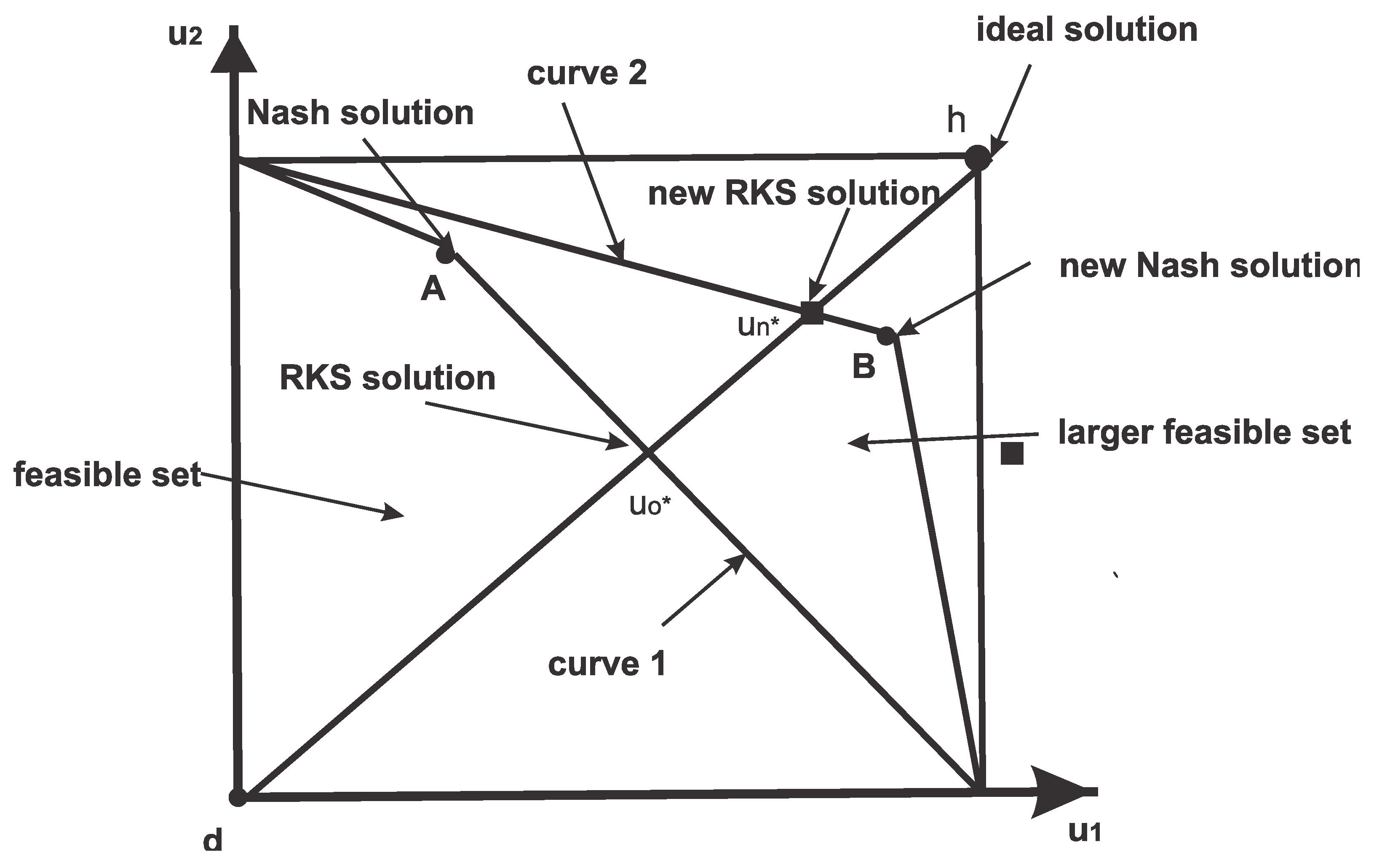
This approach initiated with a critique of the Nash bargaining solution since, even for a larger feasible set, the new Nash bargaining solution could yield a worse result [
20,
21]. When observing
Figure 1, a potential bargaining outcome expressed in units of utility can be represented by curve 1. Moreover, another potential bargaining outcome expressed also in units of utility can be represented by curve 2. Analyzing
Figure 1, even though curve 2 has a larger feasible set than curve 1, the Nash bargaining equilibrium would give as result point B for curve 2, making player 2 worse off compared with point A in curve 1. The solution obtained by the RKS approach when the feasible set increases is point
in curve 2, but is
in curve 1, making both players better off when applying the RKS approach (see
Figure 1). Therefore, the RKS bargaining solution is a Pareto optimal point from
d to the ideal solution,
h [
22,
23].
A larger feasible set with the same ideal solution, point
h, in
Figure 1, results in a bargaining solution better (or no worse) for all players when applying the RKS methodology. In summary, when the feasible set is represented by curve 1, RKS obtains the result given by point
; when the feasible set is curve 2, RKS obtains the new result, point
, which is better off (or no worse) for both players. Finally, as already stated, it can then be said that the RKS bargaining solution is a Pareto optimal point on the line from
d to the ideal solution,
h [
22,
23].
Therefore, the RKS bargaining solution is a Pareto optimal point within the line between
d and the ideal solution,
h. Then, the players receive an equal fraction of their possible utility gains given by:
3.2. Bilateral Contract Scheduling
By scheduling, we refer to the amount of electricity to be delivered at each time interval t throughout the contract duration [
3]. Each party, the GC and the ESC forecast the electricity price in the spot market and schedule the electricity deliveries to maximize their profit. The forecasts of electricity prices in the spot market at each time interval
t are random variables [
4].
Two types of BCs are considered:
Type I: The buyer (ESC) determines the electricity amount to be delivered under the BC at each time interval t. The supplier (GC) must guarantee electricity delivery in accordance with the buyer’s requirements. Thus, in a Type I contract, the ESC maximizes its expected profit, S1.
Type II: The supplier (GC) determines the electricity amount to be sold according to the contract at each time interval t. The buyer (ESC) accepts the delivered electricity according to the supplier decision, and in that case, the GC maximizes its expected profit, S2.
The following equations were introduced in [
3].
For a Type I contract, ESC’s profit (
S1) is given by:
where
E is the mathematical expectation symbol. Moreover,
J is the contract value considered as a constant since, in this work, the parties agree on a contract price in their BC. The profit maximization is equivalent to the maximization of the expected sales revenue,
R1, in the spot and retail markets:
subject to:
the total contract volume:
the sales to end consumers:
the delivery amount under contract at certain intervals:
the non-negativity of variables:
Once the ESC has solved the problem (Equations (3)–(7)) to schedule the electricity deliveries
xt,
t = 1,
..., N for the contract period, it will bring it to the attention of the GC. In that case, the GC agrees to supply electricity according to the schedule proposed by the ESC. Suppose that for each time interval
t the GC knows its production cost,
, as a function of the electricity generation,
, then, the production cost function is obtained based on the optimal unit commitment [
3].
For a Type II contract, the GC’s goal is to maximize its profit,
S2, by simultaneously trading in the spot market and in the BC market as represented by the following function:
Since
J is constant, Equation (8) is equivalent to:
subject to:
the electricity generation at each interval:
the delivery amount under the contract at individual intervals:
the non-negativity of variables:
A stochastic dynamic programming approach is applied to solve the problems mentioned above [
3]. Moreover, an increase in electricity delivery at an interval results in a decrease at the others. After having solved Equations (3)–(7) and Equations (9)–(12), a compromise approach can be applied where the RKS bargaining solution is achieved.
3.3. RKS Compromise Approach for BC Scheduling
A compromise approach for BC scheduling is a way to eliminate the advantage that the party making the delivery schedule would have over the other. This approach provides an opportunity to determine electricity deliveries that yield relative equal benefits for the parties. With this method, both parties can schedule deliveries together or by a neutral third party.
For the compromise approach, both parties must schedule their deliveries independently. If the ESC schedules deliveries
xt,
t = 1
,…, N independently, it solves the problem (Equations (3)–(7)) so it can obtain the maximum profit. When the GC schedules the deliveries
xt,
t = 1
,…, N independently, it should not follow any delivery schedule suggested by the ESC and, instead of constraint (Equation (11)) in Equations (9)–(12), it should consider:
and the amount deliveries under the BC at the intervals should obey:
When applying the RKS bargaining solution approach, the parties intend to maximize their revenues:
Or
Adding the constraint related to the RKS solution:
where
is the obtained value of the contract when Type I and II contract problems are solved, being given by
. The following conditions represented by Equations (17)–(23) must also be satisfied:
subject to:
Electricity generation at each interval:
Amount of deliveries under contract at certain intervals:
Non-negativity of variables:
The model applying the RKS bargaining solution is compared with the results applying the NBS in [
3]. It must be said that, when implementing the NBS, the objective function applied minimizes the concessions of each player in the game, represented by
k:
also,
k is equal to:
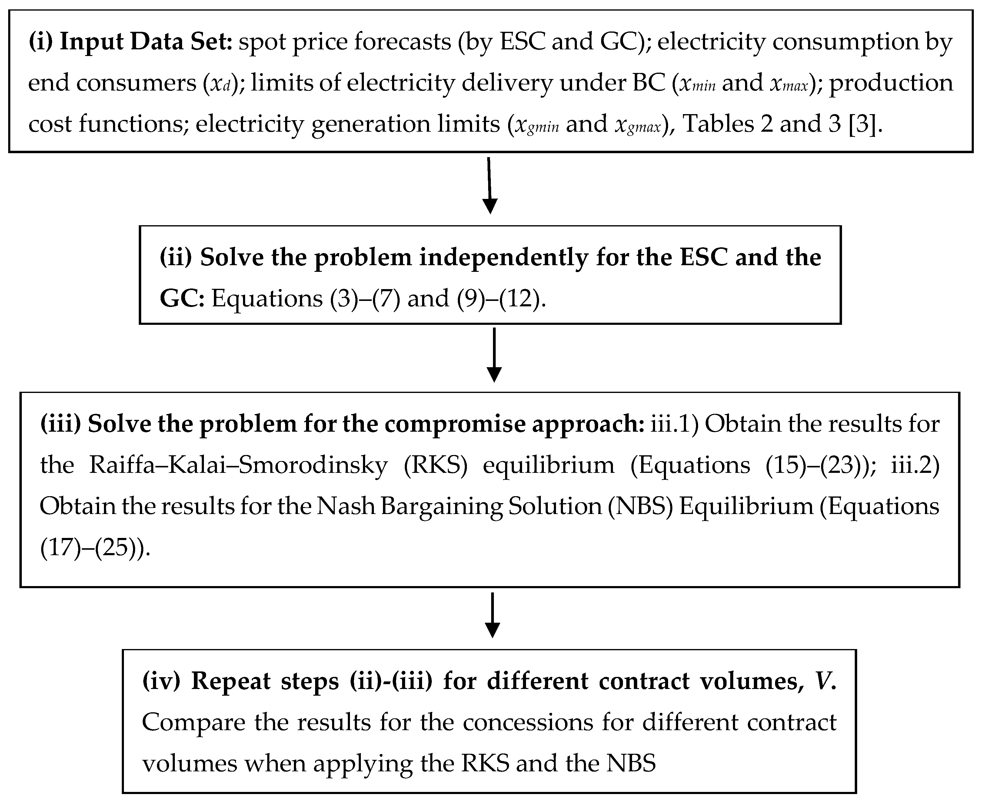
The concession of each player in the game, ESC and GC, have to be the same for both of them. The flowchart (i)–(iv) in
Figure 2 summarizes the implementation of the RKS bargaining solution.
4. Numerical Results for the RKS Compromise Approach
For the RKS compromise approach to work, it is necessary to consider that both the ESC and the GC, have independently scheduled their electricity deliveries in order to maximize their individual profits. The ESC should determine the electricity delivery scheduling by solving Equations (3)–(7). The data set used in this work by both the ESC and the GC is given in
Table 2 and
Table 3, respectively [
3]. Note that the spot price scenarios are not based on historical data, allowing us to compare the obtained results with the ones in [
3].
It is assumed that the contract periods consist of three equal time intervals. The amount of electricity to be delivered under the BC is
V = 145 MWh, and using the initial data in
Table 2, the results obtained by the ESC are presented in
Table 4. With independent scheduling, the ESC obtains a maximum revenue,
, equal to
$ 1807.9.
When the GC is doing the independent scheduling (similarly to contract type II), it must solve Equations (9)–(12). For a BC volume
V = 145 MWh, using the initial data in
Table 3, the scheduling proposed by the GC is shown in
Table 5. In that case, the GC has total expenses
that amount to
$ 1493.32.
The results obtained for the variables solving the compromise approach applying the RKS solution and the NBS are given in
Table 6. Note that the sum of the deliveries under the BC has to be equal to the total contract volume,
V = 145 MWh. As already stated, the results for RKS are obtained by solving Equations (15)–(23), while the results for NBS are obtained by Equations (17)–(25).
The revenue results obtained for the compromise approach are given in
Table 7, both for the RKS and the NBS equilibria. The results of NBS are replicated here, being the same as the ones obtained by [
3]. Furthermore, the negotiation region is larger when applying RKS instead of NBS.
When applying the RKS equilibrium, the ESC obtains higher revenues than when applying the NBS equilibrium, and the GC incurs in higher expenses when applying the RKS equilibrium than when applying NBS. It is quite an important point since the contract value obtained for the BC,
J, will be a little bit higher for the RKS case. The NBS results obtained are worse than the one applying the RKS approach. The values for the profits and for the relative concessions for ESC and GC are given in
Table 7.
When analyzing
Table 7, the profits, both for ESC and GC, are larger for the RKS approach. Moreover, the relative concessions for the ESC and the GC are lower when applying the RKS bargaining solution equilibrium. These relative concessions represent how much of the maximum profit any of the parties must give up to achieve the equilibrium. In particular, when the contract volume is
V = 145 MWh, the relative concession for the RKS bargaining solution is 55.01%, and the relative concession for the NBS is 56.08%, showing the best result obtained for the RKS approach.
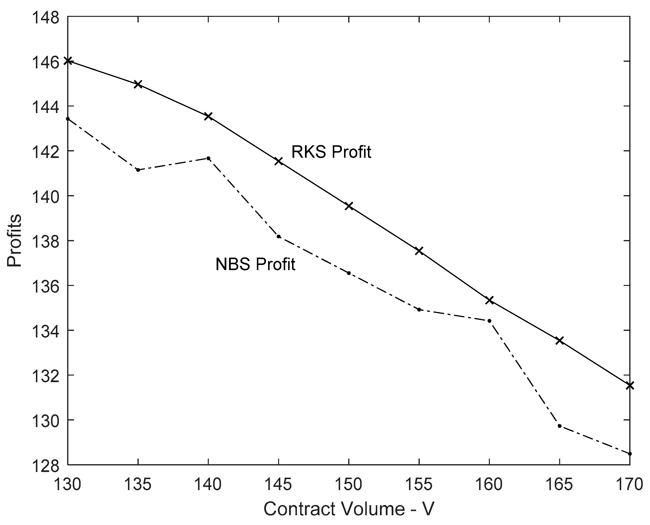
Finally, we have considered different values for the contract volume, where the contract volume varies, as shown in
Table 8. Moreover,
Figure 3 presents the same results for the varying profits when the contract volume is increased from
V = 130 to
V = 170. This research has considered increments of 5 MW in the contract volume, in order to show that even with these different contract volume values, the RKS bargaining solution approach obtains better results than the NBS equilibrium one.
As can be seen, the values obtained for the RKS equilibrium when varying the contract volume are always better than the results obtained for the Nash bargaining equilibrium. Quite interestingly, when the contract volume is above V = 165 MWh, the results obtained show the relative concessions to both parties to be lower than 50%. The lowest improvement when applying RKS and NBS is when V = 145 MWh.
Still analyzing
Table 8, there is a steady decrease in the concessions when increasing the contract volume from
V = 145 MWh. The best solution takes place when
V = 165 MWh; here, the solution of the RKS approach yields a total concession of 46.33% of its total profit, while, for the NBS, there is a total concession of 47.86% of its total profit. Furthermore, the largest difference when comparing RKS and NBS is 1.53% for
V = 165 MWh, whilst the lowest difference between the concessions for the two solutions, 0.33%, is for
V = 160 MWh. Finally, the profits for the parties, GC and ESC, are always higher applying the RKS approach when compared with NBS.
All the results presented have been obtained running the data set on a PC with one processor Intel Core i7 at 2.59 MHz with 16 Gb of RAM. The computations were done in Matlab, and the running time has been under one minute for each one of the cases presented.
5. Conclusions
This paper has proposed an RKS methodology to obtain the equilibrium of a BC used to hedge price volatility in the spot market and shortage risks. The results show that the RKS approach obtains better results than the NBS one. Also, when varying the value of the total contract volume from V = 130 MWh to V = 170 MWh, the RKS bargaining solutions obtained are better than the NBS ones being independent of the contract volumes.
For this particular problem, the worst results regarding the profit concessions are obtained when the contract volume is valued at 130 (
V = 130), being equal to 56.77% and 57.54% when applying the RKS and the NBS approaches, respectively. Moreover, the best results are obtained when
V = 165, is equal to 46.33% and 47.86% for the RKS and the NBS approaches, respectively. These results are quite important since, depending on the contract volume, a compromise approach can be achieved among the players without having to concede more than 50% of their maximum profits. The obtained results are also consistent with the fact that the RKS method provides lower concessions, providing better results in terms of profits for all. This is also supported by the findings of
Figure 3, where the RKS solution is always better than the NBS one.
In the future, improvements to the models, such as trying to analyze if the methods have just one equilibrium point, a special treatment for weekend data (calendar effect), and the inclusion of exogenous variables (water storage, weather, etc.) will be addressed. Furthermore, another possible extension will be to apply spot price forecasting models for the input spot price scenarios for the Electricity Supplier Company (ESC) and for the Generation Company (GC), making the model a more realistic one. Further research is required to better figure out how to apply the RKS equilibrium to problems where there is more than one player, including more than one ESC and more than one GC. Finally, we will consider the implications of the implemented RKS model in relation to the matching of producers and users taking part in the electricity market [
24].

 ,
, 


