1. Introduction
In recent years, the growth of distributed generation and residential prosumers [
1] has motivated energy companies to develop new ways of commercializing energy. Their main objective is to reduce the cost and improve the power system management. Accordingly, decentralized optimization processes that enable more participation of final customers expected to help this ambition [
2]. In order to facilitate higher cooperation of end customers (including both consumers and prosumers), intelligent decision-making systems are required [
3]. In the residential sector, these systems’ aim of minimizing the energy cost must also account for customers comfort. For instance, controllable loads, such as heating, ventilation, and air conditioning (HVAC), allow the cost reduction based on dynamic tariffs by taking into account preferable temperature set-points [
4].
The intelligent systems are considered as agents since they can perceive the environment and take decisions according to an objective [
5]. The quality of the decisions of an agent depends on the information that they have [
6]. Consequently, it is crucial to have reliable information about the environment. However, information can become unreliable due to shifting on weather conditions, integration of new devices, change of user preferences, and degradation of appliances.
Generally, for a residential prosumer agent, it is possible to distinguish two environments that are labeled as local and external. The former refers to the behind-the-meter resources [
7], while the latter describes situations where the prosumer agent can interact with other agents and information services. In most cases, the external environment only collects data of either weather variables or their forecast, but in a decentralized management scheme, it is possible to consider the external environment as a multi-agent system (MAS) [
8]. The agent is able to perceive the local environment by observing the power consumption data of different appliances. In fact, it constructs a time-series database by accumulating new information from a data stream [
9]. However, this process is problematic since agents have limitations on memory and processing time [
10]. In addition, the data stream can
drift over time, thus causing previously trained data models of appliances to lose accuracy [
11]. Therefore, model adaptation on the basis of recent data is essential [
12].
In this regard, several approaches have been developed to address the problems related to non-stationary data streams. In automated machine learning, active and adaptive learning algorithms have been utilized. The active learning techniques query for the information that they need each time for training a model [
13]. Beside, the adaptive learning methods only update the models when they detect a drift [
14]. Particularly, studies have considered retraining after fixed-size data windows and rule-based models as adaptation methods, applied to residential appliances models [
15,
16]. Therefore, they have underestimated the importance of drift issues on data management. Moreover, other researches have been conducted on training the models incrementally without analyzing the changes on data streams. For example, Farzan et al. increased the information of a transition matrix of a discrete-time Markov model to simulate both electricity and heating demands of individual households [
17]. Yoo et al. trained a Kalman filter, recursively, in order to forecast a household load, considering temperature and occupancy variables [
18]. However, adding the information of new samples directly to the models limits the set of models that can be used to represent the behavior of appliances. The applicability of these incremental learning techniques should be examined in detail according to the conditions of prosumer agents [
19].
Considering the above restrictions, the main objective of our study is to investigate adaptation methods that can be useful for prosumer agents to have more reliable information. Through extensive analysis, this paper contributes to:
The definition of the main criteria when choosing an adaptation algorithm in the context of prosumer agents. Here, the issues that the adaptation techniques address are examined to determine the best solution for models management, future concept assumptions, mixed drifts, and selection of training strategies.
The identification of suitable algorithms for adapting the prosumer agents models to overcome environment changes. The algorithms are estimated with different adaptation strategies and forgetting mechanisms, such as Adaptive Windowing (ADWIN) [
20], FISH [
21], and Drift Detection Method (DDM) [
22], in order to identify their required features in the prosumer agent context.
Proposition of a new adaptation algorithm based on triggered adaptation techniques and performance-based forgetting mechanisms. The proposed method is non-iterative; thus, it is less computationally complex than other methods in the literature. The suggested approach is capable of training several appliances’ models in relatively fast data streams for the prosumer agent context, using a single data window.
This paper is organized as follows:
Section 2 presents the problem of prosumer agents obtaining accurate information in a changing environment. The concept drift definition with the implications of the prosumer agent is also discussed in this section.
Section 3 explains the main criteria dictating the choice of a particular adaptation algorithm for the agents. Next,
Section 4 presents the proposed adaptation algorithm for prosumer agent models.
Section 5 presents the experimental setup and the comparison of results obtained by using different algorithms followed by the concluding remarks in
Section 6.
2. Problem Statement
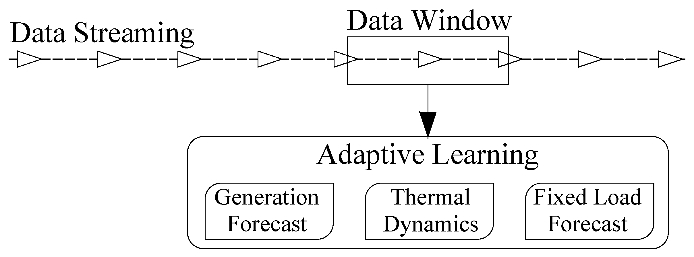
The local environment of the prosumer agent is composed of several appliances and local power generation systems. In order to reduce the number of variables, residential appliances are aggregated into two main groups, namely fixed loads and controllable loads. Controllable loads correspond to the appliances that can give some flexibility to the user, allowing him to modify energy consumption according to external signals he receives. Particularly, controllable loads that are examined in this study consist of heating systems because they are the most common flexibility source in the residential sector. In order to forecast both household power demand and know the thermal dynamics, the local environment is modeled with the data window that the agent creates from the data stream, as shown in
Figure 1. These models have been generally constructed based on supervised machine learning methods. [
23]. For fixed loads and local power generation, the models objective is only to forecast total power since the agent cannot take any action over these two elements. On the other hand, the model of controllable loads is developed to estimate the internal temperature based on the household power consumption profile, decided by the residential agent. As mentioned, this decision has to take into consideration the occupants’ comfort levels.
In all cases, residential prosumer agents need to adapt their models to new environmental conditions. An essential prerequisite to perform effective adaptations is to analyze the causes of data changes and the impacts of these changes on agents knowledge. In this context, it is important to notice that, for data-driven models, the underlying joint probability between features and targets is known as a concept, and it is assumed to be invariant over some interval of time. However, this underlying distribution could evolve over time sufficiently to cause a so-called concept drift [
11]. The formal definition of concept drift is presented in Equation (
1), where the
X stands for the input features (or observations),
y is the target variable (or label), and, hence,
is the joint distribution (or concept [
21]) evaluated at time
t and
.
Due to causality between the features and the target, it is suitable to consider the following form of the joint probability distribution [
24].
where
is the posterior probability of the target given the features, and
is the prior distribution of the features. For example, weather variables as features are subject to changes with seasonal conditions that are explained by the term
. Besides,
being the conditional distribution on features could also incorporate time-dependent effects, such as degradation of appliances.
As mentioned, the solution to deal with inaccuracy due to concept drift is to adapt the models parameters. However, before choosing an adaptation technique, it is meaningful to look at the characteristics of the concept drifts that can appear in the data streams of residential prosumers. Therefore, a prosumer-oriented study on the quantitative and qualitative measures of drift is provided below based on a general framework, discussed in Reference [
25].
2.1. Drift Magnitude
Drift Magnitude
measures the distance between two probability distributions at two different instants
t and
for
. Generally, drift magnitude is measured with the Hellinger distance
since it has a non-negative value, and the distance between A and B concepts is the same as B and A [
26]. However, it is possible to use other distance metrics, such as the total variation distance.
The drift magnitude can be used for drift classification. For example, a minor drift does not necessitate training the model. However, a major drift can imply the need for either retraining or changing the models (in case of ensemble learning mechanisms). In the data streams that a prosumer receives, it is possible to identify several minor drifts during the day at short timesteps that do not necessarily match with a gradual drift, especially for the fixed loads. Besides, when the time step goes bigger, the drift magnitude does not always increase, which means that there could be recurring concepts. For example, for the power generation model, if the prosumer has photovoltaic panels, the concept at dawn may be closer to the concept at night than at noon.
2.2. Drift Duration
The drift duration noted as m can define either a sudden (abrupt) or progressive (gradual or extended) transition between two concepts, depending on its value. As an example, in the local environment of a prosumer agent, a sudden concept drift (small drift duration) occurs when appliances are added, removed, or changed. Other special cases of concept transition like blip drifts and probabilistic drifts are hard to recognize by the prosumer since they can be mistaken for outliers in the data stream.
2.3. Drift Subject
Distinguishing a drift subject is difficult for prosumer agents since similar changes on features distribution can cause different drift subjects. However, it is important to mention that not all the drifts will require retraining the models. Normally, two categories of drift types are considered according to its causes [
25]:
Real concept drift: This type occurs when the posterior probability,
changes over time and requires a retraining of the model. The change can occur in either a portion of the domain of
X (sub-concept drift) or all of it (Full-concept drift).
Virtual concept drift: It happens when, instead, it is the distribution of the features
, which changes over time while the posterior probability,
remains the same. In that case, it is not always necessary to update the model.
2.4. Drift Predictability
The drift in a data stream can be related to independent events, such as seasons and days of the week. Consequently, it is possible to predict some aspects of the drift if the occurrence of these events is known. Furthermore, a concept drift can be predicted if a known recurrence pattern exists. Nevertheless, in the context of a prosumer agent, there can be different concept drifts coming from different environmental changes that cannot be well differentiated, so it will be barely impossible to anticipate the occurrence of certain types of drift. Moreover, define a magnitude threshold to identify the data that corresponds to previously seen concepts depends on the timestep that the prosumer agent uses.
3. Adaptive Algorithms
In this section, the adaptation algorithms are classified in order to identify suitable methods for residential prosumer agents problems. This classification is preceded by an examination of sub-issues that an adaptation algorithm faces [
21]:
The appearance of gradual drifts makes it impractical to assume that the concept of future data is always closer to the latest data. Therefore, instead of assuming the concept of future data, it will be useful to implement an algorithm that recognizes the distribution of the features of arriving data. Besides, in some applications of prosumers, the robustness of the methods is essential to differentiate outliers from concept drifts. However, in this study, the agent trusts the external information he receives from measurement systems and weather information services.
In the data stream, there could be different kinds of drifts mixed and outliers data samples. Another important concern with the concept drift in the specific context of the prosumer agent is the concurrence of the drift types. Thus the agent could be facing sudden drifts, gradual drifts, and incremental drifts within one timeframe [
27]. For that reason, adaptation algorithms that were made to solve problems related to specific cases of drift are not the best option for the agent. Here, we test some of those algorithms to validate this affirmation.
It is impractical for a prosumer agent to have different models trained with different data sets and ensemble the forecasts. Therefore, considering the available mechanisms to update the agents knowledge, when using a single model, the only strategy is to adapt the parameters. Nevertheless, in addition to parameters’ adaptation, it is also possible to combine the models by weighting them as in ensemble learning [
28]. The choice of the method should be made by taking into account the residential agent’s restrictions related to the processing time and hardware limitation. Normally, the models of three main groups are used to provide information for other processing systems, such as a Home Energy Management Systems (HEMS), with a practical objective, like either minimizing energy cost or maximizing comfort. These systems usually provide results in five to fifteen minutes intervals, thus limiting convenient exploitation of ensemble learning.
Not all adaptation techniques may work for all the models. The adaptation of parameters depends on the model type since some models can be trained incrementally, for example, by using adaptive linear neuron rule (ADALINE) or recursive least squares (RLS) [
29], while others have to start from zero every time. The drawback of incremental learning is that outliers are directly included in the model’s knowledge. Notwithstanding, it can reduce memory usage and processing time. Besides, the choice of the learning strategy depends on the nature of data and the rate of data collection. Thus, the residential agent could be receiving and processing the data under both forms of single or batch measurements. For instance, the labels of the models could be given every time while the features could be queried in batches each several hours.
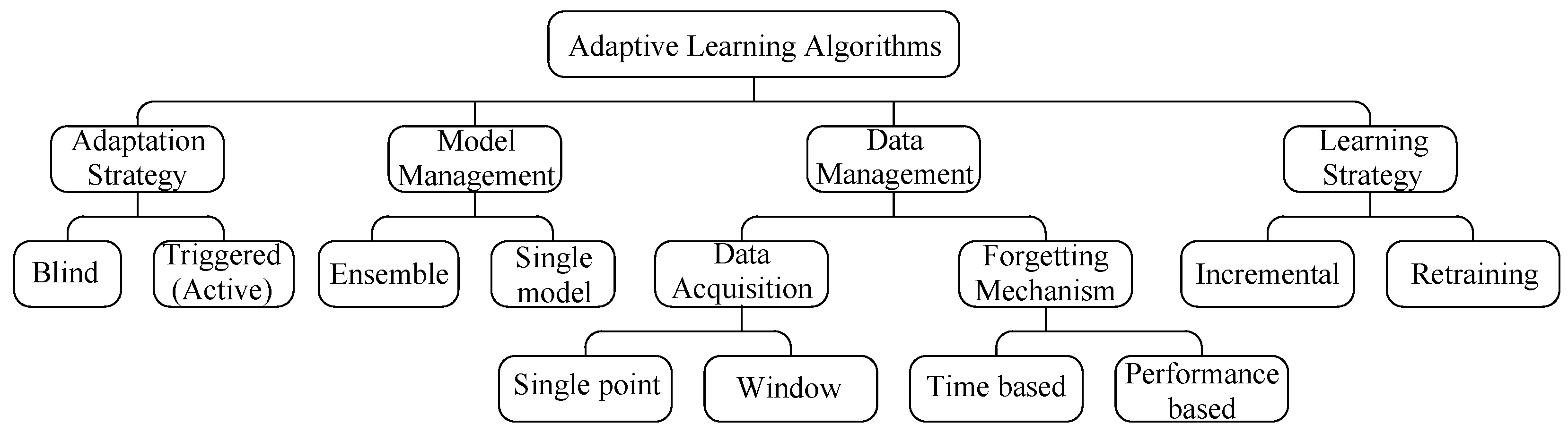
According to the above considerations, the taxonomy of adaptive learning algorithms is presented in
Figure 2. This classification is different from other ones, previously provided in Reference [
14,
30], due to the specificity of the prosumer agent. The new arrangement is to highlight the main concerns of agents over the choice of an algorithm, involving an adaptation strategy, model management, data acquisition, a forgetting mechanism, and a learning strategy. In
Figure 2, blind adaptation refers to a case in which the algorithm updates the model parameters at a pre-defined frequency without specific verification of the occurrence of concept drift in the data stream [
30]. Alternatively, some algorithms utilize a method to detect concept drift before triggering the adaptation. This mechanism is sometimes referred to as active adaptation.
The forgetting mechanism can be time-based in case the oldest samples are deleted, while the size of the data window either is kept fixed, changes according to a rule, or assigns fading factors to make old samples irrelevant. In addition, this mechanism can be performance-based in accordance with the adequacy of the samples for training the model or their similarity with future samples considering their statistical properties.
Now, with all the considerations for the prosumer agents’ problem, the following algorithms were selected to adapt the models of the local appliances. In addition, they present some remarkable characteristics that can be useful to formulate new methods.
3.1. Drift Detection Method
This method proposed in Reference [
22], starts with the premise that more items of the same concept in the data window will reduce prediction error. Consequently, it is possible to take an error increase as a proof of concept drifts [
31]. This is under the assumption that the base learner controls over-fitting.
For classifiers, the error can be modeled as a random variable from Bernoulli trials; then, the Binomial distribution gives the general form of the probability for the variable. In that context, if
is the error rate of the learner at time
t, then the standard deviation
will depend on the window size
as follows [
22]:
The algorithm storages the minimum value encountered of and the corresponding . Subsequently, two validations are made according to the confidence level:
Warning level: confidence level is 95%, so it is reached when .
Drift detection: confidence level is 99%, so it is reached when .
When the drift is detected, the onset of a new concept is declared starting at the time when the warning first appeared. As can be noted, this method was designed for sudden drifts. Hence, for residential agents, the algorithm will detect a drift several consecutive times when there are gradual drifts. For that reason, in order to apply this method, it was deemed necessary to define a minimum distance in time between a warning level and drift detection. Furthermore, the regressor models of the residential agent need to be considered as multi-label classifiers to implement this method. The method is summarized in Algorithm 1.
| Algorithm 1: Drift Detection method. |
![Energies 13 02250 i001]() |
3.2. Gold Ratio Method
This method proposed in Reference [
32] was also designed for adapting to sudden drifts. It assumes that the concept has changed if, at any time, the error of the model surpasses a defined level. The significance test must be sensitive enough to discover concept drift as soon as possible and robust to avoid mischaracterizing noise as concept changes. When the accuracy decreases, the oldest examples should be forgotten, and the size of the data window can be optimized by using a search algorithm in one dimension. The search algorithm used here is the Golden Ratio method. Considering a unimodal function, in the interval between a minimum window size (
) and the current size (
), the accuracy function has only one max at
. Then, the algorithm minimizes the number of function evaluations by dividing the range using the golden ratio
; in so doing, the optimal window size is clustered fast [
32].
The stopping criteria for the method is the minimum size of the search interval (100 samples proves to be adequate for the prosumer agent case). The significance test was done by using the root mean squared error (RMSE), and the acceptance level was adjusted according to the base learner. For the fixed load model, it is suitable to accept a higher RMSE since it is the most unpredictable signal. If no concept drift is detected, then the windows continue growing by adding more samples because a bigger training set will improve learning results if the concept is stable. The complete procedure is presented in Algorithm 2.
3.3. Klinkenberg and Joachims’ Algorithm
The idea of this method proposed in Reference [
33] is to select the window size to minimize the estimated generalization error. In the original case, the base learner is a support vector machine (SVM) because of the residual errors of the training
can give an upper bound of the leave-one-out errors without training the learner several times. However, the generalization error can still be minimized by using different window sizes and using k-fold cross-validation, assuming that most recent samples have a higher correlation with future features. In that way, this method can also be seen as a search method as presented in Algorithm 3.
| Algorithm 2: Gold ratio method. |
![Energies 13 02250 i002]() |
| Algorithm 3: Klinkenberg and Joachims’ Algorithm. |
![Energies 13 02250 i003]() |
3.4. Fish Method
For sudden concept drift, it should be possible to find the moment of the drift
by evaluating extensively for all the samples the likelihood between the distributions before and after that sample, using the Hotelling test, for example [
21].
However, when the drift is gradual, it is not only the distance in time which is relevant to select the samples needed to train the models. For that reason, the Fish method proposes to estimate also the distance in the feature space of the samples respect to the new ones [
21]. Thus, for each sample in the window, it will be necessary to calculate the combined distance [
34].
where
is the distance in time, and
is the distance in feature space of a sample in time
t with respect to the future features. Note that the existence of gradual drifts makes it necessary to give some relevance to the distance on feature space
. Subsequently, by organizing the samples according to their distance, it is easy to pick up the N closest samples to train the models. This method is best suited for the residential agents’ problems since it can account for both sudden and gradual drifts. The problem is to define a good distance function that gives reliable insights without increasing too much the processing time. The prosumer models have few features, so the feature space distance is calculated as the Euclidean distance because it is easy to compute and works well in low-dimensional spaces [
35]. The method is summarized in Algorithm 4.
| Algorithm 4: Fish method. |
![Energies 13 02250 i004]() |
3.5. ADWIN
This algorithm proposed in Reference [
20] is based on hypothesis testing. The idea is that, when two sub-windows have different averages
, the expected values are different. Like in a Hoeffding test, the null hypothesis is that the expected values are the same. The test can be written as follows for two different sub-windows of sizes
and
: If
, then the null hypothesis is false. Here,
corresponds to the average value of the sub-window, and
depends on the confidence value
according to:
For the problem of residential agents, analyzed in this paper, the confidence value is taken as 0.5%. The ADWIN method is summarized in Algorithm 5.
| Algorithm 5: ADWIN algorithm. |
![Energies 13 02250 i005]() |
4. Proposed Algorithm
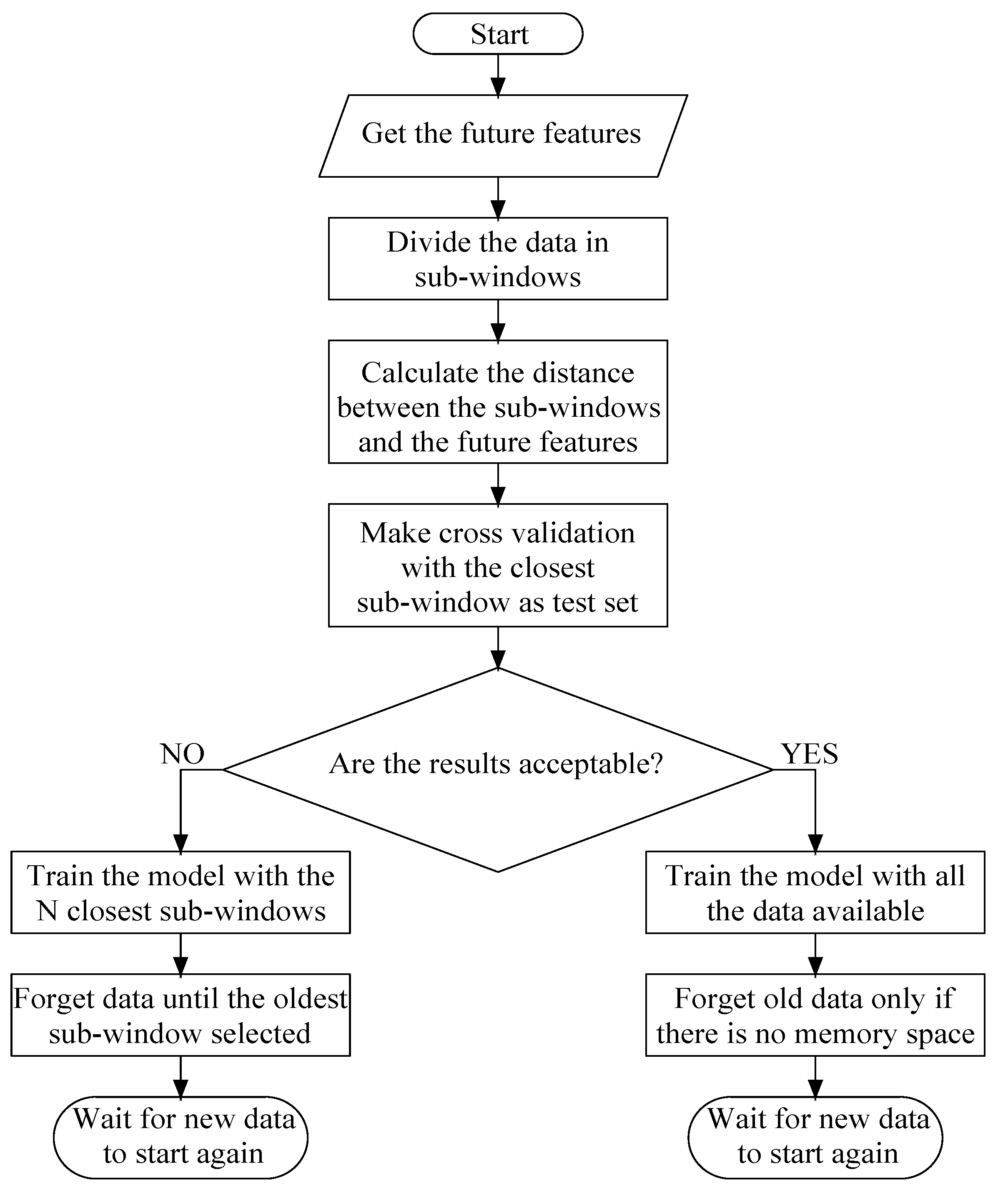
Given the collection of algorithms we presented above, we propose herein a hybrid approach that we think is best suited for the prosumer agents problem. Similar to the Drift Detection method and Gold Ratio method, the proposal is to use triggered adaptation. The algorithm will reduce the training set of the models only when the expected performance drops below a defined value, not each time that a new sample arrives.
To check the performance of the models, the procedure will be cross-validation using batches of the same size as the forecasting horizon (24 h, in this case), like in the Klinkenberg and Joachim’s method [
33]. The measurement of fit, in this case, is the RMSE because it gives more weight to bigger deviations; thus, it is better to identify the appearance of concept drifts [
36]. It is relevant to mention that the threshold to accept the results of the cross-validation depends on the nature of the target variable of each model [
37]. The test data set will be the closest batch to future features. Now, to identify that batch, the distance will be measured as in the FISH method [
34] as a combined distance in time and space of the samples. If the result of the cross-validation test is not good enough, then the model will be retrained only with the closest N batches. The parameter N needs to be tuned according to the model to avoid convergence problems in training but knowing that, when a concept drift appears, it is safer to train with a small amount of data to ensure that all samples correspond to the new concept.
Figure 3 summarizes the proposed algorithm with the procedure for when new data arrives.
Furthermore, forgetting data is a risky task since there are gradual drifts. The proposal here is to store a data window that contains the N selected samples, as well as the samples that were not selected but fall in between selected samples.
5. Numerical Results
In order to validate our proposal, we now report the results of a numerical experiment where we use a neural network as the power generation model, a decision tree for the fixed load, and a linear model for the thermal load. The details of the models implemented on Scikit-learn [
38] are shown here below:
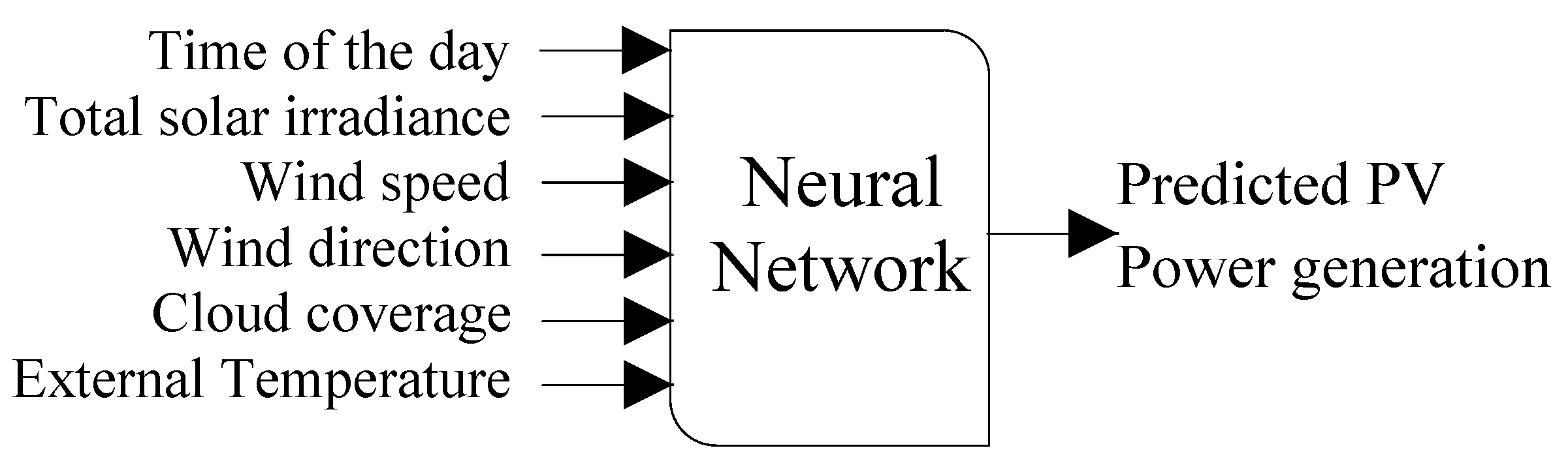
Power Generation: The base learner is a feed-forward neural network that forecasts the power output of a generation system
, as shown in
Figure 4. The hidden layers of the network have 100 × 5 neurons; the activation function is a hyperbolic tangent, the step size is fixed at 0.0001, the initial state of weights is 1, and the method used to train the model is stochastic gradient descent. The data used in this case was synthetically created by simulating a photovoltaic array in PVlib [
39] library with random cloud coverage (from 0 to 100% with transmittance offset of 0.75) and real temperature of Trois-Rivières, QC, in 2018.
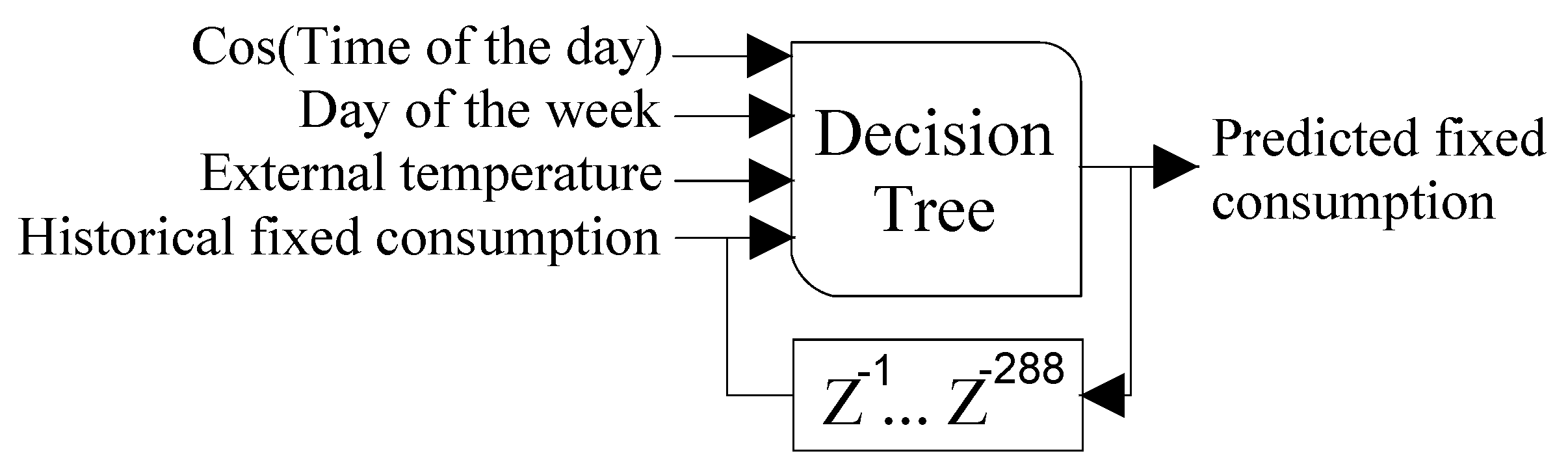
Fixed Load: The model to forecast the fixed load consumption
is a decision tree where the quality of a split is measured using the mean squared error, and nodes are expanded until all leaves are pure [
40]. The variables considered in this model are a cosine signal with a period of 24 h, the number of the day (from 1 to 7), the temperature, and the previous consumption (since the agent obtains data every 5 min, 288 samples correspond to 24 h). This model is presented in
Figure 5. The data used in this case is real measurements of the power demand of a house in Trois-rivières, QC, during 2018.
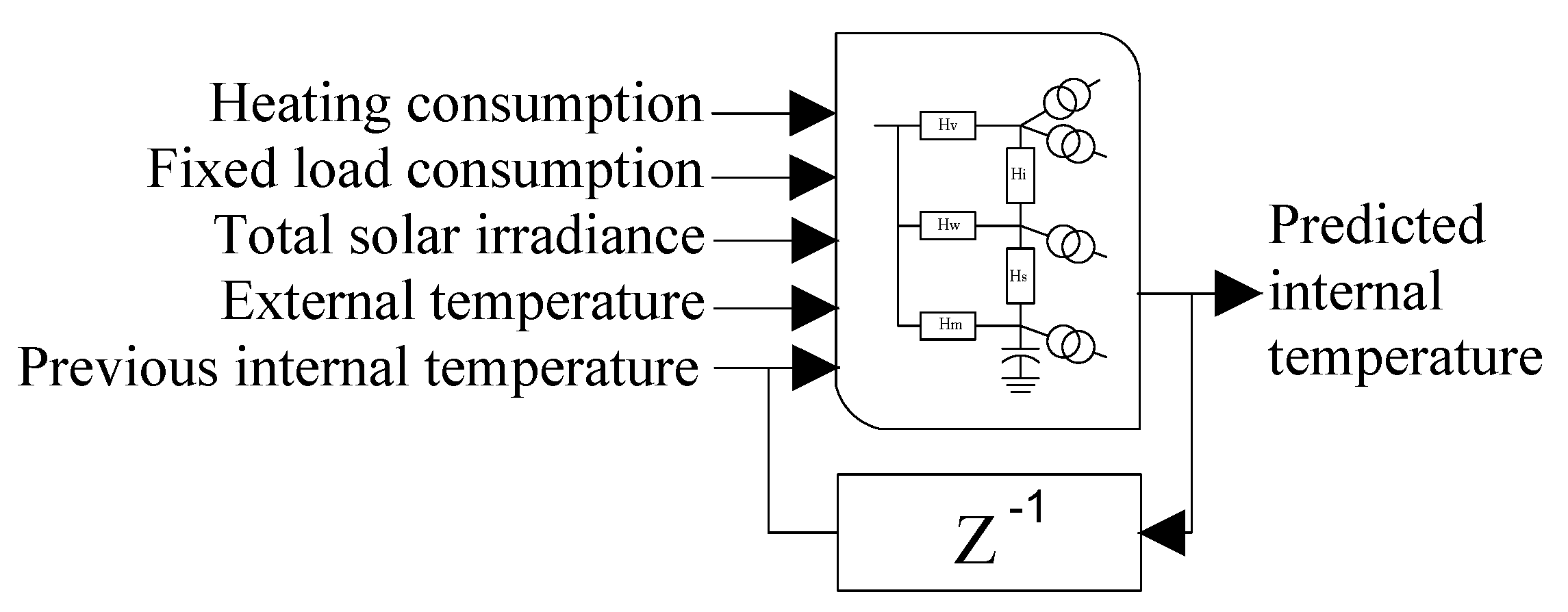
Controllable Load (Thermal model): This model s based on the equivalent circuit 5R1C proposed in the standard ISO 13790:2008 [
41]. The inputs in this case are the external temperature
, the fixed load consumption
, the solar irradiance
, and the power demand of the heating system
. The output will be the internal air temperature
. We assume that there is no special ventilation system, so there is only one external temperature as shown in
Figure 6.
The following equation describes the model.
where
corresponds to the internal temperature at timestep
. This linear model is trained by using Ordinary Least Squares (OLS) to find the parameters
,
,
,
, and
, which are combinations of the original parameters of the standard circuit model. The data used, in this case, corresponds to real measurements in a house in Trois-rivières, QC, during 2018.
The results presented here correspond to simulations starting in two different days when there are suspicions of concept drift: A spring day (19 April 2018) and a summer day (23 August 2018). As mentioned, when the concept changes, old data gives inappropriate data to the models, therefore the error is reduced by training only with the most recent data. In the selected days, there are symptoms of concept drift because when training the models with sliding windows, some times the smaller data window leads to lower errors. Training with sliding windows can be seen as a way to perform adaptation because, every time the agent receives new data, it retrains the models with the most recent data, adding the new samples and forgetting the oldest. Here, the training with sliding windows is used to detect possible concept drifts in data with the evolution of the RMSE. The normalized RMSE (RMSE) is obtained by dividing the RMSE into the range of the label signal.
The maximum limit of training data for each model is 8064 samples (28 days sampled every 5 min), and the minimum to ensure convergence is 2016 (7 days). The limits were established according to the models, the linear thermal model can be fitted with less than 2016 samples, but the power generation model does not converge with less than that. This information about the base learners is relevant since it is used to tune parameters of the adaptation methods. Here, the models started with previous knowledge (1 month of data) before beginning the adaptation. In the case that the agent does not have enough information, the parameters of the models can start with prior values [
42].
5.1. Spring Day
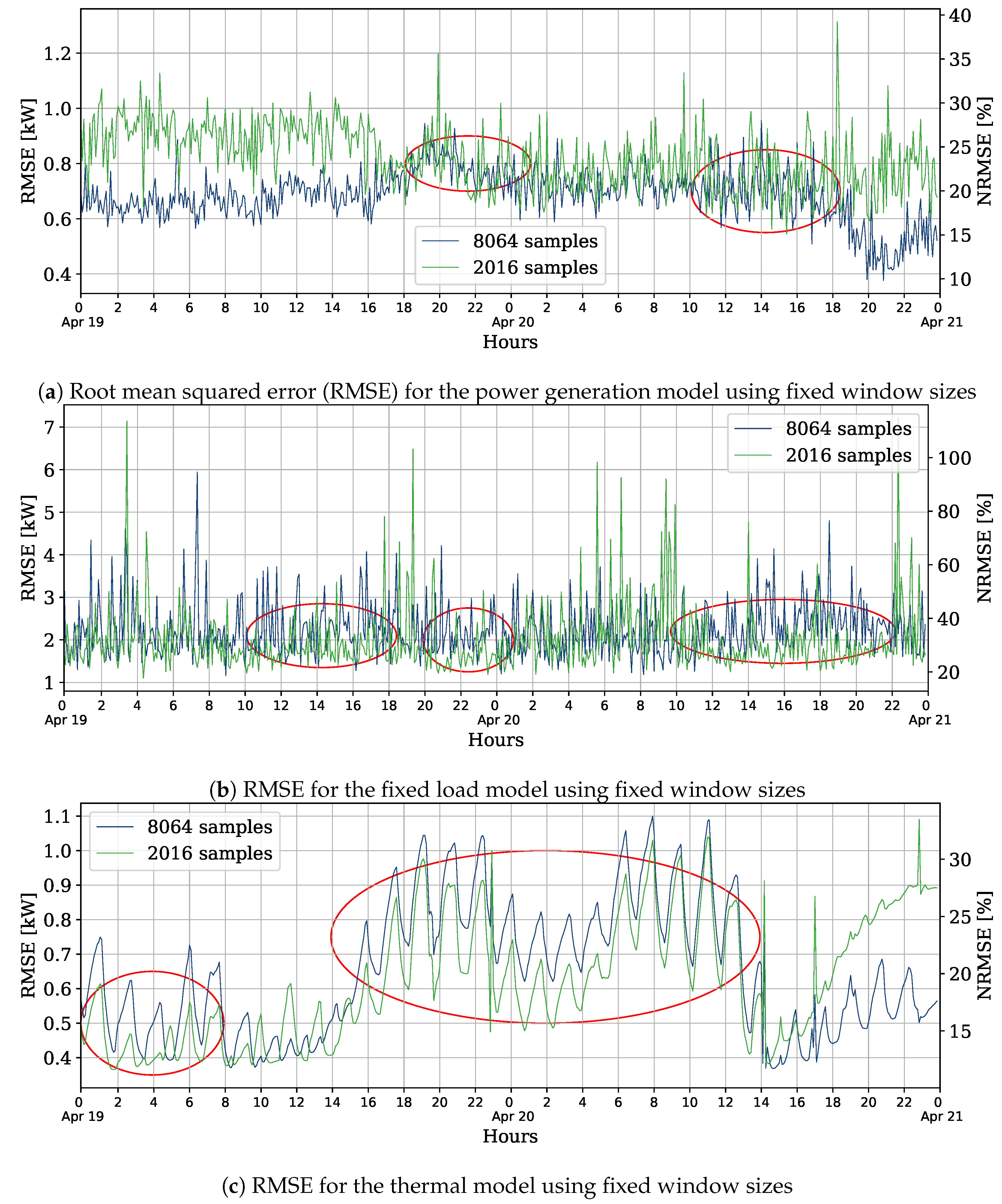
As can be seen in
Figure 7 with the evolution of the RMSE, running over 48 h, some periods seem to present concept drifts. For the power generation model, close to the 19 h of April 19th, it is possible to see an increase of the error when using a window of 8064 samples, that ends close to the 18 h of the next day. Similarly, for the thermal model, the biggest data window lead to a higher error most of the time, until the 14 h of April 20th. For these reasons, these days were chosen to test the adaptation techniques. On the other hand, for the fixed load forecast, the errors with both sizes of sliding windows are close most of the time, and some outliers on the label data may create prominent peaks.
Before presenting the results, it is pertinent to mention some characteristics of the the weather data on these days: the external temperature fluctuates in a range from 1.4 °C and 9.3 °C, with a mean of 6.06 °C; the maximum irradiation of 945 kJ/m2/h is reached at 12 h of the first day. The heating system of the house has a capacity of 15 kW, and the internal temperature goes from 17.6 °C to 21.1 °C, with an average of 19 °C.
Afterwards, the models were adapted during the selected period with the techniques presented earlier. The average RMSE (and NRMS) for each case is presented in
Table 1. The results obtained with the proposed method are systematically better than the most straightforward adaptation by sliding window, which means that implementing the method gives more reliable information to the prosumer than not doing so, even though the error reduction may be small. Other algorithms will occasionally perform better for adapting specific models. For example, the golden ratio method reduces the error when adapting the power generation model, but it is not suitable to adapt the thermal load model. Furthermore, the proposed method forgets less data, thus making it possible for the prosumer to use a single database for all three models.
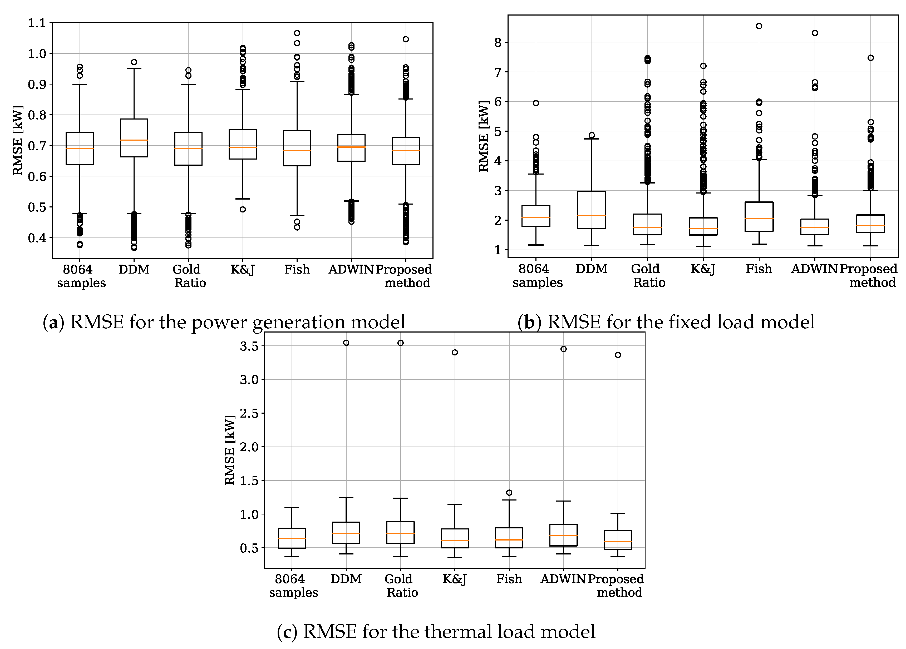
Another aspect that should be analyzed when choosing an algorithm is the dispersion of the error. Algorithms can be deluded by outliers and recurring concepts, leading to an increase in the error. Consequently, choosing a robust algorithm with low average error and low dispersion is important to give reliable information to the prosumer. In this regard, the performance of the proposed method is comparable with the others, as can be seen in
Figure 8. One compelling case is the FISH method to adapt the thermal model because it is less sensible than the all the other algorithms.
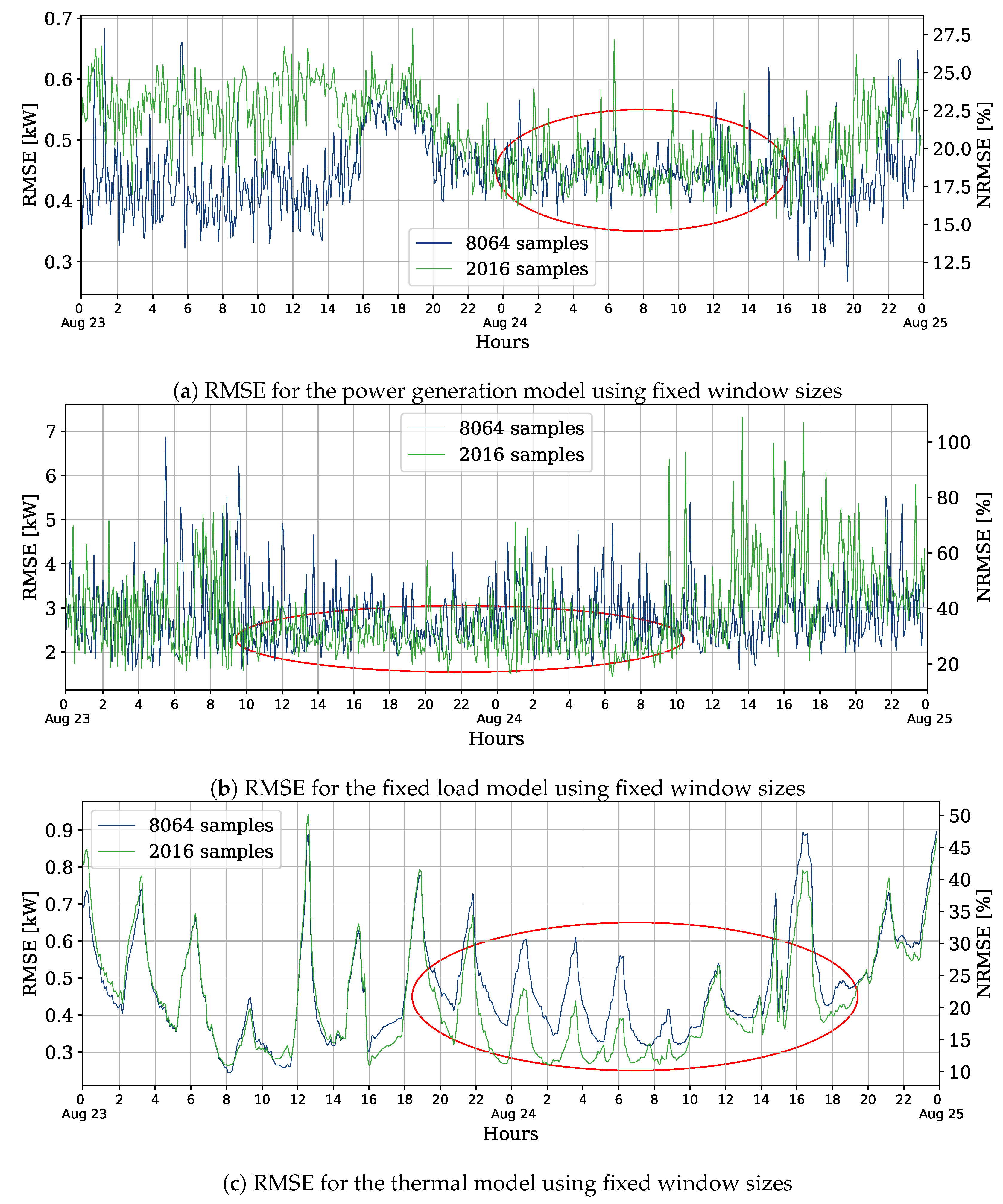
5.2. Summer Day
Similarly to the procedure to choose the spring day, we train the models using sliding windows to identify another day with signs of concept drift. On August 23rd, at 16 h, the error of the power generation model goes bigger when using 8064 samples than 2016, as shown in
Figure 9. For the thermal load, the error with the bigger data window also surpasses the other at the same time. Again, the results for the fixed load model are close, making it challenging to identify concept drifts. On these selected days, the external temperature has a range from 12.6 °C to 29 °C, with a mean of 22.4 °C; the maximum irradiation is 2900 kJ/m
2/h; and the internal temperature goes from 24 °C to 28.3 °C, with an average of 25.8 °C.
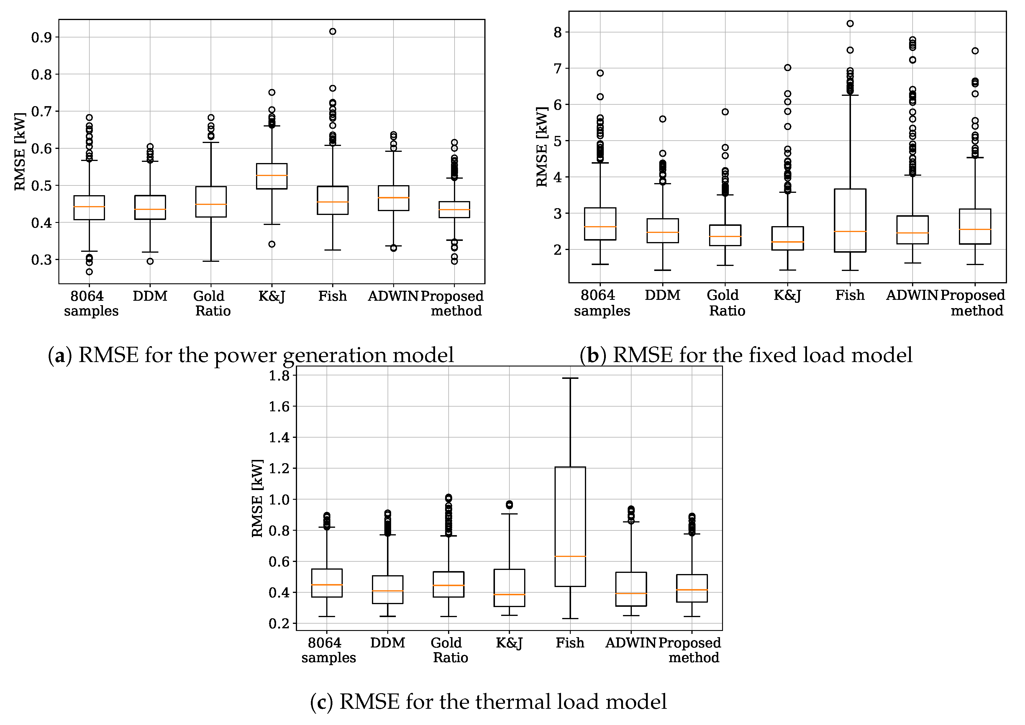
In
Table 2, the average RMSE for the selected summer days is displayed. Again, the proposed method performs better than the sliding window for all models. Nevertheless, for the fixed load model, the Klinkenberg and Joachims method achieves a lower average error. This result suggests that adapting different models with different techniques is preferable in some cases, even if that implies managing different databases for each model.
In this case, the dispersion of the error is comparable for all the methods, but, for the fixed load model, Drift Detection and Gold Ratio Methods seem to be less sensitive to outliers and recurrent concepts. On the other hand, in
Figure 10, it is shown that the FISH method has the biggest dispersion in all three models, which means it is not suitable for the kind of drift that appears on these days.
5.3. Results Analysis
As mentioned before, for the case of the prosumer agents, concept drift can appear in different ways, and they are hard to predict. As a consequence, forgetting data becomes a difficult decision because the agent could lose relevant information for the forecast. In this context, the proposal of keeping in memory more data than only the training set seems to be adequate for the agent. However, for some models, other methods obtain a better result using fewer data. For example, for the fixed load model, ADWIN and Klinkenberg’s methods had the lowest average errors. It is relevant to mention that these methods assume that future samples are more strongly related to the most recent data in memory, and it is not possible to keep that assumption when there are gradual drifts.
Another key finding of the experiment is in comparison with the average error when using a fixed data window. In particular, it is possible to observe that some adaptation techniques were not adequate since they lead to an increase in the error. In contrast, the proposed method always had a better performance than using a simple sliding data window. As for the parameters of the proposed algorithm, the error threshold for accepting the result of the cross-validation was 0.8 kW for the power generation model, 2 kW for the fixed load model, and 0.8 °C for the thermal model. For the parameter N, the used value was 2016 since it ensures convergence on the training of all the models in the tested periods. Tuning algorithms parameters depends on knowledge about the performance of the base learners, so the agents should have validated the models beforehand.
A final remark is that most of the algorithms have a fixed number of operations or training processes. The only method that has an indefinite amount of operations is the gold ratio search, for which the complexity is estimated at
(100 is the minimum search interval in this case) [
43]. Inevitably, this method takes more processing time than the others presented here. Since the models are trained with different amounts of samples every time, it is complicated to establish a metric to compare processing times.
6. Conclusions
Prosumer agents will play an essential role in energy management systems as they move towards decentralization. Then, it will be necessary to address their information needs to achieve adequate decisions. In particular, it is important to recognize that the agent environment is subject to change, and the models of different appliances need to be adapted to overcome different kinds of concept drift.
In order to formulate strategies to give the residential prosumers more reliable information upon which to base their decisions, this paper presented relevant criteria to account for when choosing adaptive algorithms to train the models of the local environment. Some of the existing algorithms in the literature were tested here with satisfactory results as they occasionally performed better than having a fixed window size.
Additionally, in this paper, we proposed another method that works for the information needs of the agents. The method depends on the number of batches selected to train the models; this parameter should be small to ensure that most of the samples correspond to the new concept but big enough to ensure the convergence when training the model. In experimental results, this algorithm was the only one that systematically produced better results than that obtained with a fixed data window size.

 ,
, 


