Assessing and Comparing Short Term Load Forecasting Performance

Abstract

When identifying and comparing forecasting models, there may be a risk that poorly selected criteria could lead to wrong conclusions. Thus, it is important to know how sensitive the results are to the selection of criteria. This contribution aims to study the sensitivity of the identification and comparison results to the choice of criteria. It compares typically applied criteria for tuning and performance assessment of load forecasting methods with estimated costs caused by the forecasting errors. The focus is on short-term forecasting of the loads of energy systems. The estimated costs comprise electricity market costs and network costs. We estimate the electricity market costs by assuming that the forecasting errors cause balancing errors and consequently balancing costs to the market actors. The forecasting errors cause network costs by overloading network components thus increasing losses and reducing the component lifetime or alternatively increase operational margins to avoid those overloads. The lifetime loss of insulators, and thus also the components, is caused by heating according to the law of Arrhenius. We also study consumer costs. The results support the assumption that there is a need to develop and use additional and case-specific performance criteria for electricity load forecasting.

1. Introduction

Bessa et al. [1] discussed two different ways of measuring the performance of a forecast. One way is to measure the correspondence between forecasts and observations (forecast quality). Another way is to measure the incremental benefits (economic/or other) when employed by users as an input into their decision-making processes (forecast value). Assessing forecast quality is more straightforward and the standard approach is statistical error metrics, such as:

• Mean absolute error (MAE),
• Mean absolute percentage error (MAPE), and
• Root mean squared error (RMSE).

Typically, these metrics apply some kind of loss function to individual errors and then calculate a summary statistic [2]. For example, Screck et al. [3] surveyed the literature for 681 load forecasts for the residential sector. Altogether, 15 error metrics were used, the most frequently used was mean absolute percentage error (MAPE) with 392 values. The second was normalized root mean squared error (NRMSE) with 209 error values and the third was RMSE. MAPE and NRMSE are relative metrics that aim to be comparable amongst different experiments. In the literature, the meaning of NRMSE varies significantly, because there are many different ways to normalize the RMSE. Here, we use only the most common definition that normalizes RMSE by dividing it by the mean of the measured values. In the alternative definitions, the normalization is done by the difference between the maximum and minimum, by the standard deviation, or be the interquartile range, etc. Some publications, such as [4], even use a NRMSE definition that, similarly to MAPE, normalizes each individual error with the simultaneous measured value before calculating the RMSE. So defined NRMSE and MAPE are much more sensitive than the NRMSE we use to calculate absolute errors when the actual loads are small or very small. MAPE also puts less weight on large deviations than NRMSE. MAPE is based on assumptions that (1) accurate forecasting of small loads is important and (2) one large error is not more significant than an equally large sum of small absolute errors. Both these assumptions are clearly in conflict with the actual consequences of the short-term load forecasting errors that we discuss next.

Often, model identification is easier and computationally more efficient with quadratic criteria such as sum of squared errors (SSE), RMSE and NRMSE. These criteria also reflect the combination of errors from several independent sources. This is important, as typically several different component forecasts are needed for forecasting the total power or power balance. The assumption of independence may not be completely valid, however. For example, the forecasts of loads and generation are often based on the same or mutually correlated weather forecasts or are connected by the behavior of certain groups of humans. Technologies and energy markets also reduce independence of load behavior. For example, demand side responses for electricity markets and ancillary services have very much mutual correlation. Good short-term load forecasting methods utilize such dependencies efficiently and their forecasting errors tend to be rather independent from each other. Correlated forecasting errors may also stem from using the same forecasting methods or methods that have common weaknesses. Mutual correlation of forecasting errors is usually easy to detect, and it is a sign that improving the forecast is possible.

The concept of forecast value, on the other hand, views the forecast user’s business process more extensively and is more difficult to assess. Forecast value includes the economic and noneconomic benefits which are available to the user by using the forecast. An example is the reduction in imbalance costs for a balance responsible party. A crucial aspect is that the value is user and problem specific [1]. For example, power market participants and the system operator may measure forecast value differently. For the system operator, the most important issue is the expected maximum forecast error, and not the mean forecast error. An UCTE position paper [5] discussed this issue for wind power forecasts. We will employ a case study below to explore to what extent the consumer and the retailer aggregator have different preferences. Such differences between different actors largely stem from the fact that the electricity markets locally and imperfectly approximate marginal cost changes, but do not perfectly reflect the real costs of the power systems.

It is often infeasible to calculate the benefits of the forecast accurately. When it is possible to accurately model the decision-making process which exploits the forecasts and the resulting costs, the error metric can be selected so that the resulting costs are minimized [6].

Forecast value is also related to the error metrics. According to [6], error metrics should be easy to interpret, quick to compute and reflect the net increase in costs resulting from decisions made based on incorrect forecasts. MAPE also penalizes over-forecasts (where forecast load is greater than realized load) more than under–forecasts [7,8]. In addition, MAPE penalizes relatively lightly such large absolute forecasting errors that occur during load peaks. However, in short-term load forecasting, under–forecasting high loads tends to be especially costly for all the relevant actors, including the system operator and the energy consumer.

The most commonly used error metrics also suffer from a double penalty effect for events which are correctly predicted but temporally displaced [7,9]. There are criteria, such as the parameterized earth mover’s distance [10], which do not suffer from this effect. For avoiding this double penalty effect, time shifted error measures such as dynamic time warping and permutated (so called adjusted) errors and their downsides are considered by [9].

Costs of large mutually correlated forecasting errors may behave differently from the SSE and RMSE. MAE assumes that the costs due to forecasting errors depend linearly on the size of the errors. It is often used to avoid the problem that SSE and RMSE put too much weight on large forecasting errors as compared to the assumed real costs. Often this assumption is not valid and the actual costs may grow even faster than the square of the error assumed in SSE and RMSE.

The power systems are changing in an increasing speed. Distributed new energy resources such as active loads and other controllable distributed flexible energy resources make the power flows in distribution grids more variable than before. The power flows to and from the customers of the grid are correlated due to control actions, solar radiation and wind. The traditional load forecasting methods become obsolete. The forecasting performance criteria also need some reconsideration and updating in order to fit to this new situation.

Our aim in the present work is to show that there is still a need to develop the understanding, selection and amendment of criteria for forecasting performance. In forecasting applications, assessing or measuring the incremental benefits from the forecasts is both necessary and difficult. With case studies, we assess how the forecasting errors increase the costs of the competitive electricity market actors, electricity network operators and their customers, the consumers and prosumers that use the power system.

2. Needs to Develop Short Term Load Forecasting Criteria

When studying and developing short term load forecasting methods for active demand, such as [11], we have detected the following challenges:

• Assessing the economic costs of forecasting errors on the electricity markets is more complex than often assumed.
• The cost impacts tend to be asymmetric. Under-forecasting the load peaks typically causes higher costs than a similar amount of over-forecasting.
• The economic costs of forecasting errors tend to concentrate to the load peaks at the network bottleneck and system levels and to the rarely occurring high price peaks on the markets for electricity and the ancillary services of the power system and grids.
• Some popular and useful methods tend to predict higher and shorter load peaks than what actually occur.

The costs of forecasting errors to the competitive electricity market actors mainly stem from the balancing errors caused to their balance responsible party. When forecasting only components of the total balance, the errors relative to the errors in the total balance matter and the errors relative to the component forecast itself are not at all relevant. In addition, we need accurate forecasting during the system peak loads and peak prices and the highest peaks are rare and unpredictable.

Underestimating the load when forecasting critical high load situations can lead to very expensive unwanted measures in managing the grid constraints or peak load reserves at short notice.

A common problem with black box methods, such as machine learning methods, is that although they generally tend to under-forecast load peaks, as shown in [4], for rarely occurring outdoor temperature related peak loads they tend to predict higher and shorter load peaks than what actually occur. This tends to happen because (1) the identification data do not include enough such extreme situations in order to model the load saturation effects or (2) many nonlinear black box methods tend to have large errors when extrapolating outside the situations included in the identification data. There are several methods to deal with this problem. Daizong Dint et al. [12] proposed using (1) a memory network technique to store historical patterns of extreme events for future reference and (2) a new classification loss function called extreme value loss (EVL) for detecting extreme events in the future. Those approaches can improve the deep neural network (DNN) performance regarding only those extreme events that have been included in the learning data. Another approach is to add another model for the power range and use that for limiting out those forecast values that exceed the limit by more than a tolerance [4]. Then, the energy of the peak should be preserved by extending the length of the peak. Physically based model structures describing the existence of constrained maximum power are useful for such peak limitation. Physically based model structures with power constraints can also be used to model the main phenomenon that contributes to the peak load. We have improved forecasting of rarely occurring and extreme situations by combining several different models into hybrid models, see [11] for an example. In order to better assess, compare and develop methods, we need forecasting criteria that adequately reflect the concentration of the economic costs of the forecasting errors to the high load situations.

3. Cases Studied

3.1. Electricity Market Costs Due to Forecasting Errors

The costs relate to the overall forecasting error of the total energy balance of the balance responsible party of the actor in the market. Thus, the load forecast of a consumer group segment is only one component of the total forecast. There are forecasts for different types of load and local generation. The different forecasts are not fully independent, because many of them may use the same weather forecasts and be subject to interactions between consumer group behavior. However, the errors of accurate forecasters tend to be independent and it is easy to check to what extent this assumption holds. Going to such details is complicated and outside the scope of this paper. Thus, for clarity of the analysis, we assume that the errors of different segment forecasts are independent. Then the contribution of the expected individual error component e₁ to the total expected forecast error e is as follows.

$$\mathrm{E}\left[e^2\right]=\mathrm{E}[e_0{}^2+e_1{}^2\left]=\mathrm{E}[e_0{}^2\right]+\mathrm{E}[e_1{}^2]$$

(1)

where e₀ is the expected total error of all the other forecast components. Figure 1a shows how the total error e behaves as a function of e₁ when e₀ is set to 1. For small e₁, the increase in e is quadratic.

The monetary cost of the total forecasting error needs to be assessed in the electricity market. For simplicity, we assume that the forecasting errors cause costs via the market balancing errors. The market rules for penalizing the balancing errors of loads vary from country to country. The Nordic power market applies the balancing market price as the cost of the balancing errors. In the Nordic countries, one price system is applied for errors in consumption (load) balance and, in addition, there is a small cost component proportional to the absolute balancing error (volume fee for imbalance power). Power generation plants below 1 MVA are included in the consumption balance.

The price of consumption imbalance power is the price for which Fingrid both purchases balance power from a balance responsible party and sells it to one. In the case of the regulating hour, the regulation price is used. If no regulation has been made, the Elspot FIN price is used as the purchase and selling price of consumption imbalance power. For an explanation, see [13]. All the prices and fees are publicly available at the webpages of Fingrid and NordPool, such as [14]. In addition, imbalance power in the consumption balance is subject to a volume fee. There is also a fee for actual consumption, but that depends only on the actual consumption and not on the forecasting errors. The volume fee of imbalance power for consumption during the whole study period was 0.5 €/MWh. See [15] for the fees.

From an actual or simulated component load forecasting error, the resulting increase the forecasting error of the total energy balance can be calculated, and using this increase in error the resulting balancing cost increase was calculated based on the price of imbalance power and the volume fee of the power imbalance. In this way, we got an estimate for how much electricity market costs the forecasting error causes to the balance responsible actor. We do not know the forecasting errors of the balance responsible party. In the following study, we generated them as a normally distributed sequence that has standard deviation 3 MW. The actual errors may be bigger, but as we see later, that will not affect the conclusions. The price of imbalance price occasionally has very high peaks. Thus, the cost estimate will be very inaccurate, even when a very long simulation period is applied. It is necessary to check the contribution of the very highest price peaks to the cost in order to have a rough idea on the inaccuracy of the results. We avoided this challenge as follows. We made a short-term load forecast using a residual hybrid of physically based load control response models and a stacked booster network as explained in [16] for a four-year-long test period. We found out that the forecasting errors were rather well normally distributed and bounded. We generated 200 random normally distributed bounded error sequences over the four–year period. With each one of these 200 normally distributed bounded random error sequences, we calculated the balancing error costs for the forecast group. Then, the standard deviation of the group errors was varied and the same cost calculation repeated. The variation of the costs between the error sequences was very large. The mean behaved as assumed in Figure 1a and an actual measured and forecast case was clearly in the area where the quadratic dependency dominates (see Figure 1b). The demand response aggregator considers the actual and forecast active loads as trade secrets and does not allow us to make them public information. Except for this one point, all data used for the simulations in Figure 1 are publicly available.

The balancing error cost was very stochastic, because the impact of high balancing market price peaks dominated (see Figure 1c). The balancing error cost over the whole four-year-long period mostly depended on the forecasting error during those few price peaks. The red circle represents the forecasting errors when an experimental short-term demand response forecasting algorithm was applied to the forecasting on the morning of the previous day. There, the aggregated controllable power was slightly over 18 MW. The results support the use of the quadratic error criteria std. and RMSE, rather than linear criteria such as MAPE etc. In this case, data driven forecasters that do not model the dynamic load control responses have so poor accuracy that the cost dependency approaches a linear dependency. Here, we have ignored the fact that especially large forecasting errors can affect the price of imbalance power significantly, thus increasing the balancing error cost much more than linearly.

Another observation is that with the good performance forecasting model, the forecasting errors increased the imbalance costs very little, only 0.53 € per controllable house annually. This suggests that the one price balancing error model gives only very weak incentives to improve the forecasting accuracy in normal situations. The one–price balance error cost model may not adequately reflect the situation from the power system point of view. A further study is needed to find out to what extent, how much and with which market mechanisms the power system can in the future benefit from improving the short-term forecasting accuracy. A conclusion of the H2020 SmartNet project [17] was that improving the forecasting accuracy is critical for getting the benefits from the future ancillary service market architectures for enabling the provision of the ancillary services using distributed flexible energy resources.

Some other countries apply a two–price system for balancing error costs. That means that the price for the balancing errors is separately defined by the balancing market for both directions. Then the costs of load forecasting errors are much higher than in a one–price system. They may even exaggerate the related needs of power system, if the errors of the forecasts of the individual balancing are assumed to be independent from each other. When the share of distributed generation increases, the one price system may become problematic, because the consumption and distributed generation may not have enough incentives to minimize their balancing errors. This increases the need for balancing reserves in the system. The share of distributed generation is expected to increase much during the summertime, which means that also in the Nordic countries there may appear needs to change the market rules regarding the balancing costs somehow. Moving to two–price system may be one such possibility. Thus, it may be worthwhile to repeat the above study using the two–price system of the generation balance.

3.2. Distribution Network Costs Due to Forecasting Errors

Overloading of network components causes high losses that increase the temperature of the components. Overheating reduces the lifetime of the insulator materials in the network components rapidly. If the forecast underestimates the peak load, the operational measures to limit overload are not activated in time, energy losses increase and the component aging increases so much that the expected lifetime is reduced.

The losses in the network components are generally proportional to the square of the current. When the voltage is kept roughly constant and the reactive power, voltage unbalance and distortion are assumed to be negligible, the losses are roughly proportional to the square of the transferred power. In real networks, these assumptions are not accurate enough. Strbac et al. [18] calculated losses using a complete model of three power distribution license areas in UK. The analysis highlighted that 36–47% of the losses are in low voltage (LV) networks, 9–13% are associated with distribution transformer load related losses, 7–10% are distribution transformer no-load losses and the remaining part in higher voltage levels. They [18] (p. 43) showed the marginal transmission losses as a function of system loading. A 1 MWh reduction in load would reduce transmission losses by 0.11 MWh during peak load condition (100%). When system loading is 60%, reducing the load by 1 MWh will reduce transmission losses by 0.024 MWh. This corresponds to the dependency f(P) = P^2.98. The sample size is small, so the accuracy of this dependency is questionable. Nevertheless, the dependency is clearly different from f(P) = P² that results from assuming constant voltage at the purely active power load and transmission losses relative to the square of the current. Underestimating the peak loads causes much higher losses and related costs than other load forecasting errors. Thus, the impact of forecasting errors to the energy losses is very nonlinear and depends on the direction of the error and size of the load.

Ref. [19] studied how transformer oil lifetime depends on temperature. Arrhenius’ law describes the observed aging rather well. Aging mechanisms of cable polymers were discussed in [20]. The Arrhenius method is often used to predict the aging of cable insulation, although it is valid only in a narrow temperature range. For example, it is applicable only below the melting point of the insulator. For simplicity, we here model the aging using the Arrhenius method. According to it, k the rate of chemical reaction (such as insulator aging) is an exponential function of the inverse of the absolute temperature T.

$$k=\mathrm{A}{e}^{-{\mathrm{E}}_{\mathrm{a}}/\mathrm{R}T}$$

(2)

where R is the gas constant, and the pre-exponential factor A and the activation energy E_a are almost independent from the temperature T. In the steady state, the difference between the component or insulator temperature and the ambient temperature is linearly proportional to the losses. Components are normally operated much below their nominal or design capacity and the impact of forecasting errors on the losses and aging is small. When the component during peak load is operated at or above its nominal load and is subject to high ambient temperature and poor power quality high losses, fast component aging, or expensive operational measures result from under-forecasting the load.

Thus, the impact of forecasting errors to the costs is very nonlinear and depends on the direction of the error and size of the load. Most of the time, the network costs from short term load forecasting errors are small or even insignificant. However, the costs of forecasting errors increase rapidly when the load is at or above the nominal capacity of the network bottlenecks, if the actual load is higher than the forecast load.

3.3. A Consumer Cost Case Study: Load Forecasting Based Control of Domestic Energy Storage System

All the costs of the power supply are paid by the users of the electricity grid. The forecasting errors discussed in the other chapters increase the electricity prices and grid tariffs by increasing the costs of the electricity retailers, the aggregators and the grid operators. Here, we consider those costs that the consumer has possibilities to control more directly.

By using energy storage in a domestic building, a customer can get savings in the electricity bill [21]. The amount of the savings depends on many factors. The load profile of the customer and the electricity pricing structure and price levels are the main variables that affect the savings, but the customer has very limited possibilities to change them. The size of the energy storage can be optimized for the customer’s load profile, but after that, controlling the energy storage and consumption is the only way to maximize the savings. Energy storage can be used, e.g., to increase the self-consumption of small-scale photovoltaic production, but it can also be used for minimizing costs from different electricity pricing components. If the energy retailer’s price is based on the market price of electricity, the customer can get savings by charging the energy storage during low price and discharging during high price as in [21]. If electricity distribution price is based on the maximum peak powers, the customer can get savings by discharging the battery during peak hours, as in [22].

Such electrical energy storage systems are still rare and typically installed to increase the self-consumption of small-scale photovoltaic power production. Although the battery technologies progress all the time, the profitability in such use is still typically poor, especially if there are loads that can be easily shifted in time. One can improve the profitability of the battery system significantly by having several control targets or a more holistic one. Such a possibility is minimizing the costs from different electricity pricing components, but that requires short–term load forecasting.

In this case study, it is assumed that every customer in the study group has a market price-based contract with an electricity retailer and the distribution price is partly based on the maximum peak powers as in [23]. The energy retailer price is based on hourly day-ahead market prices of Finland’s area in Nord Pool electricity markets [13]. The electricity retailer adds a margin of 0.25 c/kwh to the hourly prices. Distribution prices are based on the study in [23], where the price components were calculated for the area of the same distribution system operator (DSO) as where the customers’ data of this study were measured. The price structure includes two consumption-based components: volumetric charge (0.58 c/kWh) and power charge (5.83 €/kW). The power charge is based on the monthly highest hourly average peak power. When value added tax (24%) is added to these charges, the prices which affect to customers’ costs are: volumetric charge 0.72 c/kWh and power charge: 7.23 €/kWh. The same prices were used in [22].

Customers’ load data are from one Finnish DSO, whose license area is partly rural and partly small towns. The study group consists of 500 random customers. In simulations, each customer has 6 kWh with a 0.7 C-rate Lithium-ion battery. Battery type is lithium iron phosphate (LFP), because it has good safety for domestic use. The energy storage system is controlled firstly to decrease the monthly maximum peak power and secondly to decrease the electricity costs with market price-based control as in [22]. The battery is discharged when power is forecast to increase over the monthly peak and charged during low prices. The market price-based control algorithm and battery simulation model were presented in [21]. In previous studies, the controlling of energy storage was based on load forecasting. The load forecasts are based on a model, which utilizes customer’s historical load data and temperature dependence of load with temperature forecast [24].

In the present study, the dependence between the accuracy of load forecasting and the customers’ savings achieved by using the energy storage are studied. The simulations are made for every customer with 11 different load forecasts each having a different load forecasting accuracy. The forecasting accuracy is varied by scaling the forecast error time series. The actual load forecast time series is nominated as the basic level (100%) and the real load data correspond to the ideal forecast (0%). The range of studied error scaling is selected linearly between 0% and 200%, with 20% step size in every hour. Customers’ yearly cost savings and different forecast accuracy criteria (SSE, RMSE, NRMSE, MAE and MAPE) have been calculated during simulations. Additionally, because most of the savings come from the decrease in monthly peak powers, the MAE of monthly peak powers (MAE_max) was calculated. The monetary value of the cost savings depends on the customer’s load profile, so the results are given as percentage values of cost savings. The results of the simulations are shown in Figure 2. From the result points, we calculated least-squares fitted line (R1) and least-squares fitted second-order curve (R2).

From the results, we see that with ideal forecasts the savings of the customers vary a lot. This stems from the different load profiles of the customers. The customers, whose load profile includes high peaks during several months, can get very high savings. If customer’s load profile is very flat, the savings can be low. When the errors in the forecast start to increase, the savings drop very fast at first, but the decrease in the savings slows quickly and the decrease stays low until the end.

From the results of Figure 2 and the results of least-squared fittings, we collected the main results and values for the

Table 1. Comparison of criteria in a consumer cost case study.

Criteria	Data Points	Logical Order	Mean of Residuals R1	Max Error R1	Median of Residual R1	Mean of Residuals R2	Max Error R2	Median of Residuals R2
SSE	5500	Yes	1.70	26.39	1.32	1.69	26.14	1.31
RMSE	5500	Yes	1.63	25.41	1.25	1.59	24.81	1.23
NRMSE	5500	No	1.61	24.96	1.23	1.57	24.36	1.18
MAE	5500	Yes	1.62	25.43	1.23	1.58	24.83	1.22
MAPE	1310	Yes	1.25	13.20	1.03	1.25	13.17	1.04
MAEmax	5500	Yes	1.70	25.62	1.32	1.65	24.89	1.26

, which helps to compare different criteria. In Table 1, data points mean the points (maximum 5500 points) which can be used and logical order means that the data points are in order, such that higher error gives lower savings.

The idea in the comparison is that good criteria predict as accurate as possible the cost savings of a customer. Fitted lines and curves predict the cost savings best with MAPE, but MAPE can be calculated only for a small part of the customers. For this reason, the values of MAPE seem better than they really are. With NRMSE, the order of points is not logical: the savings do not monotonically decrease as the NRMSE value increases. SSE gives the worst values in fittings. RMSE and MAE are almost equal, but MAE is in this case marginally the best criteria. Differences between the criteria are not large and selecting the most suitable criteria in this case requires accurate comparison.

Additionally, the MAE of the monthly peak powers is shown in Figure 2. As we can see, MAE_max describe the effect of forecasting error for the savings almost as well as traditional forecast error criteria. This is logical when most of the savings come from the decrease in monthly peak powers. When the other forecast error criteria take into account all hours during the year (8760 h), this MAE_max is calculated only from one hour per month (12 h).

3.4. Comparison of Methods across Different Forecasting Cases

When the same method is used to forecast different aggregated loads the values of the same accuracy criteria can be very different. Humeau et al. [25] analyzed the consumption of 782 households and found out how the values of the NRMSE decrease with the increase in the number of sites in clusters. They compared linear regression, support vector regression (SVR) and multilayer perceptron (MLP) in this respect. [26] shows a typical short-term load forecasting accuracy dependence on the prediction time horizon. The weather forecasts and load forecasting methods have improved much so now the accuracy decreases somewhat later but the shape of the dependency is still similar. In addition to the number of sites, the value of criteria depends also on the size and type of sites, type of loads, the presence of active demand, etc. 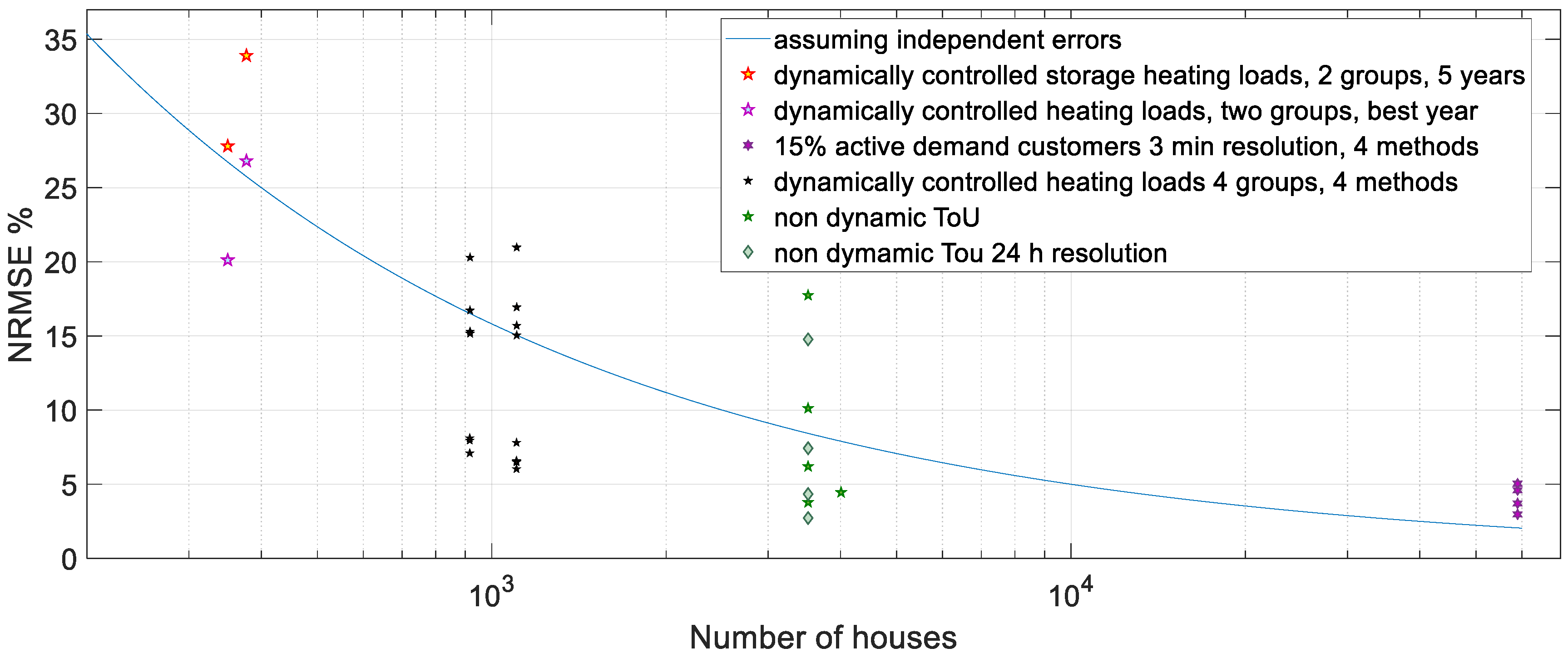Figure 3 demonstrates some of the dependencies. It summarizes some results from our past publications between the years 2012 and 2020. All these publications can be found via [11,16]. All the most accurate methods in Figure 3 are hybrids that combine several short-term forecasting methods and include both machine learning and physically based models. In the case with about 59,000 customers, the most accurate method includes also a similar day method. All of the most accurate methods use more than one hybridization approach, including residual hybrid, ensemble and range constraining.

In Figure 3, the four markers on the right end represent different forecasting method applied to the exact same case. At about 1000 aggregated customers, there are combinations of four rather similar groups of about 1000 customers and two different methods in all eight combinations. The blue line in the figure shows how the forecasting accuracy measured in std. depends on the number of customers assuming completely independent forecasting errors. The expected behavior of uncorrelated forecasts is like that. The cases are not fully comparable and the amount of them is too small for making any reliable conclusions. Forecasting when active loads are not present is usually more accurate than when dynamic load control is applied. Load control also makes the load behavior strongly correlated, which also tends to increase the correlation of forecasting errors and thus reduce the NRMSE improvement stemming from increasing the number of aggregated customers. In the cases with 59,000 customers at the right side of Figure 3, the forecasting time resolution was 3 min and in the other cases it was 1 h. In the lowest NRMSE case at about 3500 customers, it was 24 h. Using more accurate time resolution causes higher values of criteria. At about 3500 customers, the range of the values shows the impact of the improvement of the methods when the case remains the same. There, the outdated national load profiles had the highest NRMSE. In the four groups that have about 1000 customers, the controllable loads dominate. With two of these four groups, the forecasting performance is very good as compared to the blue line. The two leftmost groups, each having 350 to 380 customers, suffered from communication failures in the first third of the 5-year-long verification period. Selecting only the best year of the verification would have given NRMSE = 20.1% for group 1 and NRMSE = 26.8% for group 2 of that case.

One observation is that the results are not always very well comparable between different groups in the same case, nor between different years for the same group. Thus, meaningful comparison of methods across different individual forecasting cases does not seem feasible. The comparability was even worse when using MAPE instead of NRMSE. In addition, the results support the hypothesis that with the best forecasting methods in the studied cases the assumption of mutually independent forecasting errors may be justified if the number of houses is not very large. The amount of cases is too small for making firm conclusions. When the forecasting cases represent the same time and country the cross correlation can be calculated from the forecasts. We leave that now to further studies. The purpose here is only to show that (1) this kind of analysis may be useful when made with many more cases and (2) the comparison of forecasting methods between different cases is complex and gives only very rough results. Further research with many more cases is needed in order to get reliable quantitative results.

Figure 4 shows how the MAPE and NRMSE depended on each other in 38 short-term forecasts that we have produced in six different forecasting cases. All the forecasts have the same forecasting horizon. The differences in their behavior are rather small. This is the expected result for the errors of accurate forecasts. We expect that the results may be much more different if either low accuracy forecasts or more exceptional situations are included in the comparison. Further studies are needed regarding that.

All those six forecasts that have NRMSE between 15% and 17% are from the same group in the same case but use different forecasting methods. The group behavior in the verification was rather different from the identification. The low MAPE in one of the forecasts may indicate that MAPE there failed to adequately detect the rather large peak load errors caused by the behavior change. That may happen, because the statistical behavior of the errors was not any more normally distributed, as is the case with accurate forecasts.

3.5. Load Peak Sensitive Validation

The most valuable forecasts for peak load can be obtained by modeling the actual costs of forecasting errors in the electricity market, in the distribution grid or in both depending on the purpose of forecasting. For most comparisons, this is not practical, because of the complexity and stochastic nature of the costs as shown before. As the cost of the errors is the fundamental reason for the need for accurate forecasts, it is nevertheless important to have at least a general idea on how the costs form and use criteria that reflect the load peak sensitivity of the costs.

Conventional validation statistics cannot solely guarantee the performance of a model in load peak situations. For instance, the recent study on weather forecast-based short-term fault prediction using a neural network (NN) model [27] showed some inherent limitations of the standard MAPE and mean absolute error (MAE) metrics. MAPE does not work due to existence of zero values, i.e., the absence of network faults. MAE does not properly reflect the model performance thoroughly, e.g., in rare peak events. The high fault rate periods are important to predict in order to temporarily increase preparedness to manage them. On the other hand, the results indicate that the index of agreement (IA) [28] may provide a more robust metric for measuring the model performance, including peak events and for model evaluation and comparison in general:

$$IA=1-\left(\frac{SSE}{{{\displaystyle \sum }}_{i=1}^n{\left(\left|{\widehat{y}}_i-\overline{y}\right|+\left|y_i-\overline{y}\right|\right)}^2}\right)$$

(3)

where $SSE={{\displaystyle \sum }}_{i=1}^n{\left(y_i-{\widehat{y}}_i\right)}^2$, $y_i$ is the true number of faults, ${\widehat{y}}_i$ is the predictied number of faults, $\overline{y}=\frac{1}{n}{{\displaystyle \sum }}_{i=1}^n{y}_i$, $i=\overline{1,n}$, $n$ is the sample size, and IA $\in \left[0,1\right]$, higher values of IA indicate better models.

The study [27] also showed that the resampling/boosting of rare faults peaks in the training data can be used to enhance the ability of an NN model to forecast fault events. Figure 5 demonstrates the results of forecasting all types of faults and faults caused by wind, originally presented in [27].

NN models without resampling do not predict peaks but have better MAE as they are more accurate for samples of fewer faults, which are prevalent in the data. On the contrary, NN models with resampling are less accurate for samples of fewer faults, which makes MAE higher. However, the models with resampling are able to predict large peaks, which is more valuable from the problem perspective. For the prediction of all the considered types of faults and wind faults, higher IA values correspond to models with oversampling, which are better at predicting peaks. Based on the given liner regression, we see that there is still a tendency to underestimate peaks. Anyway, the index of agreement may be useful as an additional criterion also in short term load forecasting that has similarly challenges in assessing the performance of forecasting the load peaks.

One option to the aforementioned standard evaluation metrics are categorical statistics i.e., to evaluate model’s performance in critical load peak situations by discriminating electric load to a category/class (e.g., low and high) and then apply some conventional index for each class separately or only to the peak loads. Discrimination can also be based on variables that affect the load such as the outdoor temperature and electricity market price. Evaluation of the accuracy of the daily peak load forecast is sometimes used as a peak load sensitive criterion.

Accurate peak load forecasting is so important that short term peak loads are often separately forecast, as in [29,30], for example. Peak load forecasting may be less sensitive to the choice of criterion than the forecasting of the full profile, but absolute maximum error (AME) was used in [30] to complement MAPE when comparing forecasting methods. This seems justified although there both criteria rated the compared four methods clearly in the same order.

Based on the discrimination and the contingency table, a set of different standard metrics can be derived including:

• The fraction of correct prediction (true positive rate, TPR)
• the false positive rate, FPR
• the Success Index (SI): SI = TPR − FPR

where TPR is the true positive rate representing the sensitivity of the model (the fraction of correct predictions) and FPR is the false positive rate, representing the specificity of the model. SI is limited to the range of −1, 1 and for a perfect model SI = 1 [31,32,33]. With this approach, it is also necessary to have a category for too high predictions, because otherwise too high peak predictions would not be penalized.

Such categorical statistics including probability of detection (POD), critical success index (CSI) and false alarm ration (FAR) are used, e.g., in wind power ramp forecasting as measures of accuracy for forecasts of sudden and large power changes [34,35]. The detection and forecasting of those events is crucial with regard to power production and load balance. However, the ability of forecasting methods to predict those events remains relatively low for short term operation.

• Probability of detection (POD): POD = TP/TP + FN
• Critical success index (CSI): CSI = TP/(TP + FN + FP)
• False alarms ratio (FAR): FAR = FP/(FP + TP).

A possible way to classify the load to suitable categories could be based on the gradient of the load duration curve. Also, proportions of the observed peak load or time could be considered; for example, those times could be used when the load is over 80% of the peak load or 20% of the highest loads measured.

4. Criteria for other Relevant Aspects than Forecasting Performance

4.1. Estimation of Confidence Intervals for Short Term Load Forecasting

Forecasting peak loads too low increases risks and costs as already discussed. Traditionally, these risks are managed by increasing operational margins depending on the situation and based on experience. The operational margin calculation can be the standard deviation (std.) of the short-term load forecast error tuned by a situation dependent coefficient. Forecast error quantiles are also used instead of the std. as the basis of the estimation of the operational margins, because in rarely occurring exceptional situations, such as extreme peak loads, the error distribution may not be normal. For example, Petiau [36] presented a method to estimate the confidence intervals (CI). It is based on the calculation of quantiles of past forecasting errors. CIs quantify the uncertainty of the forecast.

The estimation of the standard errors can be performed, e.g., using the method of bootstrapping. The bootstrapping is a nonparametric approach based on the re-sampling of the data to produce the distribution of re-sampled validation indices [37].

Probabilistic load forecasts provide even more information for risk assessment. Hong and Fan [38] reviewed the methods to produce and evaluate probabilistic forecasts.

Estimation of confidence intervals and the assessment of forecasting performance in exceptional situations are closely related. They both need to focus on exceptional situations where the general assumptions well justified for the errors of accurate forecasts may not be valid.

4.2. Computational Time

In the model identification, many new forecasting methods need much computational resources. This can be problematic, when online learning is applied. For some methods, this is a relevant problem also in off–line model identification, especially because the models need to be updated due to changes in the grid, market aggregation, customer behavior, new priorities, etc. For example, support vector regression (SVR) has so poor computational scalability that it limits the possibilities to exploit it in 1 or 3 min time resolution short-term forecasting needed in electricity grid operation [11]. Based on a brief discussion and comparison of computation times of their models in short term forecasting, Lusis et al. [4] concluded that model run time in model training may be an important factor when choosing between models.

Overly detailed models that have many parameters have poor forecasting performance as the classical textbooks of system identification, such as [39], have shown. In a different application area, a rather recent comparison of several popular statistical and machine learning methods [40] found out that the methods with the best forecasting performance also had the lowest run time computational complexity. Thus, we conclude that if a forecasting method needs excessive computational resources during operation, it is a sign that it also may have both poor performance and unnecessary computations. That is not always the case, however. Some forecasting methods, such as Gaussian Process Regression models, are more computationally intensive during operation, with no connection to overfitting and produce confidence intervals without the need for bootstrapping, which is a big advantage in the considered short-term load forecasting cases.

Different methods also require very different amounts of working time from different types of experts. Physically based forecasting models require good knowledge of the domain and classical model identification. Many forecasting methods, especially many ML methods, require much expertise and time in the tuning of method parameters and model structure to the specific case. Also, the requirements for preprocessing the data vary.

In order to be able to compare the costs and benefits of the forecasting methods, the computational complexity and the need for expertise and working time need to be assessed in terms of monetary costs. The computational complexity has several dimensions such as the need for computational operations and different types of memory. How easily and efficiently the method suits for parallel processing also affects the cost.

5. Discussion

Electricity market costs caused by the forecast errors are quite stochastic due to the impact of very few very high price peaks. Thus, using the observed market costs as identification and tuning criterion is not feasible as the results of the related case study demonstrate.

The results suggest that improving the short-term forecasting accuracy of the aggregated active demand loads further from our best recent methods [11] now may not give adequately significant savings in the expected value of the imbalance costs to justify much method development investments. It seems more important to mitigate the risks caused by high imbalance price peaks. A possible reason is that the one-price consumption imbalance fees of the case study may not reflect adequately the costs of imbalance to the power system. A more important reason is that the forecasting errors of the aggregated distributed flexible load are rather independent and small as compared to the forecasting errors of the overall balance of the balance responsible party responsible for the flexible load.

In the electricity markets, such forecasting errors that are much smaller than the balancing errors of the actor or its balance responsible party have very small impact on the total balancing error. Thus, it is much more important to focus on large errors of the component forecasts. With them, the balancing error costs depend typically linearly on the size of the balancing error. The balancing error costs depend on the related rules and prices of the particular electricity market but in general they tend to reflect only marginal linearized costs in the powers system, when the balancing errors are assumed not to affect the prices. The actual costs for the system operator grow much faster than linearly and that may be the actual case for the competitive market actors if the impacts on balancing power price and risk–hedging costs are not ignored.

In power distribution networks, the costs of forecasting errors concentrate very much on the load peaks of the network. Network losses depend on the square of the current. The aging of the components is rapidly sped–up by temperature increase caused by the losses. Thus, during low load, the impact of load forecast errors is insignificant. During high load peaks, the load forecasting error requires additional operational margin that is expensive. Thus, it is crucial to focus on the forecasting errors during network peak loads that may be at times that are different from times of the peaks of the component load forecast.

Here our focus is in model verification and validation criteria. In model identification or learning there are more limitations regarding the type of the performance criteria. Some model identification methods or tools may accept only certain criteria types. Some others do not have such strict limitations, but the form and properties of criteria always affect convergence and computational efficiency together with the identification model and method.

It was shown that the actual cost of short-term load forecasting errors is a highly non-linear and asymmetric function of the forecasting error. For example, the penalties for underestimating the load should be higher than for overestimating it. The cost of the errors is also highly load-dependent. Arguably, the right thing to do would be to construct a loss function that is specific to the forecasting problem at hand, and have the machine learning optimize that domain-specific loss function directly. Here we only propose, using domain-specific criteria to complement or refine a common loss function such as RMSE rather than replacing it completely. We do not yet experiment with such domain specific load functions, but only aim to explain what they should include and why they are needed. Many standard forecasting packages may not yet support the possibilities to use domain specific loss functions and adding them there could make them better available to more practitioners. The properties of the loss function affect the properties and number of the solution and the convergence of the method identification. These are difficult to assess if there is no analytic form of the loss function available. We show in Section 3.1 why the prices of the electricity markets and ancillary service markets are not directly applicable in a domain specific loss function, because rarely occurring and very unpredictable price peaks dominate the value of the loss function. Similarly, most of the grid costs tend to concentrate to a very few short overload periods. Thus, domain specific loss functions for the short-term load forecasting model identification may create substantial potential risks. The domain specific loss functions need to be designed and considered carefully. We initially assume that directly using domain specific load functions in identification should be used in parallel with other approaches rather than instead of them. Then the good and weak sides of the approaches can be better detected, and the strengths of the different approaches combined. Experimenting with the use of problem-specific loss functions also in the learning phase is a topic worth considering for future research.

6. Conclusions

The main findings were evident but also way too often ignored. (1) It is important to consider the actual costs and other consequences of the prediction errors when selecting criteria for short term load forecasting. (2) The behavior of the actual costs can be very nonlinear. Even quadratic cost criteria may underestimate the growth of the costs with the size of the error and the load peak. (3) Often, the costs stem mainly from peaks in the loads and in the market prices. For such cases, criteria that normalize each error to the simultaneous measurement, such as MAPE, can be very misleading. (4) The results do not support using any of the commonly used criteria to compare methods across different short-term forecasting cases. (5) The costs in real application cases may be so stochastic that their direct use in validation may not be appropriate. (6) Model development effort, expertise need, and computational complexity are also often relevant when selecting short term forecasting methods.

The research results by the authors suggest that integrating different short-term forecasting methods together into hybrids can combine their mutual strengths, thus improving performance and robustness without excessive development effort. The main challenge of such model integration is that it requires expertise with many different modelling methods.

Our aim was to show that the selection, development and analysis of the performance criteria deserves attention. Blindly using so-called standard criteria may mislead the development, tuning and selection of the short-term forecasting methods in real applications.

References

1. Bessa, R.J.; Miranda, V.; Botterud, A.; Wang, J. ‘Good’ or ‘bad’ wind power forecasts: A relative concept. Wind Energy 2011, 14, 625–636. [Google Scholar] [CrossRef]
2. Frances, P.H. A note on the Mean Absolute Scaled Error. Int. J. Forecast. 2016, 32, 20–22. Available online: https://doi.org/10.1016/J.IJFORECAST.2015.03.008 (accessed on 5 February 2020). [CrossRef] [Green Version]
3. Schreck, S.; de la Comble, I.P.; Thiem, S.; Niessen, S. A methodological framework to support load forecast error assessment in Local energy markets. IEEE Trans. Smart Grid 2020. [Google Scholar] [CrossRef]
4. Lusis, P.; Khalipour, K.R.; Andrew, L.; Liebman, A. Short–term residential load forecasting: Impact of calendar effects and forecast granularity. Appl. Energy 2017, 205, 654–669. [Google Scholar] [CrossRef]
5. Hodge, B.; Lew, D.; Milligan, M. Short-term load forecast error distributions and implications for renewable integration studies. In Proceedings of the 2013 IEEE Green Technologies Conference (Green Tech), Denver, CO, USA, 4–5 April2013; pp. 435–442. Available online: https://doi.org/10.1109/GreenTech.2013.73 (accessed on 20 February 2020).
6. Abdulla, K.; Steer, K.; Wirth, A.; Halgamuge, S. Improving the On–line Control of Energy Storage via Forecast Error Metric Customization. J. Energy Storage 2016, 10, 51–59. [Google Scholar]
7. Haben, S.; Ward, J.; Greetham, D.V.; Singleton, C.; Grindrod, P. A new error measure for forecasts of household-level, high resolution electrical energy consumption. Int. J. Forecast 2014, 30, 246–256. [Google Scholar] [CrossRef] [Green Version]
8. Hyndman, R.J.; Koehler, A.B. Another look for measures of forecast accuracy. Int. J. Forecast 2006, 22, 679–688. [Google Scholar] [CrossRef] [Green Version]
9. Jakob, M.; Neves, C.; Vukanovic’Greetham, D. Short Term Load Forecasting. In Forecasting and Assessing Risks of Individual Electricity Peaks; Mathematics of Planet Earth; Springer: Cham, Switzerland, 2020; pp. 33–34. [Google Scholar]
10. Lococ, J.; Beeks, C.; Seidl, T.; Skopal, T. Paramterized Eart Movers Distance for Efficient Metric Space Indexing. In Proceedings of the SISAP ’11, Lipari, Italy, 30 June–1 July 2011; p. 2. [Google Scholar]
11. Koponen, P.; Niska, H.; Mutanen, A. Mitigating the Weaknesses of Machine Learning in Short–Term Forecasting of Aggregated Power System Active Loads. In Proceedings of the IEEE INDIN19, Helsinki–Espoo, Finland, 22–25 July 2019; p. 8. [Google Scholar]
12. Ding, D.; Zhang, M.; Pan, X.; Yang, M.; He, X. Modelling Extreme Events in Time Series Prediction, KDD’19. In Proceedings of the 25th ACM SIGKDD International Conference on Knowledge Discovery & Data Mining, Anchorage, AK, USA, 4–8 August 2019; pp. 1114–1122. Available online: https://doi.org/10.1145/3292500.3330896 (accessed on 11 February 2020).
13. Two-Price and One-Price System, Fingrid. Available online: https://www.fingrid.fi/en/services/balance-service/description-of-balance-model/two-price-and-one-price-system/ (accessed on 11 February 2020).
14. Nord Pool. Elspot Day-a-Head Electricity Prices. Available online: https://www.nordpoolgroup.com/Market-data1/Dayahead/Area-Prices/ALL1/Hourly/?view=table (accessed on 11 February 2020).
15. Fees, Fingrid. Available online: https://www.fingrid.fi/en/services/balance-service/fees/ (accessed on 15 April 2020).
16. Koponen, P.; Salmi, T.; Evens, C.; Takala, S.; Hyttinen, A.; Brester, C.; Niska, H. Aggregated forecasting of the load control responses using a hybrid model that combines a physically based model with machine learning. In Proceedings of the CIRED 2020 Workshop, Berlin, Germany, 22–23 September 2020; p. 4. [Google Scholar]
17. SmartNet. Available online: http://smartnet-project.eu/ (accessed on 15 April 2020).
18. Strbac, G.; Djapic, P.; Pudjianto, D.; Konstantelos, I.; Moreira, R. Strategies for Reducing Losses in Distribution Networks; Imperial College: London, UK, 2018; p. 87. [Google Scholar]
19. Husnayain, F.; Latif, M.; Garniwa, I. Tranformer Oil Lifetime Prediction Using the Arrhenius Law Based on Physical and Electrical Characteristics. In Proceedings of the IEEE 2015 International Conference on Quality in Research, Lombok, Indonesia, 10–13 August 2015; pp. 115–120. [Google Scholar]
20. Bowler, N.; Liu, S. Aging mechanisms and monitoring of cable polymers. Int. J. Progn. Health Manag. 2015, 6, 12. [Google Scholar]
21. Koskela, J.; Rautiainen, A.; Järventausta, P. Utilization possibilities of electrical energy storages in households’ energy management in Finland. Int. Rev. Electr. Eng. 2016, 11, 607–617. [Google Scholar] [CrossRef]
22. Koskela, J.; Lummi, K.; Mutanen, A.; Rautiainen, A.; Järventausta, P. Utilization of electrical energy storage with power-based distribution tariffs in households. IEEE Trans. Power Syst. 2019, 34, 1693–1702. [Google Scholar] [CrossRef]
23. Lummi, K.; Rautiainen, A.; Järventausta, P.; Heine, P.; Lehtinen, J.; Hyvärinen, M.; Salo, J. Alternative power-based pricing schemes for distribution network tariff of small customers. In Proceedings of the IEEE Innovative Smart Grid Technologies-Asia (ISGT Asia), Singapore, 22–25 May 2018; p. 6. [Google Scholar]
24. Mutanen, A. Improving Electricity Distribution System State Estimation with AMR-Based Load Profiles; Tampere University of Technology: Tampere, Finland, 2018; p. 91. [Google Scholar]
25. Humeasu, S.; Wijaya, T.K.; Vasirani, M.; Aberer, K. Electricity load forecasting for residential customers: Exploiting aggregation and correlation between households. In Proceedings of the 2013 Sustainable internet and ICT for sustainability, SustainIT, Palermo, Italy, 30–31 October 2013; Available online: http://dx.doi.org/10.1109/SustainIT.2013.6685208 (accessed on 18 April 2020).
26. Koponen, P.; Mutanen, A.; Niska, H. Assessment of some methods for short–term load forecasting. In Proceedings of the IEEE PES ISGT Europe 2014, Istanbul, Turkey, 12–15 October 2014; p. 6. [Google Scholar]
27. Brester, C.; Niska, H.; Ciszek, R.; Kolehmainen, M. Weather-based fault prediction in electricity networks with artificial neural networks. In Proceedings of the IEEE World Congress on Computational Intelligence (WCCI) 2020, Glasgow, UK, 19–24 July 2020. [Google Scholar]
28. Willmott, C.J.; Ackleson, S.G.; Davis, R.E.; Feddema, J.J.; Klink, K.M.; Legates, D.R.; O’Donnell, J.; Rowe, C.M. Statistics for the evaluation and comparison of models. J. Geophys. Res. 1985, 900, 8995–9005. [Google Scholar] [CrossRef] [Green Version]
29. Sarduy, J.R.G.; Di Santo, K.G.; Saidel, M.A. Linear and non-linear methods for prediction of peak load at University of São Paulo. Measurement 2016, 78, 187–201. Available online: https://doi.org/10.1016/J.MEASUREMENT.2015.09.053 (accessed on 18 April 2020). [CrossRef]
30. Grant, J.; Eltoukhy, M.; Asfour, S. Short-Term Electrical Peak Demand Forecasting in a Large Government Building Using Artificial Neural Networks. Energies 2014, 7, 1935–1953. [Google Scholar] [CrossRef] [Green Version]
31. Youden, W.J. Index for rating diagnostic tests. Cancer 1950, 50, 32–35. [Google Scholar] [CrossRef]
32. Van Aalst, R.M.; De Leeuw, F.A. European Topic Centre on Air Quality (RIVM, NILU, NOA, DNMI). In National Ozone Forecasting Systems and International Data Exchange in Northwest Europe; Report of the Technical Working Group on Data Exchange and Forecasting for Ozone Episodes in Northwest Europe (TWG-DFO)); European Environment Agency: København, Danmark, 1997. [Google Scholar]
33. Gajowniczek, K.; Ząbkowski, T. Short Term Electricity Forecasting Using Individual Smart Meter Data. Procedia Comput. Sci. 2014, 35, 589–597. [Google Scholar] [CrossRef] [Green Version]
34. Ferreira, C.; Gama, J.; Matias, L.; Botterud, A.; Wang, J. A Survey on Wind Power Ramp Forecasting; Technical Report No. ANL/DIS-10-13; Argonne National Laboratory: Lemont, IL, USA, 2010. [Google Scholar]
35. Zhang, J.; Florita, A.; Hodge, B.-M.; Freedman, J. Ramp forecasting performance from improved short-term wind power forecasting. In Proceedings of the ASME 2014 International Design Engineering Technical Conferences & Computers and Information in Engineering Conference IDETC/CIE 2014, Buffalo, NY, USA, 17–20 August 2014; p. 12. [Google Scholar]
36. Petiau, R.B. Confidence interval estimation for short-term load forecasting. In Proceedings of the 2009 IEEE Bucharest PowerTech, Bucharest, Romania, 28 June–2 July 2009; pp. 1–6. [Google Scholar]
37. Efron, B.; Tibshirani, R.J. An Introduction to the Bootstrap; Chapman and Hall: New York, NY, USA, 1993. [Google Scholar]
38. Hong, T.; Fan, S. Probabilistic electric load forecasting: A tutorial review. Int. J. Forecast. 2016, 32, 914–938. Available online: https://doi.org/10.1016/J.IJFORECAST.2015.11.011 (accessed on 18 April 2020). [CrossRef]
39. Ljung, L. System Identification, Theory for the User, 2nd ed.; Prentice Hall: Upper Saddle River, NJ, USA, 1999; p. 640. [Google Scholar]
40. Madridakis, S.; Spillotis, E.; Assimakopoulos, V. Statistical and Machine Learning forecasting methods: Concerns and ways forward. PLoS ONE 2018, 13, 26. [Google Scholar]
Figure 1. (a) Impact of an additional error std. component to the total error std. when assuming normally distributed independent error sequences, (b) the behavior of the mean of simulated balancing error costs, (c) the range of balancing error cost variation in the simulations.
Energies 13 02054 g001
Figure 2. Percentage yearly savings of customers when using energy storage to decrease monthly maximum peak powers and the costs of market priced energy, shown as a function of different forecast error criteria. Color of points shows the used error level (0–200%).
Energies 13 02054 g002
Figure 3. Load forecasting accuracy as a function of the number of aggregated customers as collected from our own published results. The results support the assumption of independent errors except for the largest group size and the other differences reduce the comparability among the cases much more.
Energies 13 02054 g003
Figure 4. Comparison of normalized root mean squared error (NRMSE) and mean absolute percentage error (MAPE) in 38 forecasts in 6 different short term load forecasting cases comprising together 12 different forecasting methods.
Energies 13 02054 g004
Figure 5. Weather-based fault prediction in the electricity network: comparison of NN models in two experiments with and without resampling. (a) All faults, (b) Faults caused by wind.
Energies 13 02054 g005