1. Introduction
All over the world, power transmission grids are suffering issues such as power-line congestions or voltage instability due to rising consumption and the inclusion of new distributed and unmanageable generators, mainly PV generators and WPP [
1]. These situations lead to a crossroads in regard to the aim of power systems planners to ensure the availability of a reliable electrical supply.
Voltage instability occurs when power systems are unable to meet the demand for reactive power. The main obstacle to power flow is power losses caused by line impedances, which lead to voltage drops [
2]. Therefore, any variation in line impedances, or any reduction of available paths from generators to loads, may affect voltage profile and harm voltage stability. Furthermore, the active power that can be transmitted through an impedance from a constant voltage source is physically limited [
2]. Thus, any load shift or rise may also modify both the voltage profile and voltage stability margin.
These problems might be solved by setting new power plants and transmission lines or repowering the existing ones. However, these approaches involve lengthy construction times, large investments and various environmental, legal and social difficulties [
3], especially in small territories, such as islands. Alternatively, a new solution to this operational problems has arisen from power electronics following the development of the first FACTS devices in the 1980s [
4].
FACTS are Alternating Current transmission systems based on power electronics and other static controllers intended to control power networks in a flexible manner [
5]. FACTS controllers are static equipment, mainly power electronic-based devices, that provide control of one or more AC transmission systems parameters.
In recent decades, great efforts have been made to augment both loading capability and voltage stability of existing power systems by using FACTS devices.
Size and location are key to an optimal use of FACTS devices. Nonetheless, several studies have demonstrated that finding the best solution to this problem is not an easy task. Some authors proved that, in certain cases, the weakest bus is not the best location for compensation in terms of voltage stability enhancement [
6]. Furthermore, others have found that the need for reactive power is determined by the required capacity under contingency state [
7].
Researchers have employed and combined different techniques in order to study the effects of the inclusion of this technology in power systems operation. Most of them are based on one of the different PF methods, namely: PF ([
8,
9]), OPF [
10], CPF ([
11,
12]) or VSCOPF [
13].
The main focus of these studies is to determine the best location and size of the FACTS device (or devices). The objective function is often defined in terms of maximising voltage stability and minimising voltage deviation, power losses or costs. Voltage stability can be either calculated using PV studies [
8] or CPF [
11], or estimated, using eigenvalues-based methods [
6], index-based methods ([
9,
14]), modal analysis techniques [
15] or trajectory sensitivity analysis [
16]. Alternatively, some authors establish an economical scope on their studies by optimizing generation costs [
17], fuel costs [
18], operation costs [
19] or the NPC [
20].
In recent years there has been growing interest in the employment of AI to this kind of problems. Actually, AI techniques such as PSO, GA, GSA or DE have inspired researchers to develop several algorithms ([
21,
22,
23]). Alternatively, the Pareto approach, combined with FDMs, is also employed to determine the optimal FACTS devices allocation [
24].
The main limitation of these procedures is that they are usually based on one snapshot of the power system, since they only take into account a single network configuration, load share, generation dispatch, etc. Another classical approach to power system planning problems is focused on peak and valley demand points, which in the end, entails the same limitations.
In
Table 1 a brief survey on FACTS devices allocation procedures focusing on system configuration is shown. As it can be seen, only one of them takes into account demand variations (as well as generation), while two of them take into account contingency states.
As mentioned in [
17], the presence of some types of renewable generators in the power system entails the risks of their intermittence. This can have an important effect on the results of the placement procedure. In fact, the authors have noted an inconsistency with classical methodologies, since they have demonstrated that peak demand is not always the best system configuration for running a FACTS allocation solver, since it may not ensure the optimal solution.
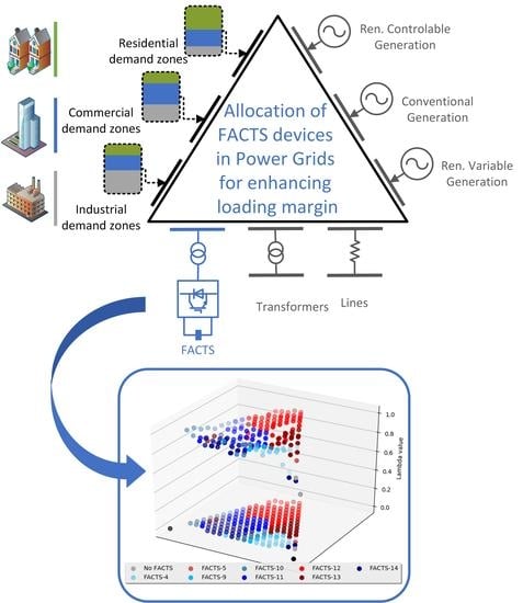
The objective of the present paper is to demonstrate that the results obtained from FACTS devices allocation studies may vary, depending on load share. Several demand scenarios were created so as to study their influence on FACTS devices allocation. Additionally, a new approach to FACTS devices allocation is given. We have modified the multiobjective optimisation proposed in [
25] in order to assess this problem taking load share into account. By doing so, loading margin was maximised and voltage deviation and reactive power losses were minimised using a modified IEEE 14-bus test system [
26].
This document is organised as follows. The mathematical formulation of the problem is described in
Section 2 and the methodology developed in this project and the simulator used to test it are depicted in
Section 3. Finally, results are presented in
Section 4 and discussed in
Section 5, while conclusions are drawn in
Section 6.
2. Problem Formulation
2.1. Load Influence on Line Compensation
In its simplest form, the FACTS devices allocation problem can be reduced to a single phase line compensation problem, since a loss-less power line with distributed parameters is ruled by Equations (
1) and (
2) [
2].
where
and
represent voltage and current at a distance
x from the sending end of the line,
is the phase constant of the electrical wave,
and
represent voltage and current at the receiving end and
is the characteristic impedance of the line.
On the one hand, if we substitute
x by the length of the line (
L), we can calculate voltage and current at the sending end. This means that
and
. On the other hand, if a voltage source is connected to the sending end of the line and the receiving end is open-circuited, the current at the receiving end is
, and the voltage at the receiving end is much higher than at the sending end,
. Nevertheless, if we close the line with its
, its voltage and current magnitudes remain constant along its length (flat line) [
2], since its reactance is compensated.
When the line is connected to sources of identical voltage at both ends, and , since both currents are entering the line. Therefore, following the principle of symmetry, the current must become zero at half the length of the line (). In such a situation, we can treat each half of the line as an open-circuited line. Consequently, a loss-less power line connected to identical voltage sources in both ends may be compensated by half of its at its midpoint.
Given this, we tried to figure out if the Theoretical Point of Compensation (TPoC) may move along the line as long as its loading conditions changes. According to Equation (
2), if
we can calculate
x, which represents the point in which a line fed by both ends may be compensated.
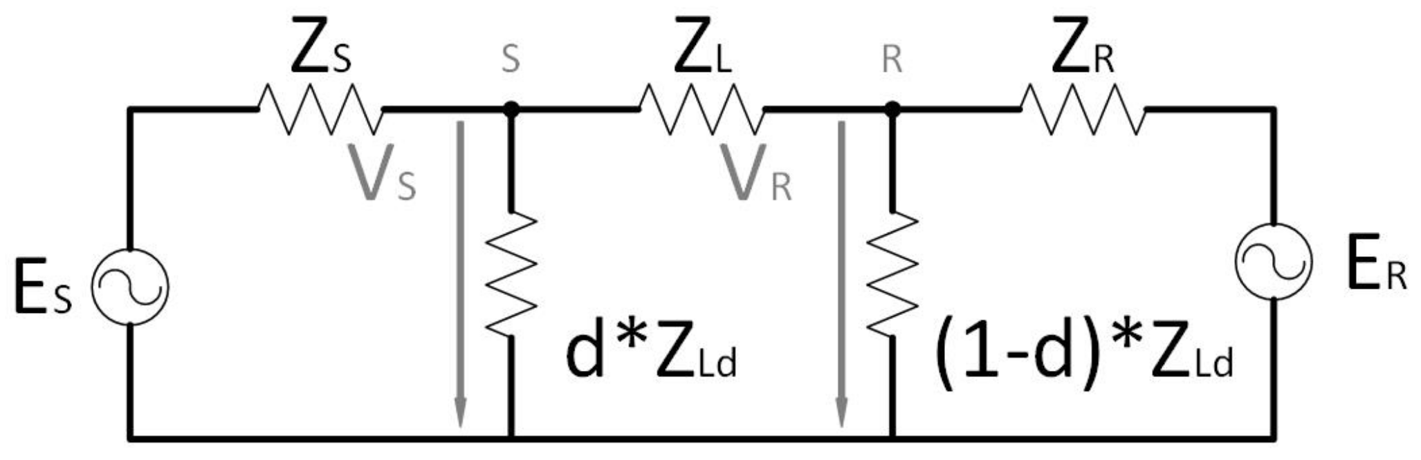
With this in mind, we have created a model that emulates a power line connected to identical voltage sources at both ends via shunt impedances (
and
) (
Figure 1). If
, shunt impedances at both ends of the line are equal. Hence,
and
at
. In contrast, if
d does not equal
, shunt impedances are not equal,
does not equal
and
at
. In other words, depending on the balance of load at both ends of the line, the TPoC may take several positions along the line following a lineal relationship.
Finally, we can generalise the problem to
n lines by generalising Equations (
1) and (
2) and making the aforementioned assumptions (Equations (
3) and (
4)).
where
i and
k are nodes linked by the line whose parameters are denoted with
.
2.2. PV Analysis
As we have seen, the simplest case of power system can be represented as a constant voltage source that feeds a load through an impedance. In such a situation, there is a maximum value of active power that can be transmitted for a fixed power factor (
Figure 2). For any value of active power at the receiving end (
) such as
, we can find two operating points. On the one hand, at the upper point (
A), any decrease in
results in an increase of
. On the other hand, at the lower point (
B), any decrease in
results in a decrease of
. Since voltage controllers are designed to operate in region
A, when operating in region
B the system becomes unstable. Hence, the conditions in which
represent the limit of satisfactory operation. The values of voltage and current corresponding to that point (
C) are referred to as critical values [
2]. When dealing with complex power systems, the situation in which the voltage in one or more nodes inevitably falls is referred to as voltage collapse.
Using PF methods, we can calculate the critical values in which voltage collapse occurs for a given power system. Starting from a given loading level (
), load is iteratively increased (and PF is calculated) until the voltage collapse occurs (
). Thus, loading margin (
) can be defined as:
2.3. Multiobjective Max-Min Optimisation
A multiobjective problem can be solved as a max-min optimisation problem, which implies a worst-case scenario approach [
27]. This approach is particularly appropriate for power system planning studies due to the magnitude of investments as well as the criticality of electrical facilities.
In the context of the problem of this paper, the max-min optimisation problem can be stated as:
where
are the
n objective functions,
are the
m constraints and
V is the decision space.
3. Materials and Methods
In order to assess the importance of load share in FACTS allocation studies, we have developed a methodology that helps us to determine its relationship. The program suitable for testing this methodology can be found in [
28].
3.1. Load Share Scenarios
Firstly, the nodes within the power system are split into three demand zones. By doing so, every load scenario can be identified by its three-dimensional coordinates, referred to as its load share. Using the representation procedure developed in [
29], three-dimensional data can be represented in a two-dimensional space. Demand zones are predefined according to the topology of the grid.
Later on, several load share scenarios are iteratively created by distributing the total system load among the three demand zones. In each iteration, the share of the system load assigned to every demand zone changes by a fixed step, which is defined as a percentage of system load (
). Total system load is iteratively distributed between the different demand zones attending to the restriction in Equation (
8) (
Figure 3).
where
,
and
represent the load in every demand zone and
is the total system load.
The load assigned to every demand zone is distributed among the corresponding nodes respecting its original share.
3.2. FACTS Allocation Procedure
Once a load share scenario is created, the FACTS allocation procedure is initiated. In the first step, a PV analysis is performed to evaluate the voltage stability of the current system configuration without FACTS device. Thereafter, for each of the predefined available locations, the device is set and configured at the corresponding node, and the PV analysis is then reinitialised. This procedure is repeated for each load share scenario, respecting Equation (
8) (
Figure 3).
3.3. Optimisation
From the results of every PV analysis, the Fused Performance Index (
) is calculated (Equation (
15)). The objective of the optimisation procedure is to maximise loading margin (
9) and to minimise voltage deviation (
10) and reactive power loss (
11) using the worst-case criterion. This procedure is based on the one described in [
25]. Nonetheless, changes have been made so as to take load share into account.
The optimal location for FACTS devices is then defined by the optimal (maximum) value of the
, which in turn is determined by the minimum value among the three OFs stated in (
12)–(
14).
In Equation (
13),
is the sum of the deviations of the voltage from its rated value (1 p.u.) at the nodes in which a violation of the voltage limits (0.95–1.05 p.u.) has occurred (Equation (
10)).
The functions used here, except for , refer to a single loading level within the PV analysis. In order to enable comparison among the results for each FACTS device location, the indices must be calculated for the same loading level at every iteration within a load share scenario. Thus, we have determined this to be the maximum loading level handled by the system without FACTS device (base case).
We did not make any assumption about whether maximum or minimum values of , voltage deviation or reactive power loss correspond to the base case or not. This means that these values must be computed and that the base case is treated the same as the available locations. Therefore, it is possible for the optimal choice, at any load share scenario, to be the base case. In other words, it is possible that the best option may be to not install a FACTS device.
Given that the whole space of load share has been sampled, relative frequency (
f) can be used to determine which of the solutions performed better in a greater number of demand scenarios. Therefore, the multiobjective FACTS device allocation problem can be stated so that:
where
l stands for every available location and
L is the set of available locations.
is the Optimal Location for a given load share scenario (
s),
is the Most Frequent Optimal Location and
is the relative frequency of every
l as optimal for different load share scenarios. On the other hand,
g is the equality constraints of load flow equations and
h is the set of system operating constraints so that:
where
n is the number of generators and
m is the number of FACTS devices.
Since the size of the device does not affect the effectiveness of the compensation, we can obviate this parameter within the allocation procedure. Moreover, this is a time-consuming task that can be carried out a posteriori. Consequently, we have considered the size of the FACTS device as a constant in this procedure.
In addition, in order to evaluate the performance of the , we compared its results with those we obtained using itself as an objective function.
3.4. IEEE 14-Bus Test System
In order to test our proposal, we chose a specific type of FACTS device to be placed in a benchmark power system, on which we performed the simulations using PSS-E
® 34 [
30].
The IEEE 14-bus test system (
Figure 4) represents a portion of the American Electric Power System as of February, 1962 [
26]. It is composed of 20 branches, 14 buses, two generators (buses 1 and 2), three synchronous condensers (buses 3, 6 and 8), a capacitive switched shunt (bus 9) and 11 loads. The sum of the loads of this benchmark system is 259 MW and 77.4 MVAr.
The switched shunt in bus 9 has been removed from the system during the calculations so as to make our results comparable with those in [
25] and other papers.
In order to facilitate the understanding of the results, we must provide further information about this research. On the one hand, we must point out that the available locations in which the STATCOM can be set are buses 4, 5, 9, 10, 11, 12, 13 and 14. On the other hand, we must define the three demand zones, which are formed by buses 2 and 3 (demand zone 1), buses 4, 9, 10, 11 and 14 (demand zone 2), and buses 5, 6, 12 and 13 (demand zone 3) (
Figure 4). Transformers between buses 5 and 6 and between buses 4 and 9 serve as boundary of demand zone 1. Demand zones 2 and 3 comprise buses one and two buses away from transformers 4-9 and 5-6 respectively.
3.5. FACTS Device
The STATCOM is a particular type of VSC. It is composed of a capacitor, which acts as a voltage source, and a series of fast electronic switching devices; mainly IGBTs or GTOs (
Figure 5). STATCOMs are intended to dynamically generate or absorb reactive power in a fast and robust way, since no moving parts are involved and low voltages do not affect its operation [
3]. These devices are often connected to a step-up transformer and can be modeled either as a variable voltage source or a synchronous condenser for steady-state studies (
Figure 6).
The STATCOM model has been configurated as follows: = 100 MVA and . Where is the voltage at the bus in which the device is installed at the base case.
4. Results
This section shows the results we have obtained from the simulations. It is worth noting that, in order to represent the results so they can be easily understood, we have used the representation procedure developed in [
29]. The main characteristic of this procedure is that it enables us to represent three-dimensional data, the load share of the three demand zones, into a two-dimensional space, using the interdependence of the variables (Equation (
8)).
The triangle in the figures shows the best location of the STATCOM for each load share scenario. Each corner of the triangle represents the load share scenario in which the total system load is set into only one of the demand zones. Thus, points inside the triangle represent the shift of the load from one demand zone to the others, respecting the restriction stated in (
8). Consequently, the centroid of the triangle coincides with the situation in which the load assigned to every demand zone is the same (
each). The presence of blank spaces in the chart corresponds to the existence of unstable load share scenarios whose Power Flow could not be calculated.
Each point in the chart represents a solution to the allocation procedure based on a load share scenario. At the same time, the colour of each one is referred to the number of the selected bus. It is worth noting that there is no available positions in demand zone 1. Thus, we have grouped the colours that represent the selected nodes in two ranges: we represent nodes from demand zone 2 with blue and nodes from demand zone 3 with red. Furthermore, darker colours represent nodes furthest away from generation (placed in nodes 1, 2 and 3).
The most remarkable conclusion to emerge from the data analysis is that the result of the FACTS allocation procedure often changes, depending on the load share scenario. Nevertheless, contrary to our expectations, we found that the solution drastically changed from one load share scenario to the other (
Figure 7). For this reason, we filtered the results of Equations (
12)–(
14) using a mean filter in order to smooth the variation of the
. At the same time, the values of
have also been filtered.
Regarding the filtered results, we should mention that there are substantial discrepancies between the results of
and
as objective functions. The optimal location for a given load share scenario does not coincide for both indices in most cases nor the frequency of the solutions (
Figure 8).
Using the
as the objective function, the most frequently selected locations were buses 5 and 13, which were chosen in more than
of the load share scenarios. In contrast, using
as the objective function, the most frequent choice was, doubtlessly, bus number 12, which comprises around a third of total solutions. Given these discrepancies, results from both objective functions must be analysed separately. In
Table 2, these results can be compared with those in similar approaches in the literature that, contrarily, do not take load share into account.
It is worth noting that, together with the number of the selected bus, this procedure provides a performance index: or . These two parameters provide different information for decision making. Therefore, the following comparative analysis was carried out on the basis of a graphical marriage between selected bus number and index value attending to the different load share scenarios.
4.1. FPI as Objective Function
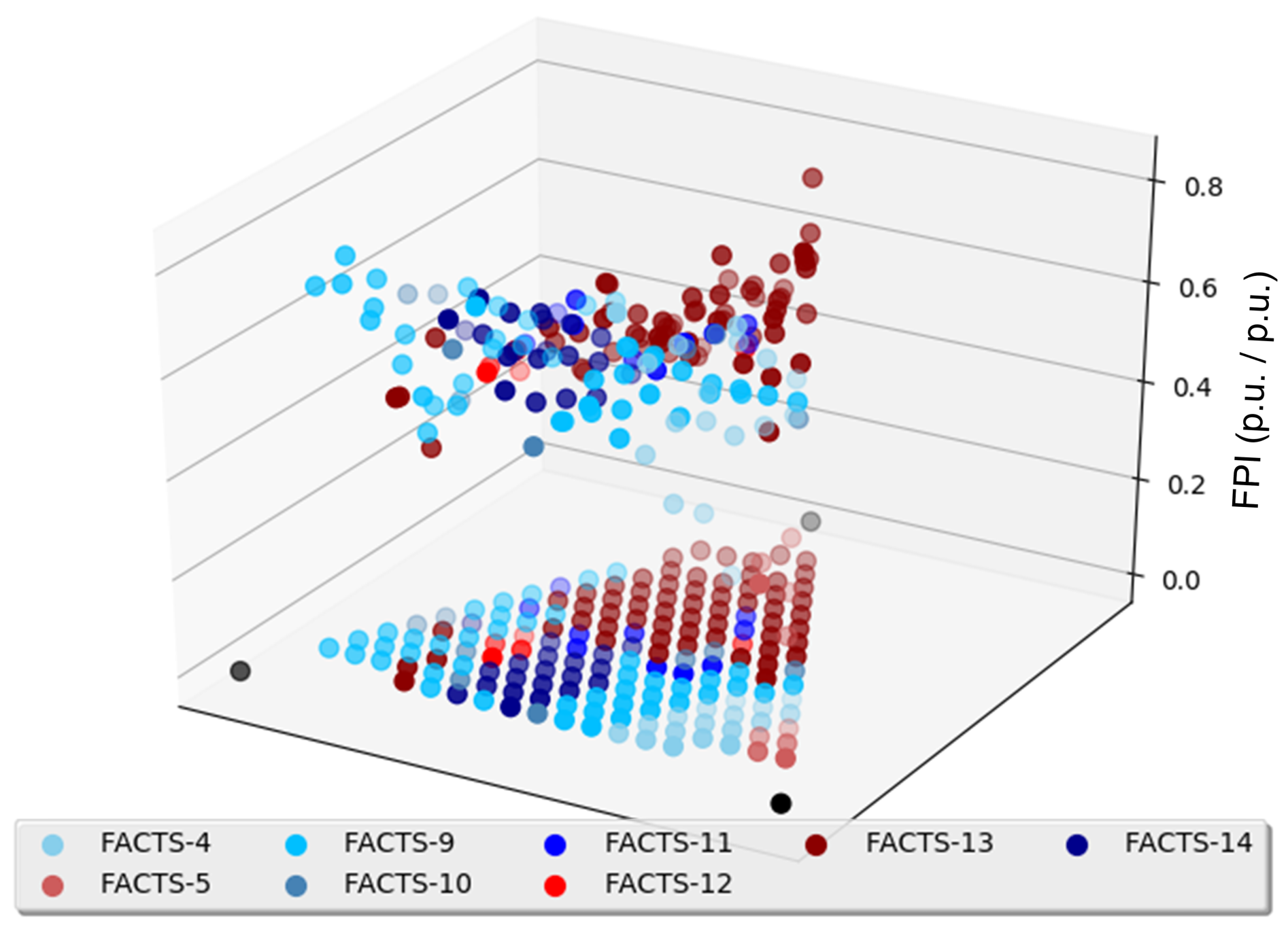
Analysing the
as OF more deeply, we obtained the following results. In regards to which demand zone the nodes belong to, nodes from demand zone 2 (blue colours) were more frequently selected when zones 1 and 2 were overloaded (
Figure 9). More precisely, whenever demand zone 1 becomes more and more loaded, the preferred options become bus number 4 and 5, which are directly linked to the area. This may be due to the fact that there is no available location in demand zone 1. On the other hand, bus number 9 was preferred when demand zone 2 was the most loaded one.
When load shifts to demand zone 3, solutions from the same area (red colours) predominate. In particular, bus number 13 proved to be the most frequent solution in this situation.
Additionally, further analysis has shown that the values of the tended to be dispersed. Focusing on this tendency, we found that their value increased when load shifted to demand zones 2 and 3, while they strongly decreased when load tended to concentrate in demand zone 1.
4.2. Lambda as Objective Function
In a similar manner, when using
as OF, the tests revealed that solutions from demand zone 2 clearly predominated as demand zones 1 and 2 were the most loaded ones (
Figure 10). Nevertheless, in this case, bus number 14 proved to be the most suitable solution when demand zone 2 was overloaded, while bus number 4 proved to be the best choice when load shifted to demand zone 1. Finally, buses from demand zone 3, especially bus number 12, were preferred when load moved to that area.
From a quantitative point of view, the simulations have shown that the values of tended to remain more concentrated than those of the . Nevertheless, they tended to rise when load shifted to demand zone 3. On the contrary, they drastically fell when load approached demand zone 1.
5. Discussion
Although there were some discrepancies between results using different objective functions, we believe our results to be consistent with the expectations.
To begin with, our findings appear to be well supported by previous studies that demonstrate that buses from 9 to 14 are the weakest within the grid ([
25,
31]). Nevertheless, the weakest bus is not always the best choice for compensation [
25]. Moreover, since the effectiveness of voltage regulation is mainly local, it is expected, for FACTS optimal location, to be near the weakest buses. The most frequent locations were bus 13 for
and bus 12 for
.
Secondly, as we have theoretically proven, load has a major impact in FACTS allocation selection. In short, the critical buses in terms of voltage collapse may differ from one demand scenario to the next, since bus load strongly influences bus voltage. Therefore, FACTS optimal location is expected to approach to the most loaded areas.
Remarkably, the results we obtained seem to follow this double correlation. On the one hand, the most selected buses coincide with the weakest ones. On the other hand, the selected bus tended to be within, or in the vicinity of, the most loaded demand zone.
Apart from that, even though their behaviour differs, both indices captured the effect of the absence of available locations in demand zone 1. While tended to remain more stable, the tended to fluctuate, augmenting when load concentrated in demand zones 2 and 3. Nevertheless, when load shifted to demand zone 1, both indices values sank.
In addition, despite there being no good agreement between results using different objective functions at a bus level, it is at a demand zone level. Buses from demand zone 2 proved to be preferred when load shifted to demand zones 1 and 2, while buses from demand zone 3 performed better when their zone was overloaded. Taken together, these results would seem to suggest that both and work well for FACTS devices placement. Despite, they have different meanings. On the one hand, indicates how much load can grow in a safe manner, so it is suitable for mid and long term planning. On the other hand, also takes into account operation variables, such as voltage and reactive power loss. It depends on the scope of the study being performed which one should be used by decision makers.
Finally, since our procedure is based on typical power system parameters (loading margin, voltage and reactive power losses), our findings can be generalised. Given the influence of load share on FACTS devices allocation, our results support the idea that the system demand peak may not be the best choice as a base case for these studies [
17]. Moreover, studying a single system configuration may not be enough to ensure a reliable solution.
6. Conclusions
In this paper we have investigated the influence of the load share in the process of optimally placing FACTS devices. Given this objective, we have modified the method proposed in [
25] and applied this to the IEEE 14-bus test system so as to estimate the optimal location for a FACTS device (STATCOM). Next, we have created several load share scenarios and iteratively repeated the optimisation process.
This study has revealed that care must be taken in order to ensure a reliable result when dealing with power system planning studies. Above all, we have proven that load share strongly affects the result of the FACTS device allocation procedure. Moreover, we have proven that the objective function used may also affect the results at a bus level.
Our work has led us to the general conclusion that load share has a major influence in FACTS devices allocation. In particular, in spite of the objective function used, we found that: (a) the weakest buses were more frequently selected, (b) the preferred buses were inside, or in the vicinity of, the most loaded areas. Nevertheless, we have outlined and discussed the discrepancies and similarities between results of the and as objective functions within the optimisation process.
Depending on the objective function, the optimal solution differs. The provides bus 13 as the most frequent choice, while determines bus 12 as the most preferred one.
From a wider point of view, our study entails a new perspective in power system planning studies. This approach encourages system planners to perform deeper and wider tests when facing these problems. In order to ensure a reliable solution, they must assess the influence of distinct objective functions and, especially, load share in planning studies.
For these reasons, this research could be a useful aid for decision makers and system planners, since it clarifies how load share, as well as some objective functions, affect the results of these studies.
At last, it is worth pointing out that not all load share scenarios are equally likely. Given their influence on the final result, it is important to take their probability of occurrence into account in future studies.
Author Contributions
Conceptualization, S.M.V., I.N. and M.H.-T.; methodology, S.M.V., I.N. and M.H.-T.; software, S.M.V.; validation, S.M.V. and I.N.; formal analysis, I.N. and M.H.-T.; investigation, S.M.V.; resources, I.N. and M.H.-T.; writing—original draft preparation, S.M.V.; writing—review and editing, I.N. and M.H.-T.; visualization, S.M.V.; supervision, I.N.; project administration, I.N. and M.H.-T.; funding acquisition, I.N. and M.H.-T. All authors have read and agreed to the published version of the manuscript.
Funding
This research received no external funding.
Acknowledgments
S. Marrero is the recipient of a grant from the Training Program for Predoctoral Research Staff of University of Las Palmas de Gran Canaria, funded by Cabildo de Gran Canaria. The authors are grateful for this support. Neither this research nor an analysis plan have been preregistered in any independent institutional registry. The authors would also like to thank the anonymous reviewers for their thoughtful comments and efforts towards improving our manuscript.
Conflicts of Interest
The authors declare no conflict of interest.
Abbreviations
The following nomenclatures are used in this manuscript:
| Acronyms |
| FACTS | Flexible Alternating Current Transmission Systems |
| PV | Photovoltaic |
| WPP | Wind Power Plant |
| PF | Power Flow |
| OPF | Optimal Power Flow |
| CPF | Continuation Power Flow |
| VSCOPF | Voltage Stability Constrained Optimal Power Flow |
| NPC | Net Present Cost |
| AI | Artificial Intelligence |
| PSO | Particle Swarm Optimization |
| GA | Genetic Algorithm |
| GSA | Gravitational Search Algorithm |
| DE | Differential Evolution |
| MCS | Monte Carlo Simulation |
| S-AFA | Self-Adaptive Firefly Algorithm |
| -CM | Epsilon-Constrained Method |
| OF | Objective Function |
| OM | Optimization Method |
| FDM | Fuzzy Decision Method |
| L | line Length |
| TPoC | Theoretical Point of Compensation |
| x | distance from the line’s sending end |
| Worst-Case Decision |
| Optimal Solution |
| Most Frequent Optimal Location |
| Optimal Location for a FACTS device |
| g | set of Power Flow equality constraints |
| h | set of power system operating constraints |
| v | vector of dependent variables |
| u | vector of independent variables |
| P | Power (W) |
| V | Voltage (V) |
| I | Current (A) |
| Z | impedance () |
| S | apparent power (MVA) |
| Fused Performance Index (adm.) |
| Voltage Deviation Index (adm.) |
| Loading Margin Index (adm.) |
| Reactive Power Loss Index (adm.) |
| f | Relative Frequency (p.u.) |
| c | Constraint |
| Voltage Deviation (p.u.) |
| Size | FACTS device rating (MVAr) |
| PL | Active Power Loss (MW) |
| Reactive Power Loss (MVAr) |
| EDC | Expected Damage Cost ($) |
| GC | Generation Costs ($) |
| FC | Fuel Costs ($) |
| C | System Costs ($) |
| L-index | distance from voltage collapse index |
| Ev | Eigenvalues |
| Inv | Investment on FACTS instalation ($) |
| STATCOM | Static Compensator |
| VSC | Voltage Source Converter |
| DSSC | Distributed Static Series Compensator |
| TCSC | Thyristor-Controlled Series Capacitor |
| HFC | Hybrid Flow Controller |
| PST | Phase-Shifting Transformers |
| UPFC | Unified Power Flow Controller |
| SVC | Static Var Compensator |
| IPFC | Interline Power Flow Controller |
| IGBT | Insulated Gate Bipolar Transistors |
| GTO | Gate Turn-Off thyristors |
| Greek letters | |
| phase constant of the electrical wave |
| system loading margin |
| Subscripts | |
| initial loading level |
| Bus |
| C | Compensation |
| l | available Locations for FACTS devices placement |
| Load |
| Maximum |
| Minimum |
| R | line Receiving end |
| Reference value for control |
| S | line Sending end |
| s | load share Scenario |
| System |
| demand Zone |
References
- Hingorani, N.G.; Gyugyi, L. Understanding FACTS; Wiley-IEEE Press: Hoboken, NJ, USA, 1999. [Google Scholar]
- Kundur, P. Power System Stability and Control; McGraw-Hill Inc.: New York, NY, USA, 1993. [Google Scholar]
- Acha, E.; Fuerte-Esquivel, C.R.; Ambirz-Perez, H.; Angeles-Camacho, C. FACTS. Modelling and Simulation in Power Networks; John Wiley & Sons: Hoboken, NJ, USA, 2004. [Google Scholar]
- Sreedharan, S.; Joseph, T.; Joseph, S.; Chandran, C.V.; Vishnu, J.; Das, V. Power system loading margin enhancement by optimal STATCOM integration—A case study. Comput. Electr. Eng. 2020, 81, 106521. [Google Scholar] [CrossRef]
- Edris, A.A. Proposed terms and definitions for Flexible AC Transmission System (FACTS). IEEE Trans. Power Deliv. 1997, 12, 1848–1853. [Google Scholar] [CrossRef]
- Padke, A.R.; Fozdar, M.; Naizi, K.R. A new multi-objective fuzzy-GA formulation for optimal placement and sizing of shunt FACTS controller. Electr. Power Energy Syst. 2012, 40, 46–53. [Google Scholar]
- Wibowo, R.S.; Yorino, N.; Eghbal, M.; Zoka, Y.; Sasaki, Y. FACTS devices allocation with control coordination considering congestion relief and voltage stability. IEEE Trans. Power Syst. 2011, 26, 2302–2310. [Google Scholar] [CrossRef]
- Mahdad, B.; Bouktir, T.; Srairi, K. Strategy of location and control of FACTS devices for enhancing power quality. In Proceedings of the MELECON 2006—2006 IEEE Mediterranean Electrotechnical Conference, Malaga, Spain, 16–19 May 2006. [Google Scholar]
- Rani, M.; Gupta, A. Steady state voltage stability enhancement of Power System using FACTS devices. In Proceedings of the 2014 6th IEEE Power India International Conference (PIICON), Delhi, India, 5–7 December 2014. [Google Scholar] [CrossRef]
- Alabduljabbar, A.A.; Milanovic, J.V. Assessment of techno-economic contribution of FACTS devices to power system operation. Electric Power Syst. Res. 2010, 80, 1247–1255. [Google Scholar] [CrossRef]
- Kamarposhti, M.A.; Soltani, H. The study of Maximun Loading Point in investigation of capacitor performance with power selectronic shunt devices. In Proceedings of the 2009 International Conference on Electrical and Electronics Engineering-ELECO 2009, Bursa, Turkey, 5–8 November 2009. [Google Scholar] [CrossRef]
- Telan, A.; Bedekar, P. Systematic approach for optimal placement and sizing of STATCOM to asses the voltage stability. In Proceedings of the International Conference on Circuit, Power and Computing Technologies (ICCPCT), Nagercoil, India, 18–19 March 2016. [Google Scholar] [CrossRef]
- Roselyn, J.P.; Devaraj, D.; Dash, S.S. Multi-objective Genetic Algorithm for voltage stability enhancement using rescheduling and FACTS devices. Ain Shams Eng. J. 2014, 5, 789–801. [Google Scholar] [CrossRef] [Green Version]
- Albatsh, F.M.; Ahmad, S.; Mekhilef, S.; Mokhis, H.; Hassan, M.A. Optimal placement of Unified Power Flow Controllers to improve dynamic stability using power system variable based voltage stability. PLoS ONE 2015, 10, e0123802. [Google Scholar] [CrossRef]
- Rathi, A.; Sadda, A.; Nebhnani, L.; Maheshwar, V.M.; Pareek, V.S. Voltage stability assessment in the presence of optimally placed D-FACTS devices. In Proceedings of the India International Conference on Power Electronics (IICPE), Delhi, India, 6–8 December 2012. [Google Scholar] [CrossRef]
- Bindeshwar Singh, V. Mujherjee, P.T. A survey on impact assessment of DB and FACTS controllers in power systems. Renew. Sustain. Energy Rev. 2015, 42, 846–882. [Google Scholar] [CrossRef]
- Galloway, S.J.; Elders, I.M.; Burt, G.M.; Sookananta, B. Optimal Flexible Alternative Current Transmission System device allocation under system fluctuations due to demand and renewable generation. IET Gener. Transm. Distrib. 2009, 4, 725–735. [Google Scholar] [CrossRef]
- Ara, A.L.; Kazemi, A.; Naiki, S.A.N. Multiobjective optimal location of FACTS shunt-series controllers for power system operation planning. IEEE Trans. Power Deliv. 2011, 27, 481–490. [Google Scholar]
- Chang, Y.C. Multi-objective optimal SVC installation for power system loading margin improvement. IEEE Trans. Power Syst. 2011, 19, 984–992. [Google Scholar] [CrossRef]
- Elmitwally, A.; Eladl, A. Planning of multi-type FACTS devices in restructured power systems with wind generation. Electr. Power Energy Syst. 2016, 77, 33–42. [Google Scholar] [CrossRef]
- Inkollu, S.R.; Kota, V.R. Optimal setting of FACTS devices for voltage stability improvement usin PSO adaptative GSA hybrid algorithm. Eng. Sci. Technol. 2016, 19, 1166–1176. [Google Scholar]
- Ranganathan, S.; Kalavathi, M.S.; Christober Asir Rajan, C. Self-adaptative firefly algorithm based multi-objectives for multi-type FACTS placement. IET Gener. Transm. Distrib. 2016, 10, 2576–2584. [Google Scholar] [CrossRef]
- Ghahremani, E.; Kamwa, I. Optimal placement of multiple-type FACTS devices to maximize power system loadability using a generic Graphical User Interface. IEEE Trans. Power Syst. 2012, 28, 764–778. [Google Scholar] [CrossRef]
- Dorostkar-Ghamsari, M.; Fotuhi-Firuzabad, M.; Aminifar, F. Optimal distributed static series compensator placement for enhancing power system loadability and reliablitiy. IET Gener. Transm. Distrib. 2015, 9, 1043–1050. [Google Scholar] [CrossRef]
- Padke, A.R.; Fozdar, M.; Niazi, K.R. A new multi-objective formulation for optimal placement of shunt Flexible AC Transmission Systems controller. Electr. Power Compon. Syst. 2009, 37, 1386–1402. [Google Scholar] [CrossRef]
- Power Systems Test Case Archive; University of Washington: Seattle, WA, USA; Available online: https://www2.ee.washington.edu/research/pstca/ (accessed on 14 November 2019).
- Sniedovich, M. A classical decision theoretic perspective on worst-case analysis. Appl. Math. 2011, 56, 499–509. [Google Scholar] [CrossRef] [Green Version]
- FACTS Placement Tool. Samuel Marrero. Available online: https://github.com/SamuelMarrero/FACTS_placement_w_load_share (accessed on 11 February 2020).
- Fernandez, L.; de la Nuez, I.; Ortega, J.; Pacheco, J. Representacion analitica y grafica de propiedades de soluciones liquidas empleando un modelo basado en fracciones activas. Revista Académica Canaria de Ciencias 2015, XXV, 49–64. [Google Scholar]
- Power System Simulator for Engineers (PSS-E); Siemens: Munich, Germany; Available online: https://new.siemens.com/global/en/products/energy/services/transmission-distribution-smart-grid/consulting-and-planning/pss-software.html (accessed on 22 January 2020).
- Phadke, A.; Bansal, S.; Niazi, K. A comparison of voltage stability indices for placing shunt FACTS controllers. In Proceedings of the First International Conference on Emerging Trends in Engineering and Technology, Maharashtra, India, 16–18 July 2008. [Google Scholar] [CrossRef]
© 2020 by the authors. Licensee MDPI, Basel, Switzerland. This article is an open access article distributed under the terms and conditions of the Creative Commons Attribution (CC BY) license (http://creativecommons.org/licenses/by/4.0/).


