Article

Where Will You Park? Predicting Vehicle Locations for Vehicle-to-Grid

Department of Architecture and Built Environment, Faculty of Engineering, The University of Nottingham, University Park, Nottingham NG7 2RD, UK
*
Author to whom correspondence should be addressed.
Energies 2020, 13(8), 1933; https://doi.org/10.3390/en13081933
Submission received: 27 March 2020 / Revised: 10 April 2020 / Accepted: 12 April 2020 / Published: 14 April 2020
(This article belongs to the Special Issue Grid-to-Vehicle (G2V) and Vehicle-to-Grid (V2G) Technologies)

Abstract

:
Vehicle-to-grid services draw power or curtail demand from electric vehicles when they are connected to a compatible charging station. In this paper, we investigated automated machine learning for predicting when vehicles are likely to make such a connection. Using historical data collected from a vehicle tracking service, we assessed the technique’s ability to learn and predict when a fleet of 48 vehicles was parked close to charging stations and compared this with two moving average techniques. We found the ability of all three approaches to predict when individual vehicles could potentially connect to charging stations to be comparable, resulting in the same set of 30 vehicles identified as good candidates to participate in a vehicle-to-grid service. We concluded that this was due to the relatively small feature set and that machine learning techniques were likely to outperform averaging techniques for more complex feature sets. We also explored the ability of the approaches to predict total vehicle availability and found that automated machine learning achieved the best performance with an accuracy of 91.4%. Such technology would be of value to vehicle-to-grid aggregation services.

1. Introduction

A key function of an electricity grid operator is to balance supply and demand to ensure that the power produced always matches the power required. In the UK, for example, this is achieved by the Balancing Mechanism of the National Grid, which calculates deviations in supply and demand every half-hour. To address any imbalances, the operator will accept offers to increase or curtail demand and/or generation in near real-time. Electricity can also be traded ahead of time; in the day-ahead market, for example, generators and suppliers agree contracts for the delivery of energy typically during hour periods on the following day [1]. Vehicle-to-grid (V2G) is a technology that allows electric vehicles to contribute to such flexibility services by discharging or curtailing demand when required [2,3]. This capability has the potential to help manage the additional load on the grid resulting from the influx of electric vehicles, to help manage supply fluctuations inherent to renewable energy sources and to contribute to ambitious sustainability targets introduced by many cities around the world, including Nottingham in the UK [4].
While the integration of static energy storage within virtual power plants is relatively well developed [5], significant additional challenges result where the storage is mobile in the form of electric vehicles (EVs). For example, charging and discharging must be scheduled and aligned with vehicle availability, and use of the battery must respect the primary use of the vehicle as a form of transport. Commercial organisations have been established to offer such capability [6] attracted by the significant opportunities offering flexibility services to the electricity grid [7]. Energy companies, such as Octopus Energy [8] and Ovo Energy [9] in the UK, are now also rolling-out services based on V2G.
Participation in market opportunities is, however, reliant on the availability of enough vehicles at the time of the market event. As the total population of participating vehicles grows, it becomes more likely that enough vehicles would be available, given that many are typically parked over 95% of the time [10]. However, as trading decisions are typically made in advance, finer-grained predictions of available capacity become necessary, and support participation in larger and more numerous market events as a smaller buffer of vehicles is required to account for uncertainty. Such predictions also enable the use of the technology for scenarios with an inherently smaller vehicle population, such as individual communities or local vehicle-to-building applications [11].
A prediction of available capacity is critically dependent on many factors, including battery capacity and state-of-charge; however, fundamental to this prediction is the actual availability of the vehicle, i.e., it must be parked close enough to an available charging station to be plugged in. This, therefore, requires predicting the stationary location of vehicles—a problem that has been explored previously in the literature. Markov models, for example, have been used to model driving patterns using a single vehicle’s data [12] and to model a vehicle’s state using survey data [13]. The related problems of travel time prediction [14] and parking space prediction [15] have also received considerable attention. However, to enable V2G services, there remains a need for techniques to predict when vehicles are parked close enough to charging stations and hence potentially available to a V2G aggregation service. These techniques must also be validated using real data from a substantial number of vehicles.
In this paper, we addressed this need by using a historical dataset from a fleet of vehicles to train and analysed several different predictive models. We made the following specific contributions; firstly, we demonstrated the ability of the models to predict when vehicles are parked close to V2G charging stations with high accuracy, which is necessary to underpin the assessment of the capacity available to a V2G aggregation service during future trading windows; secondly, we demonstrated a method of analysing a dataset retrieved from a vehicle tracking service to support the identification of vehicles that are strong candidates for use in a V2G service; thirdly, we demonstrated that simple prediction strategies, such as moving averages, could yield comparable performance to more complex machine learning techniques, which is of value to help bootstrap V2G services when large training datasets are not initially available.
The remainder of the paper is structured as follows; in Section 2, we described the dataset used to train the models and detailed the three approaches investigated; in Section 3, we compared, analysed and discussed the performance of the approaches in predicting the availability of individual vehicles and total available vehicles; Section 4 presents our conclusions.

2. Materials and Methods

In this work, we used 42 weeks of historical data from a fleet of 48 vehicles belonging to the University of Nottingham that was collected using the Trakm8 telematics service [16] deployed in those vehicles. We investigated the use of automated machine learning [17] (AutoML) that has the potential to broaden the use of machine learning within the energy domain by automating the time-consuming workflow and allowing the rapid exploration of a range of industry-standard algorithms. This technique was compared with two averaging techniques: a simple cumulative moving average (CMA) and an exponential moving average (EMA) that weights recent data more strongly. We assessed the ability of the three approaches to predict the availability of individual vehicles and the total available vehicles in future half-hour periods, i.e., potential trading windows.

2.1. Dataset Processing

The University of Nottingham operates a fleet of 121 vehicles across 4 UK campuses, which provide a wide variety of roles, including catering services, estates management and security. A total of 48 of these vehicles from 6 different departments were actively tracked using the Trakm8 service, which provided detailed information on vehicle condition, driving patterns and individual journey details. The latter included the time and GPS location at the start and end of the journey from which latitude and longitude could be derived, as shown in Table 1. Analysis of this data thus allowed a dataset to be constructed of when, where and for how long each vehicle was stationary.
At the time of the study, the fleet was not equipped with V2G technology, and the compatible charge points were not available. However, the best potential locations for V2G charge points were determined through a combination of (i) interviews with fleet managers to understand the patterns of use of the vehicles and overnight parking location of the different fleets, (ii) analysis of Trakm8 data to identify typical parking locations of the tracked vehicles, (iii) assessing infrastructure feasibility to install V2G chargers (e.g., energy supply availability to connect 3-phase V2G chargers) [18]. This analysis resulted in the identification of 6 proposed locations spread across 3 campuses in the city of Nottingham, UK.
Cross-referencing parked locations with each of these charge point locations allowed the number of vehicles to be determined that could potentially be available if the necessary hardware was in place. This was achieved by calculating the great-circle distance using the haversine formula, as shown in Equation (1), where r is the radius of the earth (6371 km), and d i s t i is the distance in km between the location of a parked vehicle v ( e n d _ l a t v   and e n d _ l n g v ) and charger location i ( l a t i   and l n g i ).
d i s t i = 2 r arcsin ( sin 2 ( l a t i e n d _ l a t v 2 ) + cos ( e n d _ l a t v ) cos ( l a t i ) sin 2 ( l n g i e n d _ l n g v 2 ) )
When the shortest distance to a charge point was below 100 m, the vehicle was considered to be parked within a suitable radius and hence potentially available to a V2G aggregation service, i.e., a v = 1 , as shown in Equation (2). This radius was chosen to account for inevitable variance in GPS locations and to be close enough to require only minor changes in behaviour to park close enough to a charging station to be plugged in, e.g., choosing a different parking place within the same car park.
( min { d i s t i } i = 1 6 < 0.1   a v = 1 )     ( min { d i s t i } i = 1 6 0.1   a v = 0 )
Forty-two weeks of data were collected, and each of the 294 days, d, represented in the dataset was divided into 48 contiguous half-hour periods; h h i d ,   1 i 48 ,   1 d 294 . The dataset was then processed to determine vehicle availability as follows:
For each pair of consecutive journeys, J n v   and   J n + 1 v , in the dataset for each vehicle, v:
  • The stationary period, p, was calculated as the set of full minutes between the end_time of J n v and the start_time of J n + 1 v
  • The co-ordinates of the end location of J n v were retrieved, i.e., end_latv and end_lngv
  • Vehicle availability, av, for period p was calculated using Equation (2)
  • Each half-hour period, h h i d , for which all 30 min fell within p was added to set h h p v
  • Where a v = 1 , the vehicle was deemed to be available for each period within h h p v
The resulting dataset contained 677,280 rows, 57% of which represented half-hour periods in which a vehicle was available, i.e., a v = 1 . In addition to vehicle availability, several other features were added to the data that had the potential to impact vehicle usage and hence availability:
  • The day number (d); from 0 to 6, i.e., Sunday to Saturday
  • Half-hour (hh); the index of the half-hour period from 1 to 48
  • Public holidays (ph); i.e., national holidays
  • University holidays (uh); other days—when the University was closed—that were typically contiguous to public holidays
  • Holidays (hol); days that were either a public holiday or a University holiday
  • Term days (term), i.e., whether the day fell within a University term period
Example entries in the dataset are shown in Table 2.
The data was split into training and test datasets containing 237 days (81%) and 57 days (19%) of the total dataset, respectively, with the composition shown in Table 3.

2.2. Learning Approaches

The learning task was defined as a classification problem. For each half-hour period, the model was tasked with learning and predicting whether the vehicle was available ( a v = 1 ), given the other data as input. The three different approaches used to address this task are described below.

2.2.1. Automated Machine Learning

Successful application of machine learning is critically dependent on the choices made before the learning algorithm is executed. These include the specific algorithm to use for a given problem, how to pre-process the features in the dataset, and how to set the hyperparameters, i.e., the non-optimised configuration of the chosen algorithm. Finding a successful framework is often an iterative and time-consuming process, requiring the training and evaluation of many different algorithms and hyperparameters, which may make the technology inaccessible for non-specialists. These difficulties have led to the development of automated machine learning that typically utilises Bayesian optimisation to search the space of frameworks with the aim of producing an optimised model for the task at hand [19,20]. This simplifies the machine learning workflow and allows the evaluation of a range of proven techniques and implementations for a given problem. This approach has great potential in broadening the use of machine learning and allowing non-specialists in fields, such as energy, to make use of the technology. In this work, two different implementations of this technique were explored:
  • AutoML on Microsoft Azure [21]: At the time of writing, this implementation supported the automated evaluation of up to 16 different algorithms for classification problems, including variations of popular approaches, such as decision trees and gradient boosting. Accuracy was chosen as the primary metric for the optimiser, i.e., the percentage of the training dataset for which availability was correctly predicted, and a typical AutoML run evaluated around 100 different frameworks to produce the final optimised classifier. For the problem explored in this work, the eXtreme Gradient Boosting (XGBoost) classifier was consistently the best performer [22]. This approach is based on gradient boosted decision trees, which is a fast and efficient technique that creates a strong classifier from an ensemble of weak decision tree classifiers.
  • AutoML Tables on the Google Cloud Platform [23]: In addition to considering standard machine learning algorithms, this technique also used neural architecture search (NAS) [24] to assess the efficacy of artificial neural networks. As for other types of machine learning, design of an appropriate neural network for a given problem often requires much trial and error with the number of hidden layers, the number of nodes within each layer, network connectivity and other hyperparameters being key decisions. Best results were achieved by the adaptive structural learning of artificial neural Networks (AdaNet) technique, which progressively builds a network architecture form an ensemble of subnetworks [25].
The results produced by both implementations were not significantly different and, therefore, only one was reported on in this paper. The AdaNet model was chosen as it provided easier access to probabilistic outputs, which were used in the subsequent analysis.

2.2.2. Cumulative Moving Average

Observation of the fleet data suggested a relatively regular pattern of vehicle activity during a typical week. A simple cumulative moving average (CMA) was, therefore, calculated to represent the probability of each vehicle’s availability during each half-hour period. Each row of the training dataset was processed to determine the vehicle ( v ), day ( d ), half-hour period ( h h ) and availability ( a v ). The corresponding probability (CMA) was then updated using Equation (3). This resulted in 336 probabilities for each vehicle: 48 for each of the 7 days of the week.
C M A n ( v , d , h h ) = C M A n 1 ( v , d , h h ) ( n 1 ) + a v n
A vehicle was predicted to be available, i.e., a v = 1 , for a given half-hour period if the associated CMA was greater than 0.5.

2.2.3. Exponential Moving Average

The CMA weights all the data points for each half-hour period equally regardless of how long ago they were received. For static fleet behaviour, this approach may be appropriate; however, in many cases, there are likely to be the changes in how vehicles within the fleet operate over time. The CMA would be slow to adapt to any such changes, which would be of concern for averages constructed over a significant period and thus representing large sets of data points. One method to combat this issue is to use an exponential moving average (EMA) in which the weighting of historical data points decays over time, and more recent data points have a greater influence on the current average, as shown in Equation (4), for a vehicle v in the half-hour period defined by d and h h .
E M A n ( v , d , h h ) = ( a v E M A n 1 ( v , d , h h ) ) ( 2 N + 1 ) + E M A n 1 ( v , d , h h )
The parameter N determines the weighting given to the most recent data point, a setting of N = 1 applies a 100% weighting, whereas larger values of N reduce the weighting. In this work, a value of N = 20 was used, thus applying a 9.52% weighting to the most recent data point. It should be noted that this increased weighting in comparison to CMA (for averages of 10 or more data points) also has a potentially negative consequence in emphasising outliers in the data that are not representative of sustained changes in behaviour. As for CMA, a vehicle was predicted to be available for a given half-hour period if the associated average was greater than 0.5.

3. Results and Discussion
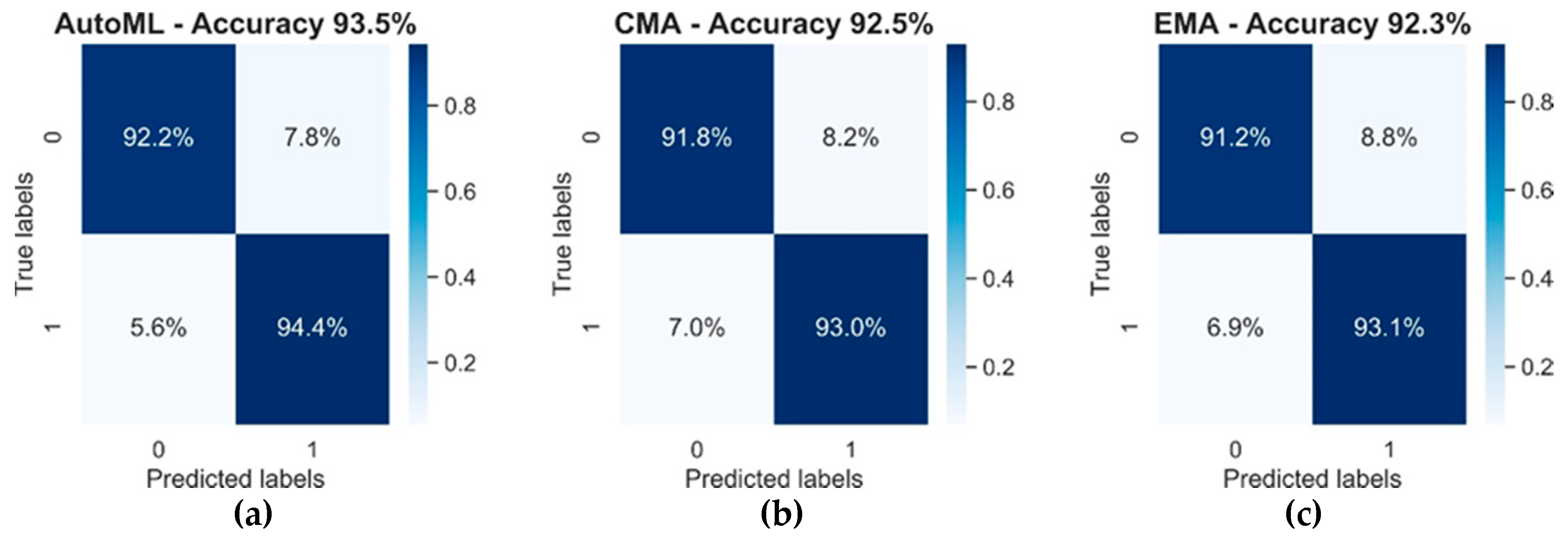
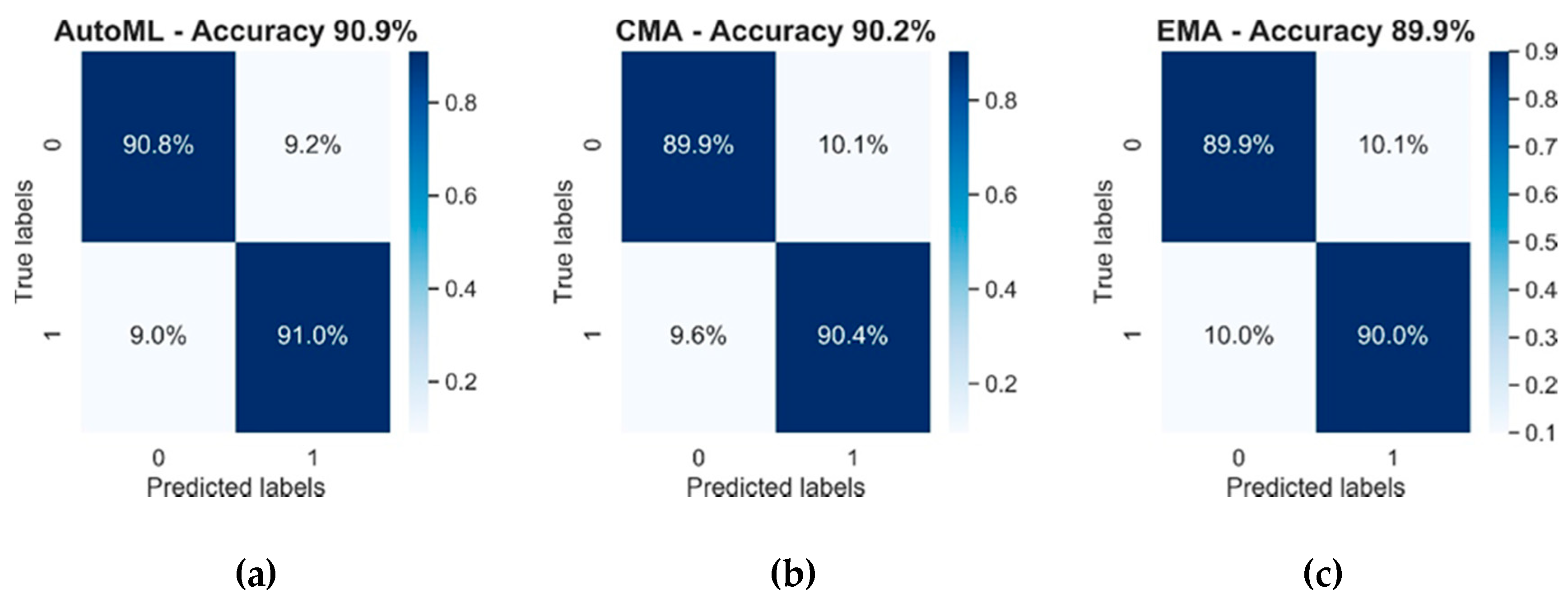
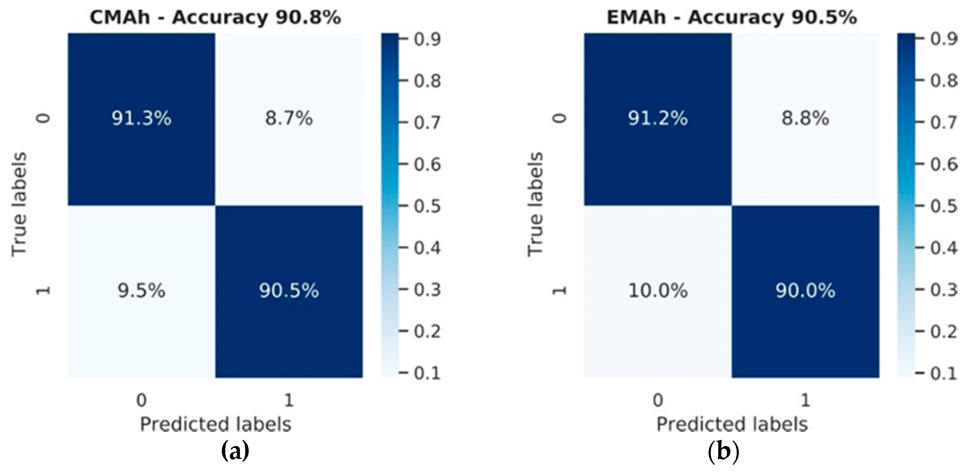
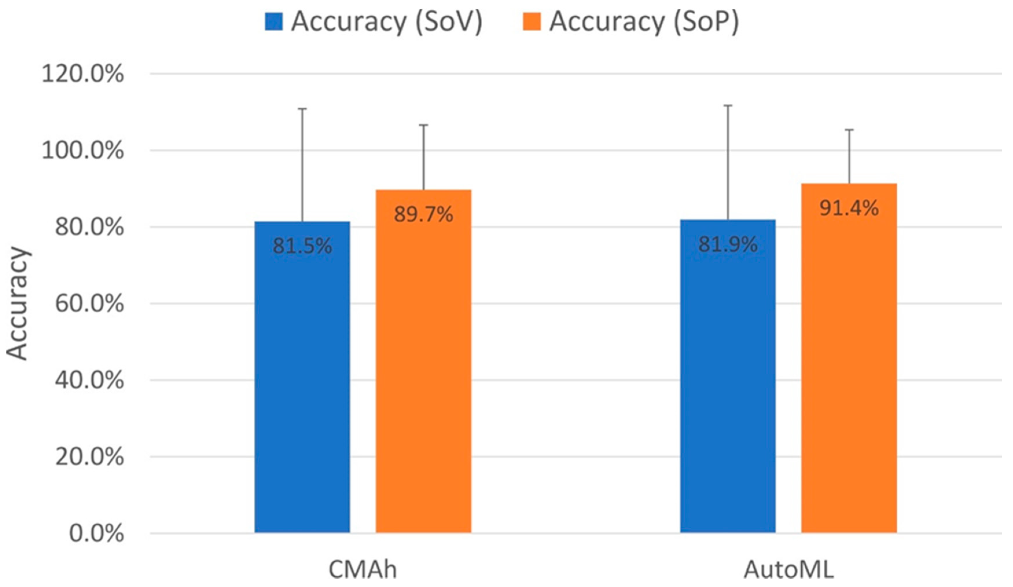
In this section, comparative results are presented for the three models during training and on the test dataset. The underlying cause of differences in these results was analysed, and modifications were made to the averaging approaches to account for these differences. The ability of the models to predict availability on a vehicle-by-vehicle basis was then assessed, and a metric was developed to identify vehicles that were good candidates for V2G. Results for cumulative, fleet-level prediction were also presented. The section concludes with a detailed discussion.

3.1. Model Analysis

The training dataset was used to train models using each of the three approaches. Figure 1 shows the confusion matrices and accuracies, following training on the 34-week training dataset. All three models produced similar accuracies with AutoML, achieving a small increase in accuracy over the two averaging approaches. All the models showed a slightly increased propensity for misclassifying periods the vehicle was not available (true label=0) as periods the vehicle was available (predicted label=1), as shown in the upper right quadrants of the confusion matrices.
To determine if this performance carried over to novel data, the models were tested against the 8-week test dataset. The results in Figure 2 showed that although the accuracy of all 3 models reduced on the test set, the performance remained relatively robust with an accuracy of approximately 90% in all cases. A McNemar test [26] was performed to test the statistical significance between each of the models. The difference between all models was found to be highly significant (p < 0.001). This indicated that although the overall accuracy was similar for all models, the set of classification errors made by each approach was significantly different.
To further explore the differences between the models, accuracy was calculated for University term and non-term periods and separately for holidays and non-holidays. Figure 3 shows that performance for term and non-term periods was very similar for all models, including the averaging approaches for which term was not considered during training. This suggested that fleet behaviour was not substantially impacted by this feature. This was not the case, however, for holidays for which the averaging approaches performed poorly and AutoML very well.
To demonstrate the reasons for this disparity, the average available vehicles for each half-hour period during the two holidays on Mondays in the test dataset was compared to that predicted by each of the three models. Figure 4 shows that the actual availability was relatively static throughout the holidays, a pattern that was typical for a weekend. AutoML correctly identified this pattern; however, the predictions for both CMA and EMA were representative of a typical non-holiday Monday. This was as would be expected, given that the holiday feature was not considered in those approaches.
To accommodate this prediction error, a heuristic was used for the CMA and EMA models that treated any holiday as a Sunday. Therefore, for any rows in the test set with hol = 1, the prediction for Sunday was used, i.e., d was set to 0 for that row. The revised models, termed CMAh and EMAh, were tested on the same 8 weeks training set using this heuristic and the revised confusion matrices and accuracies, as shown in Figure 5.
The accuracy of both averaging approaches increased through the use of the holiday heuristic and was now comparable to AutoML. A McNemar test was performed and again showed a highly significant difference between the averaging models and the AutoML model (p < 0.001). However, no significant difference was now found between the CMAh and EMAh models (p > 0.05).

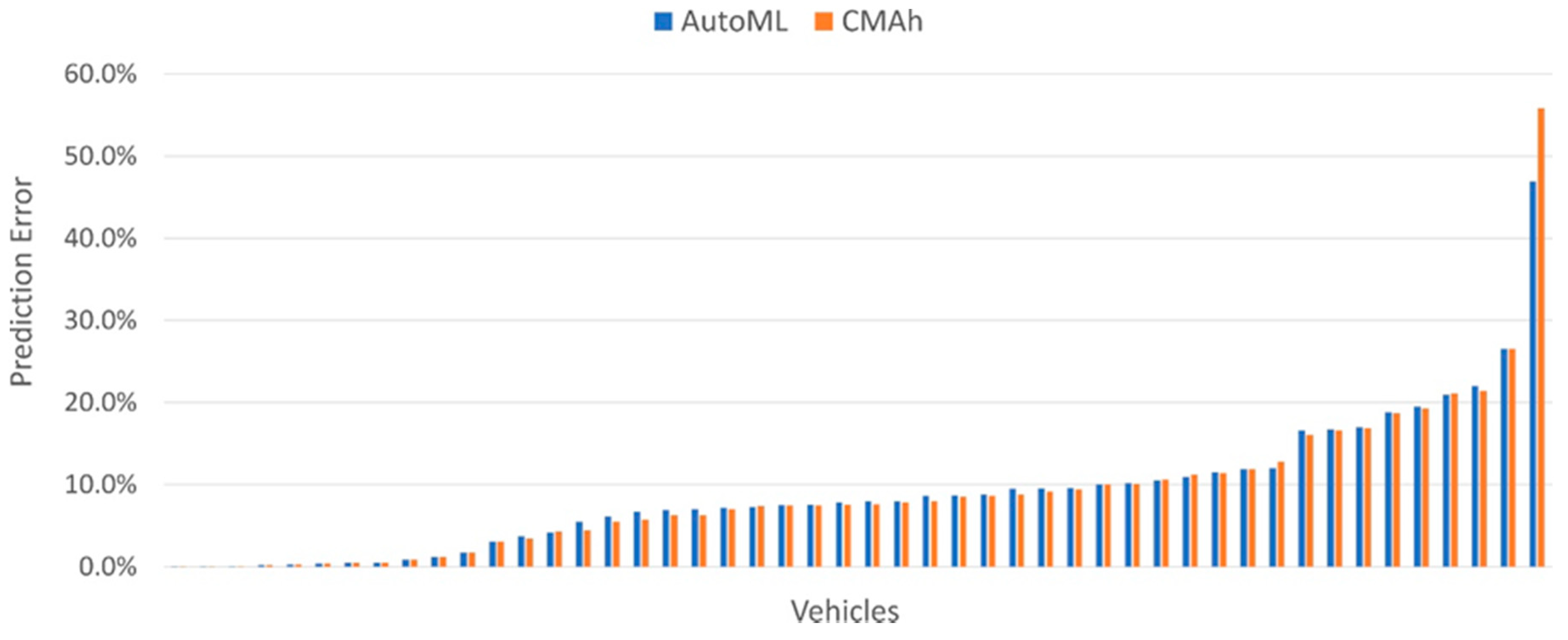
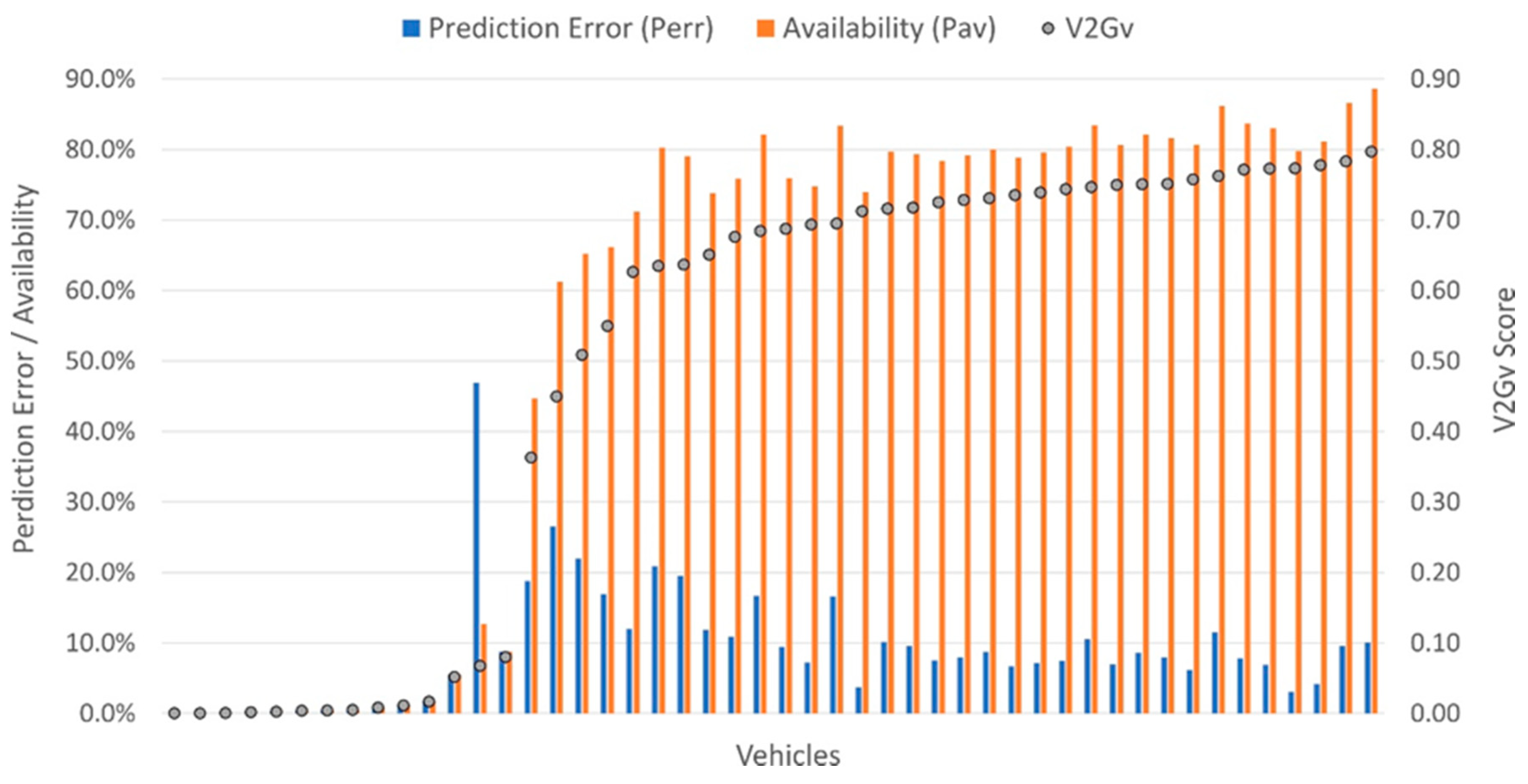
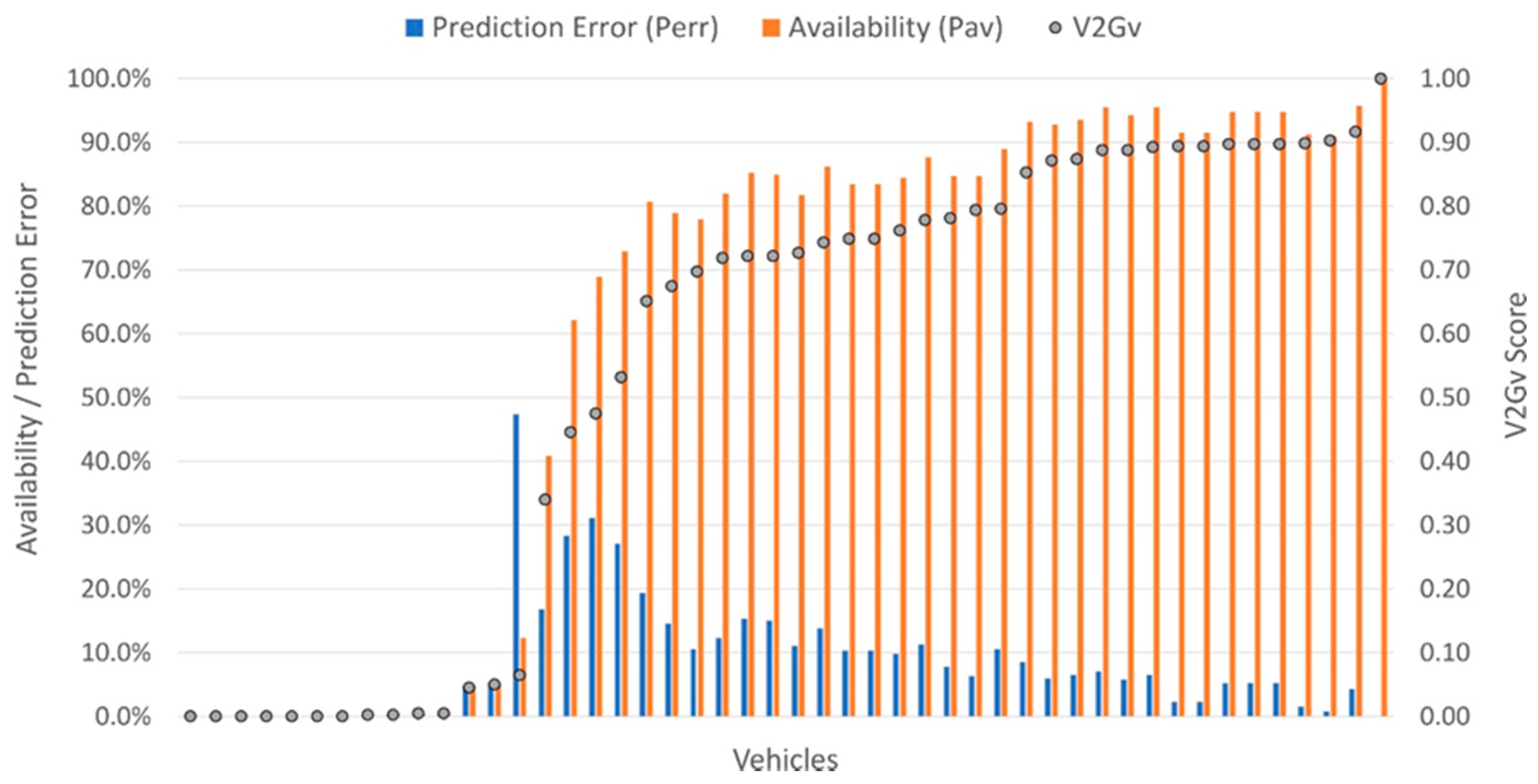
3.2. Vehicle Analysis

To help better understand the performance of the models, the results for each individual vehicle were analysed. Prediction errors for each of the 48 vehicles were determined by calculating the proportion of the test dataset for which the predicted availability was incorrect for that vehicle. Given that the results from the two averaging approaches were not significantly different, the results were only reported for one of the two models (CMAh) for purposes of clarity.
Figure 6 reveals a high degree of correlation between the two models and a clear outlier with a much higher error rate than other vehicles. The analysis of the datasets revealed that was due to a substantially different pattern of behaviour in the 8 test weeks to the 34 training weeks. The vehicle was available for 50.1% of the training period in contrast to only 12.7% of the test period. A similar, but smaller, disparity between training data and test data was also apparent for the two next worse performers. However, this was not always the case for vehicles with a relatively high prediction error. There was a close correlation between the proportion of available periods in the training and test data for the vehicle with the 4th highest error rate despite a prediction error in excess of 20%. In this case, the error was more strongly influenced by the specific times the vehicle was available rather than the total time it was available.
At the other extreme, the figure showed 11 vehicles with error rates of less than 2%. However, the analysis revealed that this excellent performance was enabled by the fact they were almost always unavailable. As a result, both models predicted that these vehicles were never available, and the error rate was due to the small number of periods where this wasn’t the case. Such vehicles would not be appropriate for V2G as they must be both relatively predictable and available for substantial amounts of time. A simple metric was thus developed to calculate the viability of a vehicle, given these variables, as shown in Equation (5), where P e r r is the prediction error, and P a v   the percentage of time the vehicle was available, both expressed as a number between 0 and 1.
V 2 G v = ( 1 P e r r ) P a v
Thus, a stationary vehicle that was entirely predictable and always available would score 1. A vehicle that was either entirely unpredictable and/or never available would score 0, and potentially viable vehicles would score somewhere in between. Figure 7 shows this metric calculated for all vehicles using the test dataset and prediction errors from the AutoML model.
The figure suggested which vehicles would be candidates for V2G. For example, 30 of the 48 vehicles had a V2Gv score in excess of 0.6 as a result of a combination of relatively low prediction errors and relatively high availability. The same set of 30 vehicles was produced using all three models and consisted of vehicles from every department. Of particular interest for a V2G service, however, is the ability to deliver grid services when most required, i.e., at time of peak demand. To determine whether this was the case, the analysis was repeated, considering only periods within a typical peak demand period of 16:00 to 19:00. Figure 8 shows that 30 vehicles again achieved a V2Gv score over 0.6, with only 1 vehicle differing from the original set. However, 15 vehicles now scored over 0.85, making them excellent candidates for participation in V2G during peak hours.
Such a score is not in itself sufficient to demonstrate the viability of a vehicle for V2G however. Another key consideration is the ability of the vehicle to deliver the required power or energy when called upon, i.e., it must have sufficient charge to satisfy journey requirements while delivering energy for the V2G service. To assess this requirement, vehicle trip journey over the 34 weeks of training data was analysed to determine the mean daily mileage for each vehicle on a workday and non-workday. This gave an indication of how much battery capacity would be required to satisfy typical journey requirements and hence how much would be available for V2G. The mean workday daily mileage for vehicles with a peak period V2Gv score over 0.6 was found to be only 26 km (s = 21.8 km), and they were rarely used on other days. It would, therefore, be possible to satisfy these journey requirements while enabling V2G with relatively modest battery capacity. In addition, the vehicles were available on average 96.9% (s = 3.9%) of the time, during the hours of 7 pm and 7 am, thus providing the opportunity for them to start the working day fully charged.

3.3. Fleet Analysis

The vehicle analysis presented in the previous section was of value in assessing the viability of individual vehicles for V2G; however, in order to participate in grid services, the pooled available capacity is likely to be of principal concern to an aggregator. One key requirement for predicting this capacity is predicting the total number of vehicles available at a future time, i.e., it may not be necessary to predict the availability of individual vehicles if the total number available can be predicted. Two approaches were used to make this prediction: a sum of individual vehicle’s predicted binary availability (SoV) and a sum of individual vehicle’s probability of availability (SoP).
To calculate SoV, the binary availability of each vehicle ( a v ) predicted by the model ( m ) for a unique half-hour period ( h h u ) in the test dataset was summed, i.e., t o t a l a v ( m ,   h h u ) = v = 1 n a v ( m , h h u ) . The actual number of available vehicles for a period h h u in the test set was also determined. An error score,   e r r o r ( m ) , was then calculated for the model m by averaging the percentage error between actual and predicted total availability over all 2736 (57 days * 48) unique half-hour periods in the test dataset. The accuracy of the model was defined as a c c u r a c y ( m ) = 1     e r r o r ( m ) .
The SoP approach was identical to the SoV approach with the exception that the total availability predicted by the model m for half-hour period h h u was calculated by summing the predicted probability of each vehicle being available, i.e., a threshold was not used to make a binary prediction for each vehicle before summing. For example, given four vehicles, each with a probability of 0.25 that would individually be predicted to be unavailable, this method would predict one vehicle of the group to be available. In this way, vehicles always contributed to the predicted total in correlation with their likelihood of availability.
These calculations were performed for the CMAh and AutoML models. The results, shown in Figure 9, revealed that the accuracy for both models was relatively low using the SoV approach, and no significant difference was found between the two models using a Welch’s t-test (p > 0.05). However, the use of the SoP approach improved accuracy by 8.2% for CMAh and 9.5% for AutoML, both of which were found to be highly statistically significant improvements (p < 0.001). The accuracy of AutoML-SoV was 1.7% higher than that of CMAh-SoV, a result that was also highly statistically significant (p < 0.001).

3.4. Discussion

The learning approaches explored in this work ranged from the simplest averaging techniques to complex machine learning models. However, their performance on the defined task was comparable. This relative equality could be explained by examining the nature of the dataset and the potential patterns of vehicle behaviour that the machine learning approaches had the potential to learn. A University tends to work on annual patterns as it moves through the various terms and holidays. However, as the training set was exclusively drawn from a single year, any annual patterns could not be learned by the machine learning models. This left two other key features that could potentially be utilised, term and holiday. The CMA and EMA averaging techniques did not consider the term, and yet their performance was equivalent during both periods, and thus this feature had little impact on overall vehicle behaviour. In contrast, the holiday feature did impact vehicle behaviour, which was successfully learned by the AutoML model, resulting in improved performance over the averaging techniques. However, the impact was clear and consistent, and, therefore, a simple heuristic was sufficient to compensate for it within the CMA and EMA models.
There was little scope, therefore, for the machine learning approaches to improve over the simple averaging techniques. This, however, would not always be the case. There are many other features that have the potential to impact vehicle behaviour. For the University fleet, these include University open days, special events, weather events and local traffic conditions. Creation of a successful predictive model for vehicle availability is thus not likely to be a one-off event but rather an iterative process where initially available data is used to produce a first model iteration that is retrained and updated as new data becomes available and its performance analysed. For example, observation of periods of significant deviation between actual and predicted availability may allow the identification of events that need to be accommodated within the model. For the examples above, new features may be added to the dataset to identify open days and special events, allowing any associated impact on vehicle behaviour to be learned. Links to live weather and traffic services may also be established so that the impact of various conditions can be accommodated in the data and influence the predictions that are made. As the complexity of the feature set grows and these features interact non-linearly, the impact of individual features will be less easily identifiable, and, therefore, attempting to accommodate them through use of heuristics in the averaging approaches will quickly become untenable. Machine learning approaches can more easily accommodate such complexity and are, therefore, likely to outperform the averaging approaches as a V2G service develops. However, this will require defining the features that have an impact on vehicle predictability and discovering where the relevant data can be found (e.g., labelling of workplace-specific holidays may require parsing events from work calendars, manual input from fleet owners, etc.).
The need to continually iterate and refine the models is also required to enable adaptation to changes in vehicle behaviour. Although the behaviour of the fleet considered in this work was relatively regular, changes would occur over time in response to changes in the way the broader organisation operates, for example. Such changes in schedule would also be apparent for non-fleet users, where they might be more pronounced given that there is likely to be greater flexibility in drivers’ schedules. The EMA model used in this work weighted recent data more strongly than historical data to help adapt to changes. However, online or continual learning would also be required for machine learning models to adapt to such concept drift [27].
Analysis of individual vehicles allowed the identification of candidate vehicles for V2G. A “sweet spot” of vehicles was identified that satisfied several enabling requirements: (a) they were available, i.e., parked next to a charge point for a significant amount of time; (b) they were predictable, i.e., errors were low; (c) average daily mileage requirements were relatively low, thus providing spare capacity; (d) they were stationary for at least one extended period, thus allowing the battery to be replenished. Such analysis is of value to a fleet that is considering moving to electric vehicles and the use of V2G services by supporting the prioritisation of vehicles to transition and informing the required capacity of batteries, for example. It is also of importance to assess the number of charge points that are required in each proposed location; even if parked locations can be reliably predicted, this is of little value if all the vehicles cannot find a compatible grid connection. Knowledge of individual vehicles is also important during the operation of a V2G service. It may not be possible to assume the use of a vehicle even if it is plugged in and available as it may be necessary for individuals to receive and accept offers to participate in a given V2G opportunity [28], an issue that may be particularly pertinent for non-fleet users. For non-homogeneous populations of vehicles and batteries, it may also be necessary to target users based on the specific capabilities of their vehicles, such as battery capacity. Such socio-technical considerations have not been widely considered in work to date [29], and more research is required.
In many cases, it will be more beneficial to consider the population of available vehicles rather than individual vehicles. The analysis conducted in this paper showed that considering the cumulative likelihood of vehicle availability was more accurate than making predictions for each vehicle individually, which was especially the case for AutoML. To participate in grid services, the most important thing an aggregator needs to predict is the total capacity available to it at a given time, and the specific vehicles contributing to that capacity may be of lesser concern. However, there are a number of other factors that must be considered when translating vehicle availability to actual available capacity. Chief among these is the battery state of charge, which must be sufficient to enable V2G services while allowing a vehicle to continue operating in its primary role as a form of transport. In this work, the average daily mileage was calculated, which allowed likely available surplus capacity to be assessed for given battery capacity. Such high-level analysis may broadly enable a V2G service; however, more detailed analysis of the historical state of charge and incorporation of such data into the learning algorithm would be of great value to optimise the service. This is particularly true for vehicle populations with larger or less consistent daily mileage, where the explicit state of charge data may be essential to calculating whether a vehicle can participate in a V2G event while retaining enough charge for its next journey. As V2G services develop, such data will be generated as vehicles plug into compatible charge points, which can be used to further refine the models and enable finer-grained capacity predictions.

4. Conclusions

In this work, we compared the use of automated machine learning and moving averages to predict the parked locations of vehicles from a University fleet and their proximity to six proposed sites of V2G charging stations. This allowed the potential availability of vehicles during future half-hour trading periods to be assessed. Prediction errors for individual vehicles were found to be very similar for the simplest averaging techniques and the most complex machine learning techniques. However, this was only enabled using a heuristic for the averaging approaches to adjust for the impact of a key feature in the dataset. This impact was learned without intervention by the AutoML approach, a capability that is of critical importance as the feature set grows and interacts non-linearly making the use of heuristics untenable. Two approaches for using the predictions for individual vehicles to predict the total number of available vehicles were also investigated. It was found that calculating the cumulative probability was more powerful than summing individual vehicle predictions and that AutoML was the most accurate using this approach with an accuracy of 91.4% on the test dataset. While this predictive capability would be of value to a V2G aggregation service, translating available vehicles to available capacity requires the incorporation of other factors, including the state of charge of the battery, which will be a focus of future work.

Author Contributions

Conceptualization, R.S., S.N. and J.P.; data curation, R.S., J.W. and L.R.; formal analysis, R.S.; funding acquisition, R.S. and M.G.; investigation, R.S.; methodology, R.S.; software, R.S.; validation, R.S.; writing—original draft, R.S.; writing—review and editing, J.W., S.N. and J.P. All authors have read and agreed to the published version of the manuscript.

Funding

This research and the APC were funded by the European Space Agency, grant number 4000120818/17/NL/US.

Acknowledgments

This work is part of a collaborative project with our partners Kearney, Brixworth Technologies and Cenex—the centre of excellence for low carbon and fuel cell technologies.

Conflicts of Interest

The authors declare no conflict of interest.

References

  1. Villar, J.; Bessa, R.; Matos, M. Flexibility products and markets: Literature review. Electr. Power Syst. Res. 2018, 154, 329–340. [Google Scholar] [CrossRef]
  2. Waldron, J.; Rodrigues, L.; Gillott, M.; Naylor, S.; Shipman, R. Towards an electric revolution: a review on vehicle- to-grid, smart charging and user behaviour. In Proceedings of the 18th International Conference on Sustainable Energy Technologies (SET 2019), Kuala Lumpur, Malaysia, 20–22 August 2019; Volume 3, pp. 1–9. [Google Scholar]
  3. Kempton, W.; Tomić, J. Vehicle-to-grid power implementation: From stabilizing the grid to supporting large-scale renewable energy. J. Power Sources 2005, 144, 280–294. [Google Scholar] [CrossRef]
  4. Nottingham City Council. Nottingham’s 2028 Carbon Neutral Charter; 2019. Available online: http://documents.nottinghamcity.gov.uk/download/7536 (accessed on 14 April 2020).
  5. Pudjianto, D.; Ramsay, C.; Strbac, G. Virtual power plant and system integration of distributed energy resources. IET Renew. Power Gener. 2007, 1, 10. [Google Scholar] [CrossRef]
  6. Nuvve V2G Technology. Available online: https://nuvve.com/technology/ (accessed on 27 February 2020).
  7. Payne, G. Understanding the True Value of V2G; Cenex: Loughborough, UK, 2019; p. 62. Available online: https://www.cenex.co.uk/app/uploads/2019/10/True-Value-of-V2G-Report.pdf (accessed on 14 April 2020).
  8. Powerloop V2G. Available online: https://www.octopusev.com/powerloop (accessed on 27 February 2020).
  9. OVO Vehicle-to-Grid Charger. Available online: https://www.ovoenergy.com/electric-cars/vehicle-to-grid-charger (accessed on 27 February 2020).
  10. Bates, J.; Leibling, D. Spaced Out Perspectives on Parking Policy; RAC Foundation: London, UK, 2012; p. 118. Available online: https://www.racfoundation.org/assets/rac_foundation/content/downloadables/spaced_out-bates_leibling-jul12.pdf (accessed on 14 April 2020).
  11. Zhou, Y.; Cao, S.; Hensen, J.L.M.; Lund, P.D. Energy integration and interaction between buildings and vehicles: A state-of-the-art review. Renew. Sustain. Energy Rev. 2019, 114, 109337. [Google Scholar] [CrossRef]
  12. Iversen, E.B.; Morales, J.M.; Madsen, H. Optimal charging of an electric vehicle using a Markov decision process. Appl. Energy 2014, 123, 1–12. [Google Scholar] [CrossRef] [Green Version]
  13. Shimizu, O.; Kawashima, A.; Inagaki, S.; Suzuki, T. Vehicle Fleet Prediction for V2G System - Based on Left to Right Markov Model. In Proceedings of the 4th International Conference on Vehicle Technology and Intelligent Transport Systems, Madeira, Portugal, 16–18 March 2018; pp. 417–422. [Google Scholar]
  14. Hou, Y.; Edara, P. Network Scale Travel Time Prediction using Deep Learning. Transp. Res. Rec. 2018, 2672, 115–123. [Google Scholar] [CrossRef]
  15. Awan, F.M.; Saleem, Y.; Minerva, R.; Crespi, N. A Comparative Analysis of Machine/Deep Learning Models for Parking Space Availability Prediction. Sensors 2020, 20, 322. [Google Scholar] [CrossRef] [PubMed] [Green Version]
  16. Trakm8 Limited. Telematic Solutions. 2019. Available online: https://static.trakm8.com/static/downloads/trakm8-telematics-solutions-brochure.pdf (accessed on 14 April 2020).
  17. Hutter, F.; Kotthoff, L.; Vanschoren, J. Automated Machine Learning, 1st ed.; Springer International Publishing: New York, NY, USA, 2019; p. 242. ISBN 9783030053178. [Google Scholar]
  18. Waldron, J.; Rodrigues, L.; Gillott, M.; Naylor, S.; Shipman, R. Decarbonising Our Transport System: User Behaviour Analysis to Assess the Transition to Electric Mobility. In Proceedings of the 35th PLEA conference sustainable architecture and urban design (to appear), A Coruña, Spain, 1–3 September 2020. [Google Scholar]
  19. Fusi, N.; Sheth, R.; Elibol, M. Probabilistic matrix factorization for automated machine learning. In Proceedings of the 32nd Conference on Neural Information Processing Systems (NeurIPS 2018), Montréal, Canada, 3–8 December 2018; pp. 3348–3357. [Google Scholar]
  20. Feurer, M.; Klein, A.; Eggensperger, K.; Springenberg, J.; Blum, M.; Hutter, F. Efficient and Robust Automated Machine Learning. In Advances in Neural Information Processing Systems, 28th ed.; Cortes, C., Lawrence, N.D., Lee, D.D., Sugiyama, M., Garnett, R., Eds.; Curran Associates, Inc.: New York, NY, USA, 2015; pp. 2962–2970. [Google Scholar]
  21. Microsoft Corporation. What is Automated Machine Learning? Available online: https://docs.microsoft.com/en-us/azure/machine-learning/concept-automated-ml (accessed on 28 February 2020).
  22. Chen, T.; Guestrin, C. XGBoost: A scalable tree boosting system. In Proceedings of the 22nd ACM SIGKDD International Conference on Knowledge Discovery and Data Mining, San Francisco, CA, USA, 13–17 August 2016; pp. 785–794. [Google Scholar]
  23. Google AutoML Tables. Available online: https://cloud.google.com/automl-tables (accessed on 6 February 2020).
  24. Zoph, B.; Le, Q.V. Neural architecture search with reinforcement learning. In Proceedings of the 5th International Conference on Learning Representations ICLR 2017, Toulon, France, 24–26 April 2017; pp. 1–6. [Google Scholar]
  25. Cortes, C.; Gonzalvo, X.; Kuznetsov, V.; Mohri, M.; Yang, S. AdaNet: Adaptive Structural Learning of Artificial Neural Networks. In Proceedings of the 34th International Conference on Machine Learning, Sydney, Australia, 6–11 August 2017; Volume 70, pp. 874–883. [Google Scholar]
  26. Dietterich, T.G. Approximate Statistical Tests for Comparing Supervised Classification Learning Algorithms. Neural Comput. 1998, 10, 1895–1923. [Google Scholar] [CrossRef] [PubMed] [Green Version]
  27. Gama, J.; Žliobaitundefined, I.; Bifet, A.; Pechenizkiy, M.; Bouchachia, A. A Survey on Concept Drift Adaptation. ACM Comput. Surv. 2014, 46, 1–37. [Google Scholar] [CrossRef]
  28. Shipman, R.; Naylor, S.; Pinchin, J.; Gough, R.; Gillott, M. Learning capacity: predicting user decisions for vehicle-to-grid services. Energy Informatics 2019, 2, 1–22. [Google Scholar] [CrossRef] [Green Version]
  29. Sovacool, B.K.; Noel, L.; Axsen, J.; Kempton, W. The neglected social dimensions to a vehicle-to-grid (V2G) transition: a critical and systematic review. Environ. Res. Lett. 2018, 13, 13001. [Google Scholar] [CrossRef]
Figure 1. Confusion matrices and accuracy of all 3 models on the training dataset. The labels indicate predicted and actual vehicle availability. AutoML, automated machine learning (a); CMA, cumulative moving average (b); EMA, exponential moving average (c).
Energies 13 01933 g001
Figure 2. Confusion matrices and accuracies of the 3 models on the test dataset. The labels indicate predicted and actual vehicle availability. AutoML, automated machine learning (a); CMA, cumulative moving average (b); EMA, exponential moving average (c).
Energies 13 01933 g002
Figure 3. Accuracy of the 3 models for term/non-term periods and holiday/workdays. Data labels show accuracy for holidays.
Energies 13 01933 g003
Figure 4. Total available vehicles predicted by the 3 models for the 2 holiday Mondays in the test dataset compared to actual availability.
Energies 13 01933 g004
Figure 5. Confusion matrices and accuracies for the averaging approaches using the holiday heuristic. CMAh, cumulative moving average with holiday heuristic (a); EMAh, exponential moving average with holiday heuristic (b).
Energies 13 01933 g005
Figure 6. Prediction errors (Perr) for each of the 48 vehicles for the AutoML and CMAh models.
Energies 13 01933 g006
Figure 7. V2G (vehicle-to-grid) viability scores, V2Gv, for the 48 fleet vehicles using the AutoML model on the test dataset.
Energies 13 01933 g007
Figure 8. V2Gv scores for the peak 4 pm to 7 pm period using the AutoML model on the test dataset.
Energies 13 01933 g008
Figure 9. Accuracy of the predicted total number of vehicles over the test period using 2 different approaches (SoV and SoP) for the CMAh and AutoML models (see text for details). Error bars show +1 standard deviation. SoV, the sum of individual vehicle’s predicted binary availability; SoP, the sum of individual vehicle’s probability of availability.
Energies 13 01933 g009
Table 1. Example data received for each vehicle journey.
NameDescriptionExample
vidUnique identifier for this vehicle12
start_latLatitude at the start of the journey52.95282
start_lngLongitude at the start of the journey−1.18652
start_timeTimestamp at the start of the journey2019-11-21T13:53:10+00:00
end_latLatitude at the end of the journey52.94025
end_lngLongitude at the end of the journey−1.192132
end_timeTimestamp at the end of the journey2019-11-21T14:00:16+00:00
Table 2. Sample data from the processed dataset.
Vehicle (v)Departmentdhhphuhholtermav
1A1101100
2B33500011
3C52610100
3C52710101
4D42000011
Where d = day; hh = half-hour period; ph=public holiday; uh = university holiday; hol = holidays; term = university term and av = vehicle availability.
Table 3. Composition of the training and test datasets.
FeatureTrainingTest
Availability (av = 1)57.4%55.7%
Term days (term = 1)54.4% (129 days)47.4% (27 days)
Public Holiday (ph = 1)3.0% (7 days)1.8% (1 day)
University Holiday (uh = 1)1.7% (1 day)1.8% (1 day)

