Article

The Impact of Imperfect Weather Forecasts on Wind Power Forecasting Performance: Evidence from Two Wind Farms in Greece

by
Evangelos Spiliotis
1,†,
Fotios Petropoulos
2,*,† and
Konstantinos Nikolopoulos
3,†
1
Forecasting and Strategy Unit, School of Electrical and Computer Engineering, National Technical University of Athens, 15780 Athens, Greece
2
School of Management, University of Bath, Bath BA2 7AY, UK
3
ForLAB, Bangor Business School, Bangor University, Bangor LL57 2DG, UK
*
Author to whom correspondence should be addressed.
These authors contributed equally to this work.
Energies 2020, 13(8), 1880; https://doi.org/10.3390/en13081880
Submission received: 11 March 2020 / Revised: 27 March 2020 / Accepted: 3 April 2020 / Published: 12 April 2020

Abstract

:
Weather variables are an important driver of power generation from renewable energy sources. However, accurately predicting such variables is a challenging task, which has a significant impact on the accuracy of the power generation forecasts. In this study, we explore the impact of imperfect weather forecasts on two classes of forecasting methods (statistical and machine learning) for the case of wind power generation. We perform a stress test analysis to measure the robustness of different methods on the imperfect weather input, focusing on both the point forecasts and the 95% prediction intervals. The results indicate that different methods should be considered according to the uncertainty characterizing the weather forecasts.

1. Introduction

Forecasts are an integral part of the decision-making process. They can take the form of judgmental, human-made forecasts or statistical, machine-made, formal forecasts. Forecasts are used at different levels of decision-making, from the very granular, operational level to the very aggregate, strategic level. The most common form of forecasting is a set of point forecasts (most likely estimates). However, the efficient estimation of uncertainty, in the form of prediction intervals or probabilistic/density forecasts, is also crucial [1]. This is especially true when one deals with highly volatile environments. While oftentimes univariate time series forecasting techniques are appropriate for making extrapolations, in some instances, the observed past patterns are not the best predictor for the future, with the dependent variable being affected by external, independent factors. In such cases, regression-like forecasts are required.
When using independent variables (predictor or exogenous variables) to forecast the dependent, target variable of interest, one common challenge is related with the accuracy of the future values of these predictors. In some settings, this might be trivial to tackle. For instance, if promotional indicators are used to produce demand forecasts, then information regarding future promotions should be (at least internally) readily available. However, when predictors such as gross domestic product or unemployment are used to predict demand, then one needs to accurately extrapolate these independent variables before producing the forecasts for the target variable. An analysis of the results of recent Kaggle forecasting competitions showed that when an independent variable is not trivial to forecast, then its added-value to forecast accuracy is minimal [2].
The increased costs and environmental impacts associated with fossil fuels, combined with the increased global energy demand, led many countries to invest heavily in renewable energy sources. Wind energy is probably the most popular renewable energy source, experiencing an exponential increase in cumulative capacity over the last 25 years, and being rapidly integrated in national energy policies. Wind power forecasting is important to a variety of stakeholders, such as grid system operators, electricity traders, and wind farm operators, with accurate forecasts being crucial for efficient energy storage management [3] and microgrid scheduling [4]. While some researchers suggest bypassing the wind speed forecasts and using direct (univariate) approaches to forecast wind power [5], it is very common for researchers and practitioners alike to use numerical weather predictions (e.g., wind speed and/or direction forecasts) as inputs in their algorithms [6,7,8,9].
However, numerical weather predictions can be inaccurate for several reasons. First, weather stations may be located relatively far from the wind farm [10,11]. As an example, [12] proposed local recurrent neural networks for three-day-ahead wind speed and power forecasting using numerical weather predictions from stations as far away as 30 km. Second, forecasts may be required for further into the future than the short term, making any weather predictions uncertain [12,13]. Third, wind is very volatile in nature, making its prediction difficult [14,15].
Researchers have investigated several techniques to improve wind power forecast through wind speed numerical predictions. Indicatively, these include the use of Kalman filters [16], neural networks [17], and combinations of machine learning (ML) methods [18]. Another example of using imperfect weather forecast towards wind power forecasting is the study by [19], who used wind speed and its standard deviation as inputs to machine learning algorithms. Instead of relying on imperfect meteorological weather predictions, some researchers focused on directly estimating the wind speed using variations of autoregressive integrated moving average models [20,21] or artificial neural networks [22]. However, even in these cases, the wind speed estimates are associated with some volatility (uncertainty), which is also taken into account when estimating the wind power.
In this paper, instead of attempting to correct the biasedness and apply error corrections on the numerical weather predictions, we accept their uncertain nature. Given this uncertainty, we perform a comparison across multiple methods used to forecast wind power in order to understand the effects of weather uncertainty on their forecasting performance. We consider both statistical, linear regression models as well as several nonlinear ML methods [23]. Our research question is as follows: How does weather forecast uncertainty affect the relative performance of statistical and ML methods for wind power forecasting?
Focusing on the case of wind power generation and numerical weather predictions (in terms of wind speed and direction), our contributions are threefold:
  • We measure the impact of imperfect weather forecasts on the wind power forecasting accuracy and the estimation of uncertainty through the evaluation of the point forecasts and the prediction intervals produced by various types of forecasting methods;
  • We compare the suitability of statistical versus ML approaches in the task of estimating highly volatile variables when the accuracy of external information varies;
  • Assuming varying levels of inaccuracy in the independent variable, we perform a sensitivity analysis with varying distributional assumptions to conclude on the robustness [24] of the forecasting approaches considered and make relevant recommendations.
The remainder of the manuscript is organized as follows. Section 2 presents the statistical and ML forecasting approaches used to forecast wind power. Section 3 describes the wind data used in this study, provides the details of the experimental setup, and presents the results. Section 4 discusses the empirical results and provides implications for practice. Section 5 concludes the paper.

2. Forecasting Methods Considered

In this study, we consider seven forecasting methods: a statistical method (Linear Regression, LR) and six ML methods, namely, Multi-Layer Perceptron (MLP), Bayesian Neural Network (BNN), Random Forest (RF), Gradient Boosting Trees (GBT), K-Nearest Neighbor Regression (KNNR), and Support Vector Regression (SVR). The methods were chosen so that the results are representative for the major ML regression algorithms considered in the forecasting literature, i.e., Neural Networks (NNs), Regression Trees (RTs), Support Vector Machines (SVMs), and other nonparametric approaches.

2.1. Training and Testing

The forecasting methods are trained by correlating the wind power (target variable) with the weather forecasts (predictor variable) provided for the same period. Thus, all methods have a single output and as many inputs as the weather variables being forecasted (e.g., wind speed and wind direction). Note that since forecasting is performed through regression, the forecasting horizon and the period at which the forecasts are produced are irrelevant. In other words, the relationships learned are time-independent and used for predicting wind power at any period of interest for which weather forecasts are available.
In order for our results to be more indicative, we implement a fivefold cross-validation procedure which resamples the available data sample and effectively approximates how the considered model is expected to perform when utilized to generate forecasts for periods not used for training [25]. According to this procedure, we first shuffle the dataset randomly and split it into five groups. Then, we use the first four groups for training the method and the last group for testing its performance. We repeat this process for the remaining four combinations of groups and summarize our results by averaging the individual scores.

2.2. Scaling

Given that the majority of the ML methods considered utilize nonlinear activation functions, such as sigmoid ones, the data must be scaled before training so that computational problems are avoided, algorithm requirements are met, and faster learning is facilitated [26]. To that end, we scaled both the target and the predictor variables between 0 to 1 by considering a linear transformation, v , as follows:
v i t = v i t v i min v i max v i min ,
where v i t is the value of the i t h variable of the dataset at point t, and v i min and v i max denote the minimum and maximum value of the variable, respectively, computed for the sample used for training the forecasting methods. The reverse transformation was used to rescale the forecasts derived by the methods so that predictions are expressed in the same scale as that of the wind power.
Given that the major objective of this study was to evaluate the forecasting performance of various methods under conditions of imperfect weather forecasts, which may include extreme, abnormal values, no other types of preprocessing were considered (e.g., trimming and power transformations).

2.3. Statistical and Machine Learning Methods

Below, we summarize the statistical and ML methods used for forecasting wind power, also providing information about the model architectures and hyperparameters used per case.
  • Linear Regression (LR): LR is a linear method for modeling the relationships between the target and the predictor variables. The parameters of the forecasting model are estimated directly from the data using closed forms. LR was the first type of regression method to be studied rigorously, and is therefore widely used because of its simplicity, low computational cost, and intuitiveness. Since in this study we consider N weather variables as predictors, LR is implemented in the form of multiple linear regression, as follows:
    y ^ t = a + b 1 × v 1 + b 2 × v 2 . . . + b k × v k ,
    where a is the intercept of the model, and b j is the coefficient of the j t h weather variable used for predicting the wind power. Note that LR methods, in contrast to ML methods, assume additive, linear relationships between the target and the predictor variables. Thus, it was expected to result in suboptimal forecasts when used for modeling complex, nonlinear data patterns;
  • Multi-Layer Perceptron (MLP): A simple, single hidden layer NN of N input and 2 N input nodes, constructed so that accurate, yet computationally affordable forecasts are provided [27]. The Scaled Conjugate Gradient method is used for estimating the weights [28] which are initialized randomly. The learning rate is selected between 0.1 and 1 using a tenfold cross-validation procedure (mean squared error minimization), while the maximum iterations are set to 500. The sigmoid activation function is used both for the hidden and the output layers given the lack of trend in the data. We trained 10 models and use the median of their forecasts to mitigate possible variations due to poor weight initializations [29]. The method was implemented using the RSNNS R statistical package [30];
  • Bayesian Neural Network (BNN): This method is similar to the MLP method but optimizes the weights according to the Bayesian concept, as suggested by [31,32]. The Nguyen and Widrow algorithm [33] is used to assign initial weights and the Gauss–Newton algorithm to perform the optimization. Once again, an ensemble of 10 models was considered with a maximum of 500 iterations each. The method was implemented using the brnn R statistical package [34];
  • Random Forest (RF): RTs can be used to perform a treelike recursive partitioning of the input space, thus dividing it into regions, called the terminal leaves [35]. Then, on the basis of the inputs provided, tests are applied to decision nodes in order to define which leave should be used for forecasting. The RF method expands this concept by combining the results of multiple RTs, each one depending on the values of a random vector sampled independently and with the same distribution [36]. In this regard, RF is more robust to outliers and overfitting, even for limited samples of data. In this study, we considered a total of 500 nonpruned trees and sampled the data with replacement. The method was implemented using the randomForest R statistical package [37];
  • Gradient Boosting Trees (GBT): This method is similar to RF, but instead of generating multiple independent trees, it builds one tree at a time, each new tree correcting the errors made by the previously trained one [38]. Thus, although GBT is more specialized than RF in forecasting the target variable, is more sensitive to overfitting [39]. In this study, we constructed a slow learning model with a learning rate of 0.01 and a maximum tree depth of 5. We considered 1000 trees but pruned the constructed model by employing a tenfold cross-validation procedure to mitigate overfitting. The method was implemented using the gbm R statistical package [40];
  • K-Nearest Neighbor Regression (KNNR): KNNR is a similarity-based method, generating forecasts according to the Euclidean distance computed between the points used for training and testing. Given a test sample of N predictor variables, the method picks the closest K observations of the training sample to them and then sets the prediction equal to the average of their corresponding target values. K was selected between 3 and 300 with a step of 3 using a tenfold cross-validation procedure. The method was implemented using the caret R statistical package [41];
  • Support Vector Regression (SVR): SVR generates forecasts by identifying the hyperplane that maximizes the margin between two classes and minimizes the total error under tolerance [42]. We considered ϵ -regression, with ϵ being equal to 0.01 and a radial basis kernel. The method was implemented using the e1071 R statistical package [43].

3. Empirical Evaluation
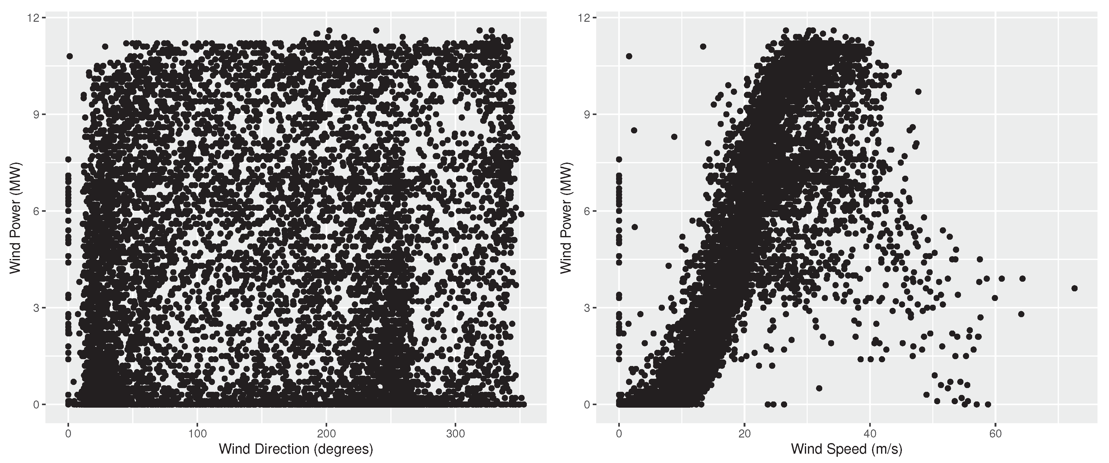
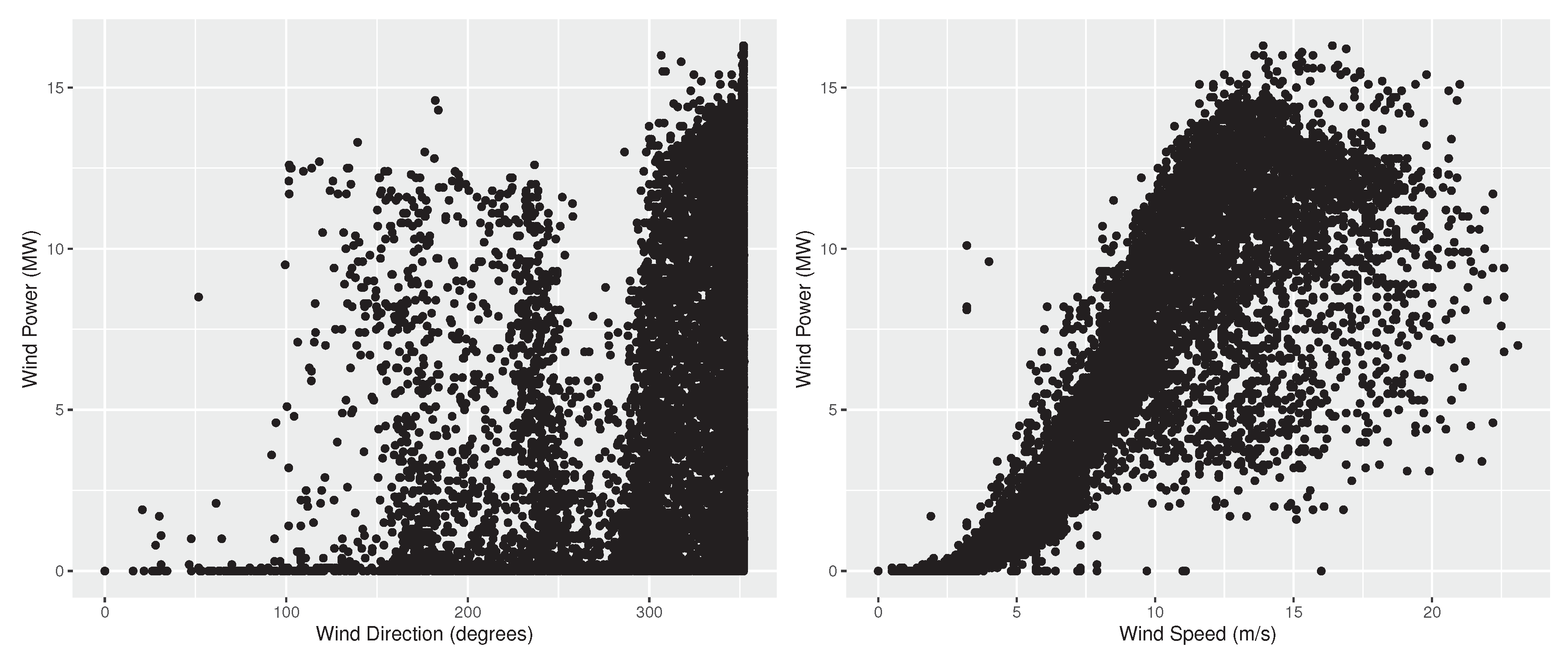
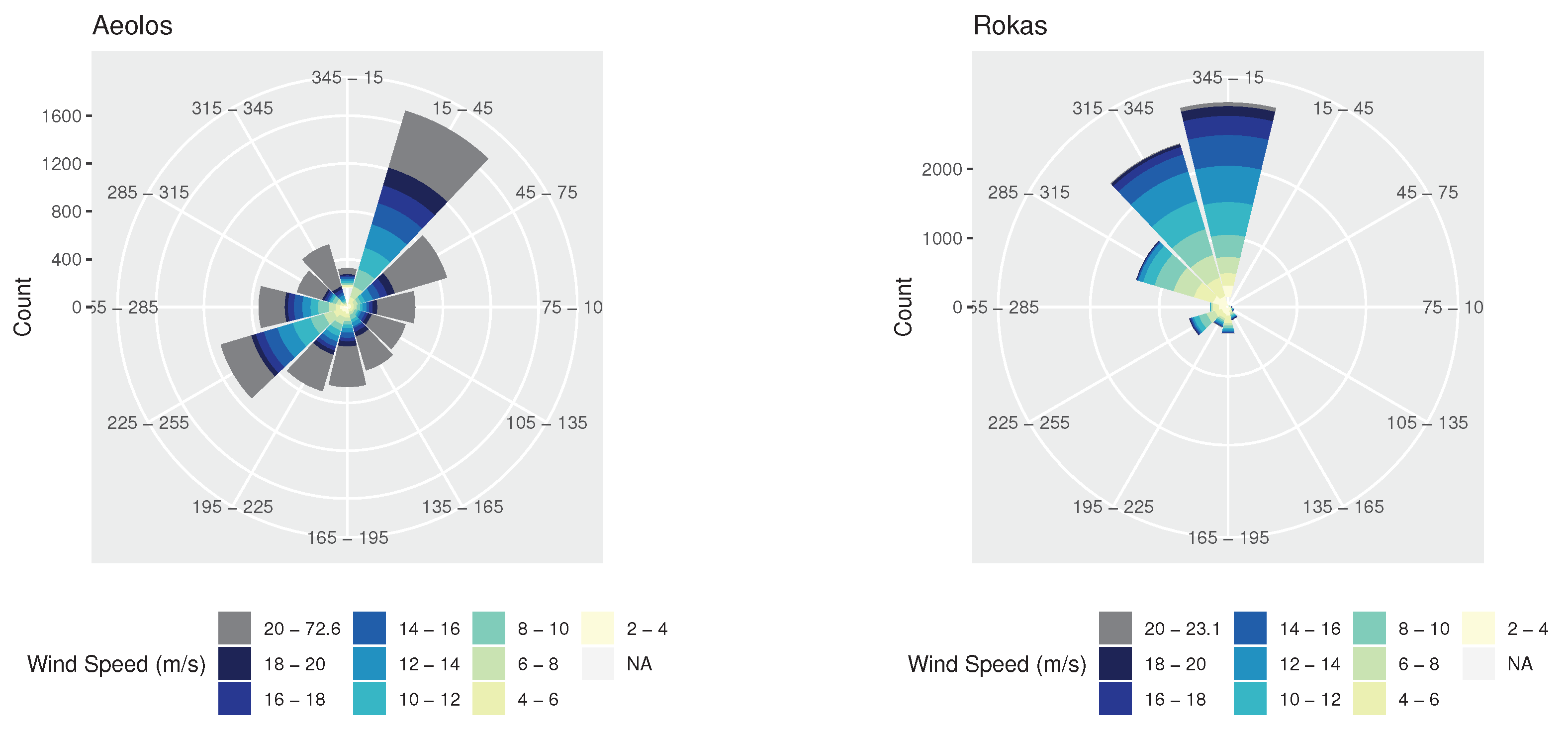
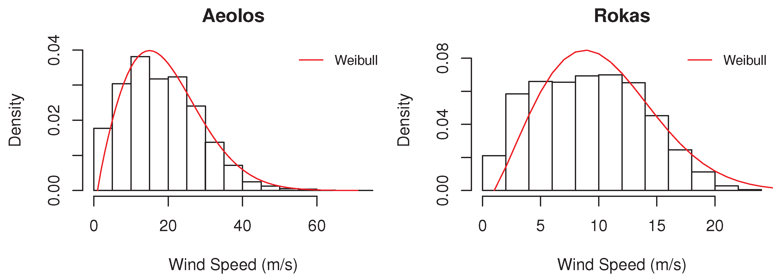
3.1. Dataset

In order to evaluate the impact of imperfect weather forecasts on wind power forecasting performance, we considered two wind farms, namely, Aeolos and Rokas, located in Crete, Greece. The datasets of both wind farms are hourly and have a duration of one year (8760 h) ranging from 1 January 2006 to 31 December 2006. The datasets include the wind speed (measured in m/s) and direction (measured in degrees) recorded at the turbine hub height, as well as the wind power recorded (measured in MW). For more information about the dataset, see [3].
Figure 1 and Figure 2 present the wind power of the two farms versus the wind direction and speed. In practice, the panels of the two figures represent the empirical power curves of the farms, being subject to wind direction and speed, respectively [44]. As seen, in both cases wind power is nonlinearly increased as wind speed becomes larger. Moreover, faster wind is required in the Aeolos wind farm for producing the same power produced in Rokas, where wind speed intensity is typically significantly lower than that of Aeolos. In addition, wind power is more volatile in Rokas than in Aeolos. Observe also that each park is designed so that wind power is maximized for specific wind directions, which are also the most frequently observed ones. In this respect, wind power in Aeolos is maximized for a wind direction of 30 and 240 degrees, while in Rokas for a wind direction of 350 degrees. It is mentioned that wind direction is more volatile in Aeolos than in Rokas, with the latter ranging mainly between 300 and 360 degrees and the former covering all directions. Note also that in both farms, wind power is correlated more strongly to wind speed than to wind direction, meaning that imperfect wind speed forecasts are expected to have a larger impact to wind power forecasting performance. Finally, we should note that in both wind farms there are some cases where wind power is zero or close to zero, although the wind speed is strong. This could be either due to wrong wind speed measurements or a scheduled maintenance.
An overview of how wind speed and direction are distributed at the two wind farms is also provided in the wind roses of Figure 3. As can be seen, in the Aeolos wind farm, wind direction is typically either around 30 or 240 degrees, while in Rokas it is concentrated between 300 and 360 degrees. Moreover, in the Aeolos wind farm, wind speed typically exceeds 18 m/s, in contrast to Rokas where wind speed does not usually exceed 10 m/s. This also becomes evident by observing the Weibull distributions of the wind speed of the two wind farms of Figure 4.

3.2. Experimental Setup

Given that the examined dataset includes two predictor variables, i.e., wind speed and direction, we trained the forecasting methods presented in Section 2 using N = 2 inputs. We split the dataset of each wind farm into five training and test samples (see Section 2.1), scaled the training data (see Section 2.2), and used the trained models to predict the wind power. For every group of the fivefold cross-validation procedure, we recorded the average performance of the forecasting methods and estimated their overall performance by averaging the individual records.
Since forecasting performance is reported for each wind farm separately, we use the mean absolute error (MAE) for measuring the average forecasting accuracy of the examined methods, as follows:
M A E = 1 5 i = 1 5 1 l i j = 1 l i Y i j Y ^ i j ,
where i denotes the number of the cross-validation group, l i is the observations of the test sample of group i, and Y i j and Y ^ i j are the actual and predicted wind power of the jth observation of group i, respectively.
Note that the predictor variables included in the dataset do not represent weather forecasts, but the actual wind speed and direction recorded at the turbine hub height. Thus, using them directly as inputs to the examined forecasting methods is equivalent to predicting wind power under conditions of perfect foresight, i.e., zero uncertainty about the future weather conditions. On the other hand, if the original values of the predictor variables were distorted to some extent, this would be equivalent to predicting wind power under uncertainty, with its level being relative to the extent of the distortion considered.
The aforementioned process can be simulated by injecting noise into the two predictor variables of the dataset. Thus, we built on this concept so that imperfect weather forecasts were created, considering various types of noise, as well as different noise intensities. Without loss of generality, we considered the uniform and the Gaussian noise, given that these types of noise have been considered in past studies for performing similar simulations [45]. In the first case, it was assumed that forecast errors may range anywhere between a lower and an upper limit, while in the second case, we assumed that forecast errors were normally distributed around a mean forecast error, μ , with a standard deviation of σ .
We simulated the weather forecast of normally distributed errors by adjusting the original values of the two predictor variables by a factor which is normally distributed around μ = 1 and μ = 0 for wind speed and direction, respectively, with a standard deviation of σ varying from 0 to 1 with a step of 0.05. Similarly, we simulated the weather forecast of uniformly distributed errors by adjusting the original values of the two predictor variables by a factor which is randomly selected from [1 − s, 1 + s] and [−s, s] for wind speed and direction, respectively, with s varying also from 0 to 1 with a step of 0.05. Essentially, higher values of σ and s indicate higher noise intensity, and as a result, more uncertainty about the future.
Note that in order for the derived forecasts to be meaningful, we customized the simulation performed per weather variable, as follows:
  • Wind speed. Given that wind speed must be positive, the adjustment was performed by (i) multiplying the original values of the variable with the computed factors and (ii) setting all nonzero forecasts (if any) to zero;
  • Wind direction. Given that wind direction must range between 0 and 360 degrees, the adjustment was performed by (i) adding the computed factors, multiplied by 360, to the original values of the variable, and (ii) adding or subtracting 360 to all forecasts that were lower than zero or higher than 360, respectively.
In order to evaluate the impact of imperfect weather forecasts on wind power forecasting performance on a regressor variable level, we considered the following three simulations: (a) noise is injected only to wind direction forecasts; (b) noise is injected only to wind speed forecasts; (c) noise is injected both to wind direction and speed forecasts. This setup allowed us to determine which weather variables are important to be accurately forecasted and if there are any variables for which accurately predicting their future values is irrelevant.
Note that apart from linear regression, which allows for prediction intervals to be computed directly, the rest of the forecasting methods considered do not allow for such theoretical-based approximations [46]. This is due to the nonlinear nature of the ML regression models and the lack of an underlying statistical model [47]. To that end, we considered the bootstrap method, that allows prediction intervals to be empirically, yet precisely estimated [48,49]. The adopted bootstrap approach is summarized as follows:
  • Given the sample used for training the forecasting methods when producing point forecasts, the random samples are created without replacement (observations used for validation purposes remain unobserved while training);
  • For each of the ten random samples, 90% of the observations are used for training the forecasting methods and 10% for estimating the corresponding errors of the point forecasts;
  • The empirical distribution of the errors (actual-forecast) is computed using a Kernel density estimator, and the 0.025 and 0.975 quantities of the distribution are determined;
  • The forecasting methods are retrained using the complete training sample so that point forecasts are produced for the test sample of interest;
  • The 95% prediction intervals are computed by adding the 0.025 and 0.975 quantities to the point forecasts produced in the previous step.
Note that this process is repeated five times, according to the fivefold cross-validation procedure described in Section 2.1. The performance of each of the forecasting methods in terms of prediction intervals is then computed using the Mean Interval Score (MIS) [50], as follows:
M I S = 1 5 i = 1 5 1 l i j = 1 l i U i j L i j + 2 α ( L i j Y i j ) 1 { Y i j < L i j } + 2 α ( Y i j U i j ) 1 { Y i j > U i j } ,
where U i j and L i j are the upper and lower bounds computed for the jth observation of group i, respectively, and a = 0 . 05 (95% confidence). Note that MIS evaluates prediction intervals taking into consideration both their coverage, i.e., the percentage of times when the true values lie inside the prediction intervals, and their spread, i.e., the distance between the upper and lower bounds [51]. Thus, in order for a prediction interval to be effective, it must provide the nominal coverage with the minimum possible width [52].
The experimental setup can be summarized as follows:
  • We randomly split the original dataset of each wind farm into five samples of equal sizes;
  • Four out of the five samples are used for constructing a training dataset, which is then scaled;
  • The training dataset is randomly split into ten subsamples;
  • Nine out of the ten subsamples are used for training the seven forecasting methods considered in this study, with the last one used for producing forecasts and computing the corresponding forecast errors of each method;
  • Step 4 is repeated for all the ten possible combinations of subsamples;
  • A Kernel density estimator is used to approximate the 0.025 and 0.975 quantities of the error distribution of the methods, as specified through Steps 3, 4, and 5;
  • The forecasting models are retrained using the complete training dataset, as specified in Step 2, so that point forecasts are produced for the respective test sample;
  • 95% prediction intervals are computed by adding the 0.025 and 0.975 quantities to the point forecasts produced in Step 7;
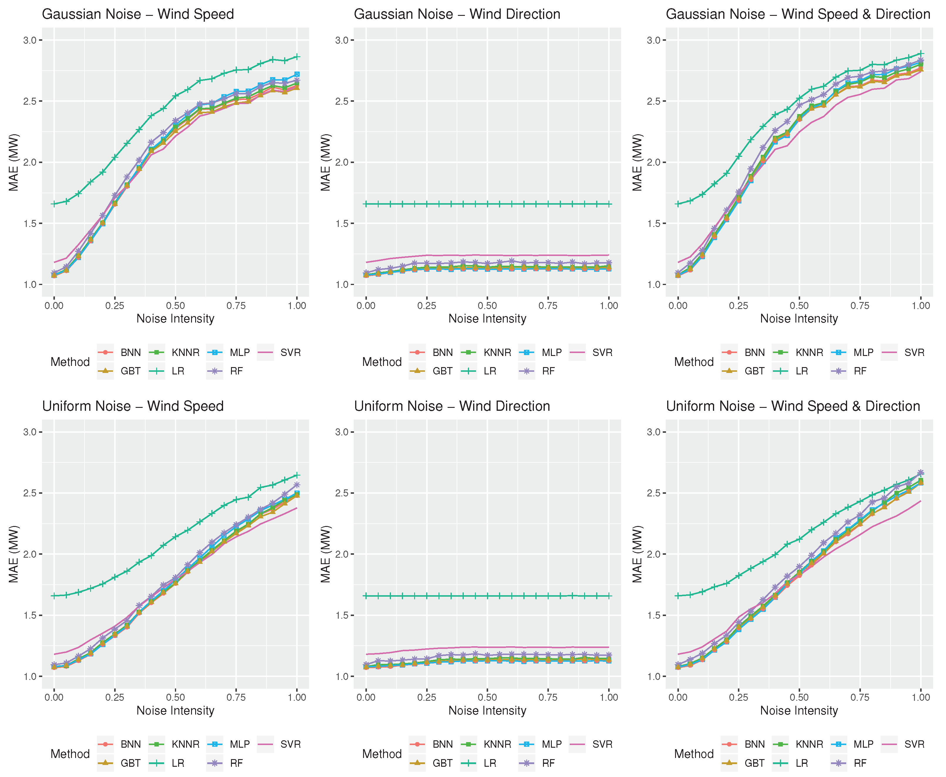
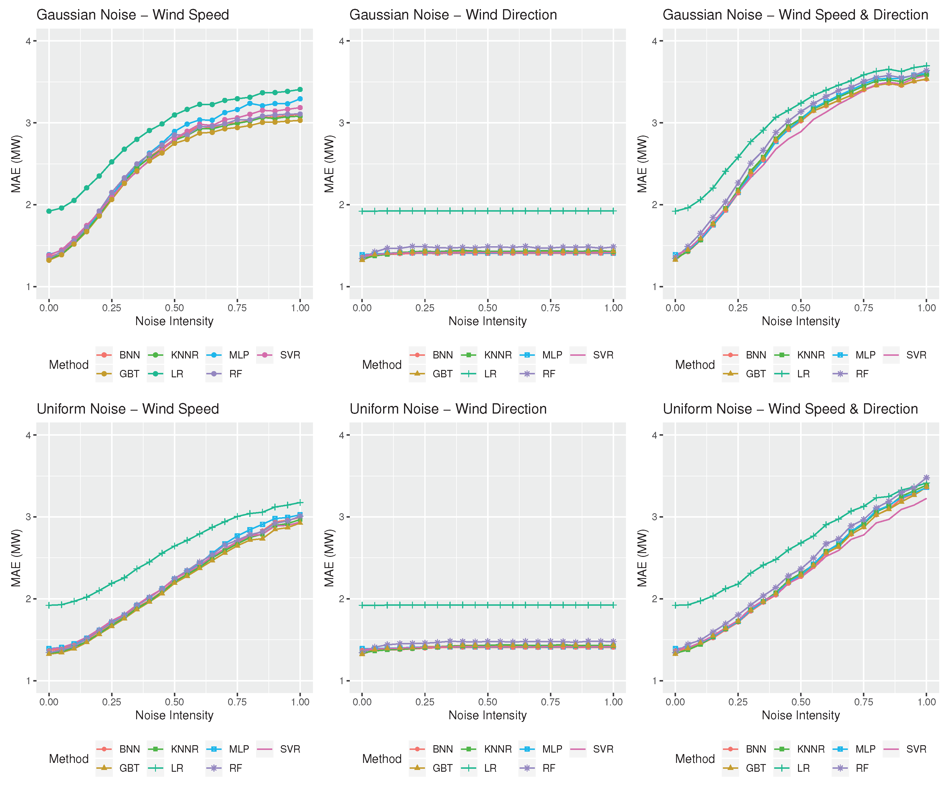
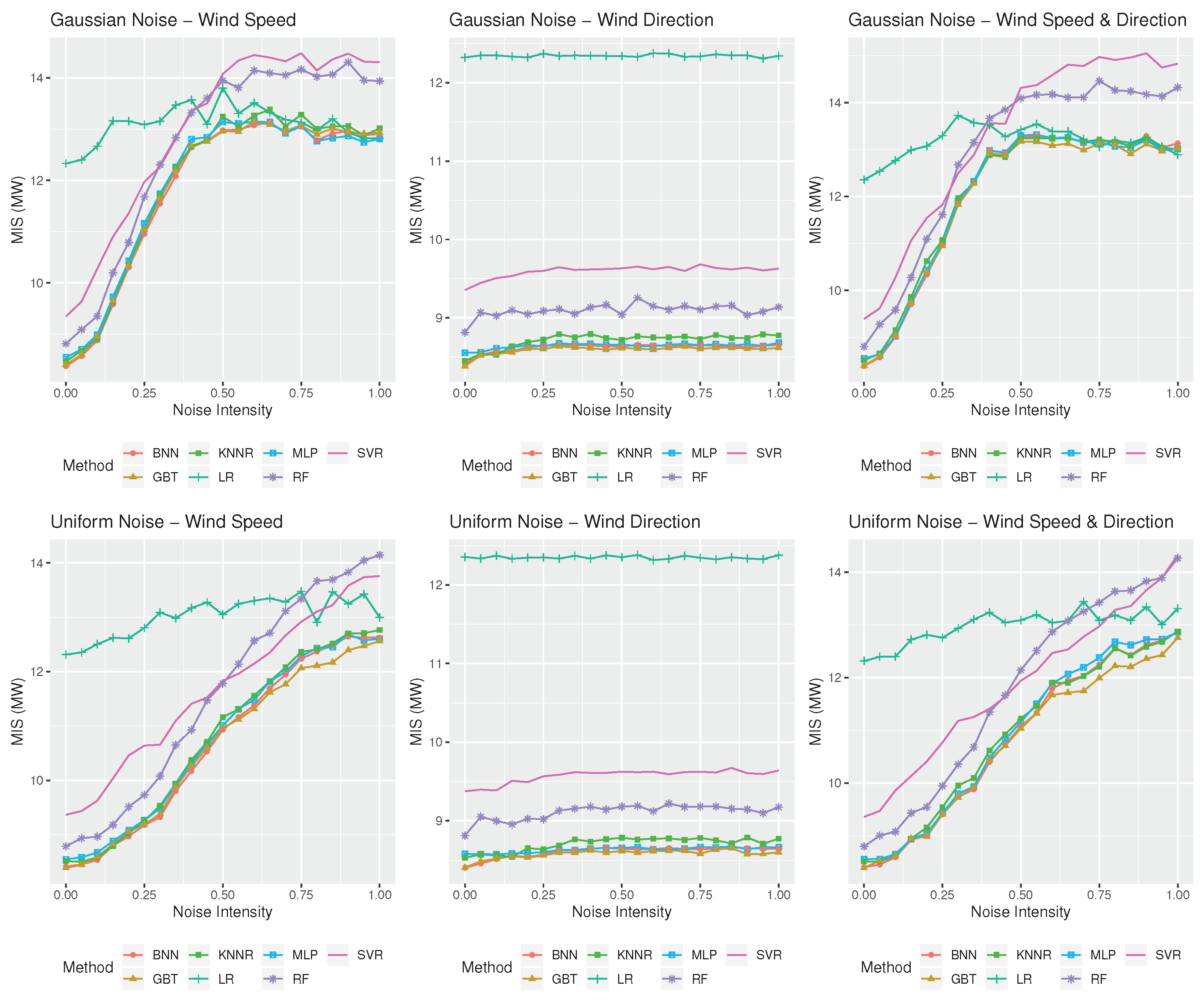
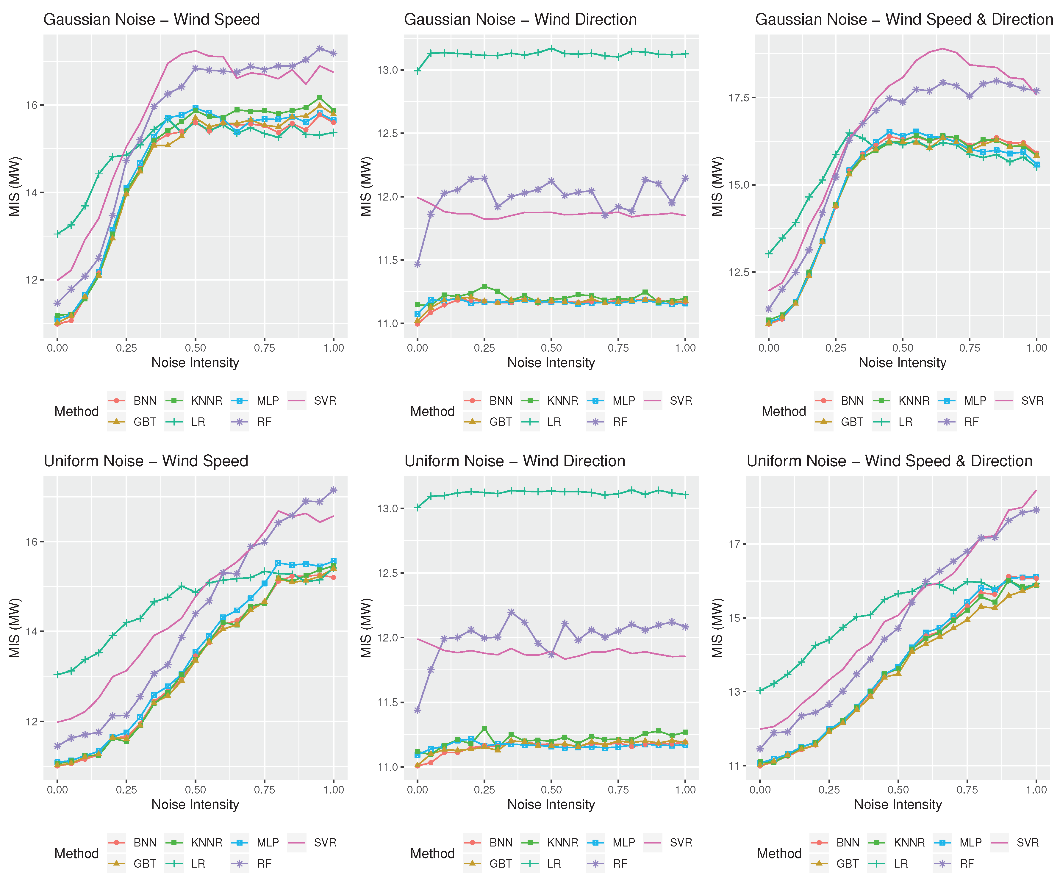
  • Point forecasts and prediction intervals are evaluated using the MAE and MIS measures, respectively;
  • Steps 2 to 9 are repeated for all the five possible combinations of samples;
  • The results are summarized by averaging the forecasting performance of the forecasting methods for all five samples considered.

3.3. Results

Figure 5 and Figure 6 summarize the performance of the forecasting methods considered in this study in terms of point forecast accuracy. From left to right, the three panels on the top display the MAE of the forecasting methods for the case of the Gaussian noise of various intensities σ , applied to wind speed forecasts, wind direction forecasts, and both, respectively. Similarly, the three panels at the bottom display the MAE of the forecasting methods for the case of the uniform noise of various intensities s.
The results look similar for both wind farms, with MAE being gradually increased as wind speed forecasts become more inaccurate, but remaining rather constant as wind direction forecasting accuracy is deteriorated. This indicates that all methods rely heavily on wind speed forecasts for predicting wind power, meaning that imperfect wind direction forecasts have a minor impact to overall accuracy. However, this is not true when imperfect forecasts are provided both for wind speed and direction, as in this scenario, none of the variables provided as predictors are reliable, and therefore, forecasting accuracy is decreased even more.
Another interesting finding is that Gaussian noise seems to have a larger impact on forecasting accuracy than the uniform one. For example, in the Aeolos wind farm, under conditions of both wind speed and direction imperfect forecasts, MAE reaches 2.72 MW and 2.95 MW for uniform and Gaussian noise, respectively. Similarly, in the Rokas wind farm, MAE reaches 3.60 MW and 3.74 MW for uniform and Gaussian noise, respectively. Moreover, the growth rate of MAE differs when different types of noises are considered, with MAE following a linear-like trend for the case of the uniform noise and a sigmoid-like one for the case the Gaussian noise. In this respect, we conclude that imperfect weather forecasts of different particularities may result in different levels of point forecast accuracy.
Regarding the forecasting methods used, in both cases we observe that ML methods outperform LR, especially for small noise intensities. However, these differences become small or even insignificant for highly inaccurate weather forecasts. This highlights the advantage of ML methods in identifying nonlinear dependencies between the target and the predictor variables, which is diminished, however, when weather forecasts are highly inaccurate.
Observe also that different ML methods are more appropriate for predicting wind power under different weather forecast accuracy levels. For example, in the Aeolos wind farm, BNN is the most appropriate forecasting method when a uniform noise of an s value up to 0.50 is considered, both for wind speed and direction, with SVR becoming the most accurate forecasting method for higher noise intensities. Similarly, GBT is the most accurate method for predicting Rokas’ wind power under conditions of perfect foresight, KNNR for s values up to 0.10, BNN for s values up to 0.45, and SVR for s values greater than 0.45. The results are similar for the case of the Gaussian noise. In the Aeolos wind farm, MLP is the most accurate method for a wind speed and direction noise of intensity σ up to 0.30, with SVR being the most accurate method for greater σ values. Accordingly, in the Rokas wind farm, GBT is the best option for predicting wind power under conditions of perfect foresight, followed by BNN for σ values up to 0.45, SVR for σ values up to 0.75, and BNN for even greater σ values.
Drawing from the above, we conclude that not only are ML methods more appropriate for providing wind power forecasts than linear methods, but that different ML methods should be utilized per case based on (i) the type of uncertainty characterizing the weather forecasts and (ii) the extent of that uncertainty. To that end, NNs and GBT, which are highly specialized for solving demanding regression problems, should be preferred when relatively accurate weather forecasts are available, while SVR should be chosen when relatively inaccurate weather forecasts are present.
The results are quite different for the case of the prediction intervals. More specifically, according to Figure 7 and Figure 8, although MIS is gradually increased as wind speed forecasts become more inaccurate, remaining also more or less constant as wind direction forecasting accuracy is deteriorated, the performance of the LR method is comparable to that of the ML ones, especially under conditions of highly inaccurate weather forecasts. In fact, when both wind speed and direction forecasts are highly inaccurate, being also characterized by a Gaussian noise, LR provides the best prediction intervals for the wind farm of Rokas for any σ value greater than 0.5, being also the best performing method for the wind farm of Aeolos for σ values of 0.75 and 1.00. However, ML methods, and especially GBT, perform better in general in both wind farms when a uniform type of noise is considered, regardless of its intensity. Note also that SVR, which was the most robust approach in terms of point forecasts accuracy, is systematically significantly worse than the rest of the methods in providing efficient prediction intervals.
The abovementioned phenomenon can be explained by disaggregating MIS into its two main components: coverage and spread. Given that prediction intervals are empirically derived using a bootstrap approach, the nominal coverage is effectively captured by all the forecasting methods considered equally, even for high noise intensities (coverage ranges from 93% to 97%). However, in order for the methods to achieve such a coverage, the spread of the derived prediction intervals is continuously growing as noise intensity rises. Thus, MIS is increased as uncertainty becomes larger, especially for methods that display extreme errors, although on average they may provide better forecasting accuracy.

4. Discussion

In the previous section, we provided empirical results with regards to the impact of imperfect weather forecasts (wind speed and direction) on forecasting accuracy and uncertainty estimation of wind power generation. The results can be summarized to be dependent on three factors: the type of independent variable, the type of performance indicator considered, and the forecasting methods utilized.
With regards to the independent variables used to predict wind power, we observed that wind speed has a much more significant impact compared to wind direction. Accurately predicting wind speed results in much better forecasts, both in terms of point forecast accuracy as well as prediction intervals estimation. On the other hand, the provision of noisy wind direction forecasts does not significantly affect the forecasting performance of a particular method. When both variables are assumed to be predicted imperfectly, then the forecasting performance drops even further, as it was expected.
The results are heavily dependent on the performance indicator that is used. When focusing on point forecast accuracy (Figure 5 and Figure 6), the performances of the methods show a very stable, negative relationship with the wind speed noise intensity. On the other hand, the performance of the prediction intervals shows a much more volatile behavior. At the same time, Figure 7 and Figure 8 show that the ability of the methods to estimate the wind power generation uncertainty does not always monotonically decrease with the noise intensity; this is particularly true for the statistical model (LR) or when Gaussian noise distributions are assumed.
The third factor relates to the nature of the forecasting methods considered. In our experimentation, we employ both statistical, linear as well as ML, nonlinear approaches. When perfect forecasts of the predictors are available, ML methods provide roughly 25% better predictions compared to the LR statistical benchmark. In this situation, there is little to distinguish with regards to the point forecast accuracy of the ML approaches, apart from the slightly worse performance of SVR compared to other nonlinear approaches. However, the two ML methods, namely RF and SVR, are significantly worse than the others in estimating the uncertainty, resulting in much wider intervals. The superior performance of ML methods over LR becomes less significant as the noise intensity in predicting the wind speed increases. The differences become smaller for higher noise intensities in point forecast accuracy. LR even outperforms several (or all) ML approaches in estimating the uncertainty around wind power generation given highly uncertain wind speed forecasts.
The empirical results presented here could be of particular interest to wind farm operators and managers. Given the location and distance of a weather forecast station, decision makers can decide on the optimal forecasting approach based on the characteristics of the typical weather forecasts that they receive, including noise intensity and distribution. Similar to other forecasting problems, we also notice here a “horses for courses” situation [53] with different approaches being the better options under different conditions. Regardless of the plethora of possible optimal solutions, one common theme seems to be that the statistical approach considered in this paper performs on par (if not better) when the noise intensity is very high [23]. When this is doubled with the fact that LR is multiple times faster than the ML approaches that we examined, the choice of a forecasting model under perfectly imperfect weather forecasts becomes a no-brainer [51,54].
We now return to the research question presented in the introduction section: How does weather forecast uncertainty affect the relative performance of statistical and ML methods for wind power forecasting? The relative performance of statistical versus ML methods for wind power forecasting depends on the (in)accuracy of the wind speed forecast and the performance indicator (point forecast accuracy or performance of the prediction intervals). Increases in the uncertainty of the wind speed improve the performance of statistical methods, relative to machine learning methods. Increases in the uncertainty of the wind direction have a minimal impact on all methods.
While we focus on a very specific context, our results inform the forecasting research with regard to the value of explanatory variables. Our results corroborate the findings of [2]: the added-value of explanatory variables is highly associated with their accuracy. If we are able to forecast them accurately, then the quality of the predictions for the dependent variable increases significantly. If we are unable to accurately forecast wind speed, then it would be probably preferable to utilize time series approaches for forecasting wind power [55].
One limitation of this study relates to our experimental design. Having access to the real weather conditions, we simulated imperfect forecasts under reasonable distributional assumptions. However, it is possible that our results might not generalize if other error distributions for the noise occur. A second limitation has to do with the context of our empirical study. Constrained by data availability, we examined the behavior of two wind farms that are located in similar geographical positions. Our results might differ in other locations or if other contexts (such as photo-voltaic parks) are considered. A third limitation of this study refers to the application of single forecasting models with our recommendations being based on selecting the best method on each occasion. An alternative would be the use of combinations, which has shown good performance in numerous studies [56], even in their simplest forms [57]. Here, we could consider combining the forecasts from all or selected pools of methods [58].

5. Conclusions

In this article, we explored the impact of imperfect weather forecasts on a by and large weather-driven industrial function: wind power generation. In this context, forecasting is essential as to be able to estimate when the wind turbines will work at full capacity, and when at almost no or limited capacity. Wind power needs to be forecast at very high frequencies, and as such, point forecasts and the respective prediction intervals are essential inputs in the broader decision-making process. Two classes of forecasting methods were examined for addressing this task: statistical and ML. In both cases, weather forecasts are an essential input, with their imperfection needing to be assessed in terms of its impact on the final forecasting accuracy.
We performed such an empirical assessment by using a dataset that involves two wind farms and considering various types of imperfect weather forecasts. Our results suggest that ML methods outperform statistical ones in terms of point forecast accuracy, especially for low noise intensities. However, these differences become small for highly inaccurate weather forecasts. This highlights the advantage of ML methods in identifying nonlinear dependencies between the variables taken into consideration, a difference that is vastly diminished when weather forecasts are highly inaccurate. Furthermore, we found out that different ML methods should be utilized per case based on (i) the type of uncertainty characterizing the weather forecasts and (ii) the extent of that uncertainty. To that end, NNs and GBT, which are highly specialized for solving demanding regression problems, should be preferred when relatively accurate weather forecasts are available, while SVR should be chosen when relatively inaccurate weather forecasts are present. The results are quite different for the case of the prediction intervals. Although the precision of the methods is gradually decreased as wind speed forecasts become more inaccurate, the performance of the statistical benchmark is comparable to that of the ML ones, especially under conditions of highly inaccurate weather forecasts. In fact, linear regression provides better forecasts than the ML methods when Gaussian noise distributions of high deviations are assumed.
We do not claim that we have exhaustive results and thus generalization of our findings should be treated with scrutiny. Nevertheless, we do firmly believe that we provide sufficient evidence and motivation in order to drive further studies in this direction. Future research could take many guises, but we do believe that at least the following avenues should, sooner than later, be explored:
  • The “forecasting horserace” should be expanded to include more methods and accuracy measures;
  • Given that the examined dataset includes two predictor variables, i.e., wind speed and direction, bivariate models, inspired by econometric approaches, like VAR models, should be explored;
  • “When in doubt combine”: combinations of all (or the top-three methods) for each forecast case should be tested (for both point forecasts and prediction intervals). Alternatively, one could try to go for a clever selection algorithm in between those ML and statistical methods (see for example [59]), or even hybrid approaches [60];
  • Temporal aggregation is always a way to self-improve any forecasting method (times series or cross-sectional) and this alternative should be employed in any context, especially when it involves a lot of uncertainty or complexity [61]. This could be achieved either via selecting a single aggregation level [62] or via combining the forecasts produced for multiple aggregation levels [63];
  • The provided forecasts should be evaluated “on the money” with real-life (and asymmetric) utility functions.

Author Contributions

Conceptualization, E.S., F.P. and K.N.; methodology, E.S., F.P. and K.N.; software, E.S.; validation, E.S., F.P.; formal analysis, E.S., F.P.; investigation, E.S., F.P. and K.N.; resources, E.S.; data curation, E.S.; writing—original draft preparation, E.S., F.P. and K.N.; writing—review and editing, E.S., F.P. and K.N.; visualization, E.S.; supervision, F.P. and K.N.; project administration, F.P. and K.N. All authors have read and agreed to the published version of the manuscript.

Funding

This research received no external funding.

Acknowledgments

We are grateful to Nikos Hatziargyriou and George Sideratos of the National Technical University of Athens, as well as the EU SafeWind Project for providing the data.

Conflicts of Interest

The authors declare no conflicts of interest.

Abbreviations

The following abbreviations are used in this manuscript:
BNNBayesian Neural Network
GBTGradient Boosting Trees
KNNRK-Nearest Neighbor Regression
LRLinear Regression
MLMachine Learning
NNNeural Network
MLPMulti-Layer Perceptron
RFRandom Forest
RTRegression Tree
SVMSupport Vector Machine
SVRSupport Vector Regression

References

  1. Cai, L.; Gu, J.; Ma, J.; Jin, Z. Probabilistic Wind Power Forecasting Approach via Instance-Based Transfer Learning Embedded Gradient Boosting Decision Trees. Energies 2019, 12, 159. [Google Scholar] [CrossRef] [Green Version]
  2. Bojer, C.; Meldgaard, J. Learnings from Kaggle’s Forecasting Competitions. Work. Paper 2020. [Google Scholar] [CrossRef]
  3. Jeon, J.; Panagiotelis, A.; Petropoulos, F. Probabilistic forecast reconciliation with applications to wind power and electric load. Eur. J. Oper. Res. 2019. [Google Scholar] [CrossRef]
  4. Agüera-Pérez, A.; Palomares-Salas, J.C.; González de la Rosa, J.J.; Florencias-Oliveros, O. Weather forecasts for microgrid energy management: Review, discussion and recommendations. Appl. Energy 2018, 228, 265–278. [Google Scholar] [CrossRef]
  5. Shi, J.; Qu, X.; Zeng, S. Short-Term Wind Power Generation Forecasting: Direct Versus Indirect Arima-Based Approaches. Int. J. Green Energy 2011, 8, 100–112. [Google Scholar] [CrossRef]
  6. Jeon, J.; Taylor, J.W. Using Conditional Kernel Density Estimation for Wind Power Density Forecasting. J. Am. Stat. Assoc. 2012, 107, 66–79. [Google Scholar] [CrossRef] [Green Version]
  7. Cheng, W.Y.Y.; Liu, Y.; Bourgeois, A.J.; Wu, Y.; Haupt, S.E. Short-term wind forecast of a data assimilation/weather forecasting system with wind turbine anemometer measurement assimilation. Renew. Energy 2017, 107, 340–351. [Google Scholar] [CrossRef]
  8. Zhang, W.; Maleki, A.; Rosen, M.A.; Liu, J. Sizing a stand-alone solar-wind-hydrogen energy system using weather forecasting and a hybrid search optimization algorithm. Energy Convers. Manag. 2019, 180, 609–621. [Google Scholar] [CrossRef]
  9. Dupré, A.; Drobinski, P.; Alonzo, B.; Badosa, J.; Briard, C.; Plougonven, R. Sub-hourly forecasting of wind speed and wind energy. Renew. Energy 2020, 145, 2373–2379. [Google Scholar] [CrossRef]
  10. Hong, T.; Wang, P.; White, L. Weather station selection for electric load forecasting. Int. J. Forecast. 2015, 31, 286–295. [Google Scholar] [CrossRef]
  11. Lai, S.H.; Hong, T. When One Size No Longer Fits All: Electric Load Forecasting with a Geographic Hierarchy; SAS White Paper; SAS: Cary, NC, USA, 2013. [Google Scholar]
  12. Barbounis, T.G.; Theocharis, J.B.; Alexiadis, M.C.; Dokopoulos, P.S. Long-term wind speed and power forecasting using local recurrent neural network models. IEEE Trans. Energy Convers. 2006, 21, 273–284. [Google Scholar] [CrossRef]
  13. Sun, W.; Liu, M. Wind speed forecasting using FEEMD echo state networks with RELM in Hebei, China. Energy Convers. Manag. 2016, 114, 197–208. [Google Scholar] [CrossRef]
  14. Al-Zadjali, S.; Al Maashri, A.; Al-Hinai, A.; Al-Yahyai, S.; Bakhtvar, M. An Accurate, Light-Weight Wind Speed Predictor for Renewable Energy Management Systems. Energies 2019, 12, 4355. [Google Scholar] [CrossRef] [Green Version]
  15. Ren, Y.; Li, H.; Lin, H.C. Optimization of Feedforward Neural Networks Using an Improved Flower Pollination Algorithm for Short-Term Wind Speed Prediction. Energies 2019, 12, 4126. [Google Scholar] [CrossRef] [Green Version]
  16. Cassola, F.; Burlando, M. Wind speed and wind energy forecast through Kalman filtering of Numerical Weather Prediction model output. Appl. Energy 2012, 99, 154–166. [Google Scholar] [CrossRef]
  17. Ding, M.; Zhou, H.; Xie, H.; Wu, M.; Nakanishi, Y.; Yokoyama, R. A gated recurrent unit neural networks based wind speed error correction model for short-term wind power forecasting. Neurocomputing 2019, 365, 54–61. [Google Scholar] [CrossRef]
  18. Sun, S.; Fu, J.; Li, A. A Compound Wind Power Forecasting Strategy Based on Clustering, Two-Stage Decomposition, Parameter Optimization, and Optimal Combination of Multiple Machine Learning Approaches. Energies 2019, 12, 3586. [Google Scholar] [CrossRef] [Green Version]
  19. Demolli, H.; Dokuz, A.S.; Ecemis, A.; Gokcek, M. Wind power forecasting based on daily wind speed data using machine learning algorithms. Energy Convers. Manag. 2019, 198, 111823. [Google Scholar] [CrossRef]
  20. Liu, H.; Shi, J.; Erdem, E. An Integrated Wind Power Forecasting Methodology: Interval Estimation of Wind Speed, Operation Probability Of Wind Turbine, And Conditional Expected Wind Power Output of A Wind Farm. Int. J. Green Energy 2013, 10, 151–176. [Google Scholar] [CrossRef]
  21. Liu, H.; Shi, J.; Qu, X. Empirical investigation on using wind speed volatility to estimate the operation probability and power output of wind turbines. Energy Convers. Manag. 2013, 67, 8–17. [Google Scholar] [CrossRef]
  22. Salfate, I.; López-Caraballo, C.H.; Sabín-Sanjulián, C.; Lazzús, J.A.; Vega, P.; Cuturrufo, F.; Marín, J. 24-hours wind speed forecasting and wind power generation in La Serena (Chile). Wind Eng. 2018, 42, 607–623. [Google Scholar] [CrossRef]
  23. Makridakis, S.; Spiliotis, E.; Assimakopoulos, V. Statistical and Machine Learning forecasting methods: Concerns and ways forward. PLoS ONE 2018, 13, e0194889. [Google Scholar] [CrossRef] [PubMed] [Green Version]
  24. Spiliotis, E.; Nikolopoulos, K.; Assimakopoulos, V. Tales from tails: On the empirical distributions of forecasting errors and their implication to risk. Int. J. Forecast. 2019, 35, 687–698. [Google Scholar] [CrossRef]
  25. Kohavi, R. A Study of Cross-Validation and Bootstrap for Accuracy Estimation and Model Selection. In The 14th International Joint Conference on Artificial Intelligence; Morgan Kaufmann: San Francisco, CA, USA, 1995; Volume 2, pp. 1137–1143. [Google Scholar]
  26. Zhang, G.; Patuwo, B.E.; Hu, M.Y. Forecasting with artificial neural networks: The state of the art. Int. J. Forecast. 1998, 14, 35–62. [Google Scholar] [CrossRef]
  27. Lippmann, R.P. An Introduction to Computing with Neural Nets. IEEE ASSP Mag. 1987, 4, 4–22. [Google Scholar] [CrossRef]
  28. Møller, M.F. A scaled conjugate gradient algorithm for fast supervised learning. Neural Netw. 1993, 6, 525–533. [Google Scholar] [CrossRef]
  29. Kourentzes, N.; Barrow, D.K.; Crone, S.F. Neural network ensemble operators for time series forecasting. Expert Syst. Appl. 2014, 41, 4235–4244. [Google Scholar] [CrossRef] [Green Version]
  30. Bergmeir, C.; Benítez, J.M. Neural Networks in R Using the Stuttgart Neural Network Simulator: RSNNS. J. Stat. Softw. 2012, 46, 1–26. [Google Scholar] [CrossRef] [Green Version]
  31. MacKay, D.J.C. Bayesian Interpolation. Neural Comput. 1992, 4, 415–447. [Google Scholar] [CrossRef]
  32. Dan Foresee, F.; Hagan, M.T. Gauss-Newton approximation to bayesian learning. In Proceedings of the IEEE International Conference on Neural Networks, Houston, TX, USA, 12 June 1997; Volume 3, pp. 1930–1935. [Google Scholar] [CrossRef]
  33. Nguyen, D.; Widrow, B. Improving the learning speed of 2-layer neural networks by choosing initial values of the adaptive weights. IJCNN Int. Jt. Conf. Neural Netw. 1990, 13, 21–26. [Google Scholar] [CrossRef]
  34. Rodriguez, P.P.; Gianola, D. brnn: Bayesian Regularization for Feed-Forward Neural Networks. 2018. R Package Version 0.7. Available online: https://CRAN.R-project.org/package=brnn (accessed on 15 February 2020).
  35. Breiman, L. Classification and Regression Trees; Chapman & Hall: Boca Raton, FL, USA, 1993. [Google Scholar]
  36. Breiman, L. Random Forests. Mach. Learn. 2001, 45, 5–32. [Google Scholar] [CrossRef] [Green Version]
  37. Liaw, A.; Wiener, M. Classification and Regression by randomForest. R News 2002, 2, 18–22. [Google Scholar]
  38. Freund, Y.; Schapire, R.E. A Decision-Theoretic Generalization of On-Line Learning and an Application to Boosting. J. Comput. Syst. Sci. 1997, 55, 119–139. [Google Scholar] [CrossRef] [Green Version]
  39. Friedman, J.H. Stochastic gradient boosting. Comput. Stat. Data Anal. 2002, 38, 367–378. [Google Scholar] [CrossRef]
  40. Greenwell, B.; Boehmke, B.; Cunningham, J.; Developers, G. gbm: Generalized Boosted Regression Models. 2019. R Package Version 2.1.5. Available online: https://CRAN.R-project.org/package=gbm (accessed on 15 February 2020).
  41. Kuhn, M. Caret: Classification and Regression Training. 2018. R Package Version 6.0-81. Available online: https://CRAN.R-project.org/package=caret (accessed on 15 February 2020).
  42. Schölkopf, B.; Smola, A.J. Learning with kernel: Support Vector Machines, Regularization, Optimization and Beyond; The MIT Press: Cambridge, MA, USA, 2001. [Google Scholar]
  43. Meyer, D.; Dimitriadou, E.; Hornik, K.; Weingessel, A.; Leisch, F. e1071: Misc Functions of the Department of Statistics, Probability Theory Group (Formerly: E1071), TU Wien. 2019. R Package Version 1.7-1. Available online: https://CRAN.R-project.org/package=e1071 (accessed on 15 February 2020).
  44. Vahidzadeh, M.; Markfort, C.D. An Induction Curve Model for Prediction of Power Output of Wind Turbines in Complex Conditions. Energies 2020, 13, 891. [Google Scholar] [CrossRef] [Green Version]
  45. Luo, J.; Hong, T.; Fang, S.C. Benchmarking robustness of load forecasting models under data integrity attacks. Int. J. Forecast. 2018, 34, 89–104. [Google Scholar] [CrossRef]
  46. Khosravi, A.; Nahavandi, S.; Creighton, D.; Atiya, A.F. Comprehensive Review of Neural Network-Based Prediction Intervals and New Advances. IEEE Trans. Neural Netw. 2011, 22, 1341–1356. [Google Scholar] [CrossRef]
  47. Spiliotis, E.; Assimakopoulos, V.; Makridakis, S. Generalizing the Theta method for automatic forecasting. Eur. J. Oper. Res. 2020. [Google Scholar] [CrossRef]
  48. Efron, B. Bootstrap methods: Another look at the jackknife. Ann. Stat. 1979, 7, 1–26. [Google Scholar] [CrossRef]
  49. Heskes, T. Practical confidence and prediction intervals. Neural Inf. Process. Syst. 1997, 9, 176–182. [Google Scholar]
  50. Gneiting, T.; Raftery, A. Strictly proper scoring rules, prediction, and estimation. J. Am. Stat. Assoc. 2007, 102, 359–378. [Google Scholar] [CrossRef]
  51. Makridakis, S.; Spiliotis, E.; Assimakopoulos, V. The M4 Competition: 100,000 time series and 61 forecasting methods. Int. J. Forecast. 2020, 36, 54–74. [Google Scholar] [CrossRef]
  52. Yu, X.; Zhang, W.; Zang, H.; Yang, H. Wind Power Interval Forecasting Based on Confidence Interval Optimization. Energies 2018, 11, 3336. [Google Scholar] [CrossRef] [Green Version]
  53. Petropoulos, F.; Makridakis, S.; Assimakopoulos, V.; Nikolopoulos, K. ‘Horses for Courses’ in demand forecasting. Eur. J. Oper. Res. 2014, 237, 152–163. [Google Scholar] [CrossRef] [Green Version]
  54. Nikolopoulos, K.; Petropoulos, F. Forecasting for big data: Does suboptimality matter? Comput. Oper. Res. 2018, 98, 322–329. [Google Scholar] [CrossRef] [Green Version]
  55. Makridakis, S.; Hyndman, R.J.; Petropoulos, F. Forecasting in social settings: The state of the art. Int. J. Forecast. 2020, 36, 15–28. [Google Scholar] [CrossRef]
  56. Kim, Y.; Hur, J. An Ensemble Forecasting Model of Wind Power Outputs based on Improved Statistical Approaches. Energies 2020, 13, 1071. [Google Scholar] [CrossRef] [Green Version]
  57. Petropoulos, F.; Svetunkov, I. A simple combination of univariate models. Int. J. Forecast. 2020, 36, 110–115. [Google Scholar] [CrossRef]
  58. Kourentzes, N.; Barrow, D.; Petropoulos, F. Another look at forecast selection and combination: Evidence from forecast pooling. Int. J. Prod. Econ. 2019, 209, 226–235. [Google Scholar] [CrossRef] [Green Version]
  59. Nikolopoulos, K. Forecasting with quantitative methods: The impact of special events in time series. Appl. Econ. 2010, 42, 947–955. [Google Scholar] [CrossRef]
  60. Shi, J.; Guo, J.; Zheng, S. Evaluation of hybrid forecasting approaches for wind speed and power generation time series. Renew. Sustain. Energy Rev. 2012, 16, 3471–3480. [Google Scholar] [CrossRef]
  61. Spiliotis, E.; Petropoulos, F.; Kourentzes, N.; Assimakopoulos, V. Cross-temporal aggregation: Improving the forecast accuracy of hierarchical electricity consumption. Appl. Energy 2020, 261, 114339. [Google Scholar] [CrossRef]
  62. Nikolopoulos, K.; Syntetos, A.A.; Boylan, J.E.; Petropoulos, F.; Assimakopoulos, V. An aggregate–disaggregate intermittent demand approach (ADIDA) to forecasting: An empirical proposition and analysis. J. Oper. Res. Soc. 2011, 62, 544–554. [Google Scholar] [CrossRef] [Green Version]
  63. Kourentzes, N.; Petropoulos, F.; Trapero, J.R. Improving forecasting by estimating time series structural components across multiple frequencies. Int. J. Forecast. 2014, 30, 291–302. [Google Scholar] [CrossRef] [Green Version]
Figure 1. Wind power (measured in MV) compared with wind direction (degrees) and speed (m/s) for the Aeolos farm. The panels represent the empirical power curves of the farm, being subject to wind direction (left) and speed (right), respectively.
Energies 13 01880 g001
Figure 2. Wind power (MV) compared with wind direction (degrees) and speed (m/s) for the Rokas farm. The panels represent the empirical power curves of the farm, being subject to wind direction (left) and speed (right), respectively.
Energies 13 01880 g002
Figure 3. Wind roses providing a view of how wind speed and direction are distributed at the Aeolos (left) and Rokas (right) wind farms.
Energies 13 01880 g003
Figure 4. Weibull distributions of the wind speed at the Aeolos (left) and Rokas (right) wind farms.
Energies 13 01880 g004
Figure 5. Forecasting performance in terms of wind power point forecasts (mean absolute error (MAE), measured in MW) of the statistical and machine learning (ML) methods considered in this study for the Aeolos wind farm when different types of noise and noise intensities are considered. The three panels on the top display the accuracy of the methods for the case of the Gaussian noise of various intensities, σ , applied to wind speed forecasts, wind direction forecast, and both, respectively. The three panels at the bottom display the same results for the case of the uniform noise of various intensities s.
Energies 13 01880 g005
Figure 6. Forecasting performance in terms of wind power point forecasts (MAE, measured in MW) of the statistical and ML methods considered in this study for the Rokas wind farm when different types of noise and noise intensities are considered. The three panels on the top display the accuracy of the methods for the case of the Gaussian noise of various intensities, σ , applied to wind speed forecasts, wind direction forecast, and both, respectively. The three panels at the bottom display the same results for the case of the uniform noise of various intensities s.
Energies 13 01880 g006
Figure 7. Forecasting performance in terms of wind power prediction intervals (Mean Interval Score (MIS), measured in MW) of the statistical and ML methods considered in this study for the Aeolos wind farm when different types of noise and noise intensities are considered. The three panels on the top display the accuracy of the methods for the case of the Gaussian noise of various intensities, σ , applied to wind speed forecasts, wind direction forecast, and both, respectively. The three panels at the bottom display the same results for the case of the uniform noise of various intensities s.
Energies 13 01880 g007
Figure 8. Forecasting performance in terms of wind power prediction intervals (MIS, measured in MW) of the statistical and ML methods considered in this study for the Rokas wind farm when different types of noise and noise intensities are considered. The three panels on the top display the accuracy of the methods for the case of the Gaussian noise of various intensities, σ , applied to wind speed forecasts, wind direction forecast, and both, respectively. The three panels at the bottom display the same results for the case of the uniform noise of various intensities s.
Energies 13 01880 g008

