Daily Crude Oil Price Forecasting Based on Improved CEEMDAN, SCA, and RVFL: A Case Study in WTI Oil Market

Abstract

Crude oil is one of the strategic energies and plays an increasingly critical role effecting on the world economic development. The fluctuations of crude oil prices are caused by various extrinsic and intrinsic factors and usually demonstrate complex characteristics. Therefore, it is a great challenge for accurately forecasting crude oil prices. In this study, a self-optimizing ensemble learning model incorporating the improved complete ensemble empirical mode decomposition with adaptive noise (ICEEMDAN), sine cosine algorithm (SCA), and random vector functional link (RVFL) neural network, namely ICEEMDAN-SCA-RVFL, is proposed to forecast crude oil prices. Firstly, we employ ICEEMDAN to decompose the raw series of crude oil prices into a group of relatively simple subseries. Secondly, RVFL is used to forecast the target values for each decomposed subseries individually. Due to the complex parameter settings of ICEEMDAN and RVFL, SCA is introduced to optimize the parameters for ICEEMDAN and RVFL in the above decomposition and prediction stages simultaneously. Finally, we assemble the predicted values of all individual subseries as the final predicted values of crude oil prices. Our proposed ICEEMDAN-SCA-RVFL significantly outperforms the single and ensemble benchmark models, as demonstrated by a case study conducted using the time series of West Texas Intermediate (WTI) daily crude oil spot prices.

1. Introduction

As one type of the main energy sources, crude oil has a great impact on the world’s economic development. Given the importance of crude oil, the fluctuations of its prices have attracted worldwide attention. Since a variety of extrinsic and intrinsic factors are able to influence crude oil prices, crude oil price series usually demonstrates nonlinearity and nonstationarity, making it difficult to accurately forecast [1,2,3]. Therefore, crude oil price forecasting has always been a research hotspot. In previous research, various prediction approaches were developed to forecast crude oil prices. In general, these prediction approaches fall into two categories: (1) statistical approaches, and (2) artificial intelligence (AI) approaches. The main statistical approaches for crude oil price forecasting include error correction model (ECM) [4], hidden Markov model (HMM) [5], autoregressive integrated moving average (ARIMA) [6] model, generalized autoregressive conditional heteroskedasticity (GARCH) [7] model, etc. Lanza et al. used cointegration and ECM to analyse the dynamics of crude oil prices [4]. Silva et al. used HMM to estimate the probability distribution of the crude oil price return in short term [5]. Xiang et al. employed ARIMA model to analyse and predict Brent crude oil prices from November 2012 to April 2013, and the experimental result demonstrated that ARIMA could achieve satisfactory short-term prediction results [6]. Wei et al. developed a series of linear and nonlinear GARCH models to analyse the fluctuation of international crude oil markets, and the experimental results exhibited satisfactory forecasting accuracy [7].

Common statistical approaches are able to be applied to linear or near-linear time series forecasting and achieve satisfactory prediction performance. Unfortunately, the raw series of crude oil prices usually involves the complex characteristics and demonstrates nonlinearity and nonstationarity, making it difficult to obtain good prediction performance using traditional statistical approaches [8,9,10]. In recent years, more and more AI approaches were proposed for crude oil price forecasting. The main AI prediction approaches include artificial neural networks (ANN) [11,12], support vector machine (SVM) [13,14], sparse Bayesian learning (SBL) [15], extreme learning machine (ELM) [16], extreme gradient boosting (XGBoost) [17], random vector functional link neural network (RVFL) [18], recurrent neural network(RNN) [19], etc. Mostafa et al. employed an ANN model to predict the crude oil price data between 2 January 1986 and 12 June 2012 [11]. Xie et al. forecasted crude oil prices using a novel SVM-based method, and the experimental results showed that SVM was superior to ARIMA and ANN for crude oil price prediction [13]. Wang et al. constructed ELM models with variant forecasting scheme for short-run crude oil price forecasting [16]. Gumus et al. used XGBoost to interpret the parameters which were the factors affecting crude oil prices [17]. Tang et al. employed a RVFL model using direct input-output links and fixed weights to forecast crude oil prices [18]. Tang et al. developed a multiple wavelet RNN (MWRNN) prediction model for crude oil price forecasting and the prediction model achieved high prediction accuracy [19].

To further enhance prediction performance, many hybrid prediction models were developed for crude oil price forecasting. Yu et al. proposed a hybrid prediction approach incorporating least squares support vector regression (LSSVR) with genetic algorithm (GA) for crude oil price forecasting [20]. Chen et al. proposed a hybrid grey wave prediction model combined RWM/autoregressive moving average (ARMA) to forecast crude oil prices [21]. Wang et al. integrated a rule-based expert system (RES) and ANN to improve the prediction performance of crude oil prices [22]. Tehrani introduced feed forward neural networks (FNN) with GA optimization to construct a hybrid prediction model for crude oil spot price forecasting [23]. In general, these hybrid prediction models are able to integrate the advantages of each single approach, and thus achieve better prediction performance.

Due to the complex characteristics of some raw time series, it is difficult to achieve satisfactory prediction performance only using these raw time series. To cope with that, a “decomposition and ensemble” framework was widely introduced into time series forecasting. The first step of the “decomposition and ensemble” framework is to decompose the complex raw time series into a group of relatively simple components, then a single predictor is introduced to predict each component independently, and finally these predicted values of all components are assembled as the final predicted results [24,25,26,27]. This idea has also been introduced into the field of crude oil price prediction. The complex raw series of crude oil prices is decomposed into several subseries, and then a single predictor is used to predict each subseries, followed by the ensemble of individual predicted results as the final prediction results. In these ensemble models, the decomposition of raw time series is the first step. The main decomposition approaches include wavelet decomposition (WD), independent component analysis (ICA), and empirical mode decomposition (EMD) class methods, etc. Bao et al. integrated WD and least squares support machines (LSSVM) to build an ensemble prediction model to forecast oil prices [28]. He et al. used the heterogeneous features of crude oil price movement to build a novel multivariate EMD-based model in international crude oil markets [29]. Li et al. developed a new ensemble model that incorporated ICEEMDAN with ridge regression (RR) for crude oil price prediction [24].

In the stage of prediction, several optimization algorithms were combined with predictors and been used to further improve the prediction performance. Li et al. proposed a relevance vector machine (RVM) with combined kernel based on particle swarm optimization (PSO) to forecast crude oil prices [30]. Liu et al. developed a regularized extreme learning machine (RELM) network optimized by grey wolf optimizer (GWO) for wind speed forecasting [31].

The above literature has demonstrated the effectiveness of “decomposition and ensemble” framework for the prediction of crude oil prices. In this framework, the selection of decomposition approach and predictor is essential for the improvement of forecasting performance. In view of the potential of ICEEMDAN, sine cosine algorithm (SCA), and RVFL in the decomposition, optimization, and prediction fields respectively, we developed a novel ensemble prediction model incorporating ICEEMDAN, SCA and RVFL, namely ICEEMDAN-SCA-RVFL, for crude oil price forecasting. Firstly, ICEEMDAN is used to decompose the complex raw time series of crude oil prices into a group of relatively simple subseries. Secondly, we apply RVFL to predict the target values of each decomposed subseries individually. Because of the complex parameter settings of ICEEMDAN and RVFL, SCA is introduced to search the optimum parameters for ICEEMDAN and RVFL simultaneously. Finally, the predicted results of all individual subseries are assembled as the final predicted crude oil prices.

The contributions of this study are as follows.

(1)

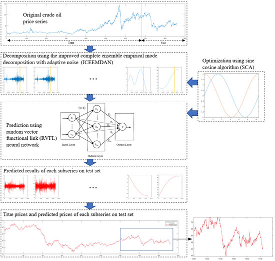
We develop a self-optimizing ensemble learning paradigm incorporating ICEEMDAN, SCA, and RVFL for crude oil price forecasting. To our knowledge, this is the first time that the ensemble framework is introduced into the field of crude oil price forecasting.

(2)

To further enhance forecasting performance, SCA is employed to optimize the parameter settings for ICEEMDAN and RVFL.

(3)

The experiments show that our proposed ICEEMDAN-SCA-RVFL is significantly superior to the single and ensemble benchmark models for crude oil price forecasting.

The main novelty of this study involves the following three aspects: (1) Inspired by the effective decomposition of ICEEMDAN, the powerful optimization ability of SCA and the potential prediction performance of RVFL, a novel ensemble model incorporating the three methods is developed for crude oil price forecasting; (2) SCA is first applied to optimizing the decomposition method ICEEMDAN and prediction method RVFL simultaneously; (3) The proposed ICEEMDAN-SCA-RVFL ensemble model is first developed for the prediction of crude oil prices and the experimental results verify the effectiveness of the prediction model.

The remainder of the paper is organised as follows. First, Section 2 provides a short introduction to ICEEMDAN, SCA, and RVFL. Section 3 explains in elaborate detail the proposed ICEEMDAN-SCA-RVFL. Section 4 reports and discusses the experimental results on WTI daily crude oil price forecasting, followed by the conclusions in Section 5.

2. Preliminaries

2.1. Improved Complete Ensemble Empirical Mode Decomposition with Adaptive Noise (ICEEMDAN)

EMD is first proposed for the decomposition of time series in EMD class methods but suffers from the so-called mode mixing problem [32]. To address this issue, Ensemble EMD (EEMD) was proposed by averaging the results of performing the EMD many times on the raw time series with added Gaussian white noise [33]. However, EEMD introduces a new problem to signal decomposition, i.e., the recovered signal from the components by EEMD may include residual noise. To further improve the performance of EEMD, Torres et al. first proposed a new decomposition approach called complete EEMD with adaptive noise (CEEMDAN) [34]. In this method, an adaptive white noise is added at each stage of the decomposition and it can improve the quality of reconstructing the original signals and provide a better spectral separation of intrinsic mode functions (IMFs). Compared with EEMD, the CEEMDAN reduces the number of sifting iterations and the reconstruction error, resulting in the reduction of computational cost. Later, the authors also proposed an improved CEEMDAN (ICEEMDAN) that is able to handle the problem of residual noise very well [35]. Due to its effectiveness, the ICEEMDAN method is widely used in energy forecasting [36,37,38]. Therefore, we consider using it to decompose raw crude oil price series in this study.

2.2. Sine Cosine Algorithm (SCA)

As one of the novel intelligent optimization algorithms, sine cosine algorithm (SCA) was proved to be superior to PSO, GA, and differential evolution (DE) in convergence accuracy and speed [39,40,41]. SCA first randomly generates the positions of N individuals. Suppose the position of an individual in SCA represents a possible solution to an optimization problem, and use $X_i={(X_{i,1},X_{i,2},\cdots ,X_{i,D})}^T$ to represent the location of the i-th individual, where D denotes the dimension of optimization problem. The best location for all individuals to pass through is represented by $P_b={(P_{b,1},P_{b,2},\cdots ,P_{b,D})}^T$. With evolution, the position of the i-th individual will be updated as:

$$X_{i,d}^{t+1}=\left\{\begin{array}{cc}{X}_{i,d}^t+r_1\times sin\left(r_2\right)\times \left|r_3{P}_{b,d}^t-X_{i,d}^t\right|,\hfill & r_4<0.5\hfill \\ X_{i,d}^t+r_1\times cos\left(r_2\right)\times \left|r_3{P}_{b,d}^t-X_{i,d}^t\right|,\hfill & r_4\ge 0.5\hfill \end{array},\right.$$

(1)

where $X_{i,d}^t$ is the location of the $d-$th dimension $(d=1,2,\cdots ,D)$ of the $i-$th individual current solution at the t-th iteration, $P_{b,d}$ is the position of the destination point in the d-th dimension, $r_1$ is a variable number, and $r_2/r_3/r_4$ are random numbers in specified ranges.

The parameter $r_1$ has an important impact on balancing the abilities of global exploration and local exploitation for SCA. It defines the magnitude of the range of sine and cosine functions, and it also determines the solution move towards or outwards the destinations. Typically, $r_1$ linearly decreases as follows:

$$r_1=a-t\frac{a}{T},$$

(2)

where a is a constant, and t and T denote the current and the maximum number of iteration, respectively.

The parameter $r_2$ is a random number in $[0,2\pi ]$ that defines the moving distance of the next iteration, while $r_3$ and $r_4$ are random numbers that fall in the range of $[0,2]$ and $[0,1]$, respectively. Based on the change of sine and cosine function values to achieve the optimal search, SCA is simple and is easy to implement. Due to its efficient optimization ability, the SCA algorithm was widely used in different optimization problems [42,43].

2.3. Random Vector Functional Link (RVFL) Neural Network

Random vector functional link (RVFL) neural network, whose architecture is illustrated in Figure 1, is a typical feedforward single hidden layer neural network presented in 1992 [44]. Similar to the traditional neural network, the RVFL network consists of three types of layers: input layer, hidden layer and output layer. The difference regarding the structure lies in that RVFL can connect the nodes in the input layer and those in the output layer directly. The RVFL network is a type of non-iterative network that randomly fixes the input weights as well as the biases and then optimizes other parameters via a pseudoinverse [18,44].

With this architecture, the inputs of each node in the output layer come from two parts: input nodes (nodes in the input layer) and enhancement nodes (nodes in the hidden layer). The first part from the input nodes can be treated as a linear combination representing by ${\sum }_{i=1}^n{\theta }_i{x}_i$, while the second part from the enhancement nodes can be denoted by ${\sum }_{i=1}^m{\beta }_{i}g(w_i^{T}X+b_i)$, where n and m are the numbers of input nodes and enhancement nodes respectively, ${\theta }_i$ is the weight of the i-th input node, $w_i$ and $b_i$ are the weight and bias of the i-th enhancement node, $X=[x_1,x_2,\cdots ,x_n]$ is the input, and $g(·)$ is the activation function. Therefore, the total input of the output node can be represented as:

$$y=f\left(X\right)=\sum _{i=1}^n{\theta }_i{x}_i+\sum _{i=1}^m{\beta }_{i}g(w_i^{T}X+b_i).$$

(3)

RVFL fixes $w_i$ and $b_i$ using random numbers of a specified distribution, and then simultaneously optimizes the weights of ${\theta }_i$ and ${\beta }_i$ by minimizing the following system error [18]:

$$E=\frac{1}{2N}\sum _{j=1}^N{(t^{\left(j\right)}-W{d}^{\left(j\right)})}^2,$$

(4)

where N is the number of training samples whose target vector is t, W is the combination of weight ${\theta }_i(i=1,2,\cdots ,n)$ and ${\beta }_i(i=1,2,\cdots ,m)$, and d is a vector combined by the enhancement nodes and input nodes [18,44].

RVFL has a better training speed and can be updated quickly, and it also has fine nonlinear fitting ability [45]. Hence it has been widely used in various fields including energy related forecasting [18,46].

3. ICEEMDAN-SCA-RVFL: The Proposed Approach for Crude Oil Price Forecasting

Following the idea of “decomposition and ensemble”, we develop a self-optimizing ensemble model that combines ICEEMDAN, SCA, and RVFL, termed as ICEEMDAN-SCA-RVFL, to predict crude oil spot prices. Our proposed ensemble model involves three stages as demonstrated in Figure 2.

Stage 1: Decomposition. ICEEMDAN with SCA optimization is proposed to decompose the raw series of crude oil prices into: (1) N IMFs: $IM{F}_i(i=1,2,\cdots ,N)$; (2) one residue R.

Stage 2: Individual forecasting. The each IMF or residue is equally split into a training data set and a test data set. The each RVFL prediction model based on SCA optimization is independently trained on each training data set, and then the prediction model is applied to each test data set accordingly.

Stage 3: Ensemble. The predicted values of all decomposed components are assembled as the final predicted results using addition aggregation.

Our proposed ICEEMDAN-SCA-RVFL uses the framework of “divide and conquer” that was widely used in image processing, fault diagnosis, and so on [47,48,49,50,51]. Firstly, ICEEMDAN is used to divide the nonlinear and nonstationary series of crude oil prices into a group of relatively simple subseries, including several IMFs and one residue. Secondly, RVFL using SCA optimization is applied to each decomposed subseries to build the prediction models. we choose RVFL as the predictor because it was proven effective for time series forecasting in previous research [18,52,53]. Since ICEEMDAN and RVFL have many parameters, it is hard to set the optimum for them in advance. To solve this problem, SCA is introduced to search the optimum parameters for RVFL as well as ICEEMDAN, which can effectively improve the prediction performance of each individual subseries. Finally, the predicted values by RVFL models for each decomposed subseries are assembled as the final predicted crude oil prices using addition aggregation. The “decomposition and ensemble” of ICEEMDAN-SCA-RVFL would contribute to the performance improvement of crude oil price forecasting.

It’s worth mentioning that some recent research also apply RVFL model to forecast crude oil price series. These studies mainly differ from this study with respect to the decomposition method and predictor optimization in that (1) they decompose raw crude oil price series using traditional wavelet or EMD decomposition; (2) they build the RVFL model with a fixed parameter setting. Unlike the previous research, this study uses ICEEMDAN to decompose raw crude oil price series and employs SCA to automatically and efficiently search the optimum parameters for ICEEMDAN and RVFL simultaneously.

4. A Case Study in WTI Oil Market

4.1. Data Description

As we know, international oil prices are influenced by a variety of factors, and raised and dropped down dramatically in recent decades, showing great variations. For example, the price of West Texas Intermediate (WTI) crude oil was about 55 USD/barrel in January 2008, quickly increased to over 145 USD/barrel in July 2008, and then plummeted to about 30 USD/barrel in just a few months. The dramatic fluctuations led to the significant nonlinearity and nonstationarity of international crude oil price series. To verify the effectiveness of the proposed method, we choose the daily crude oil spot closing prices between 2 January 1986 and 10 February 2020 from WTI as the experimental dataset in our case study. The dataset can be accessed via the website of U.S. Energy Information Administration (EIA) [54].

There are a total of 8596 samples in the dataset. We use the first 80% of the total samples (6877 ones) for training the forecasting model and the remaining 1719 samples for testing. Figure 3 shows the original crude oil prices and the decomposed components. It can be seen that the raw crude oil prices have large fluctuation. Among the decomposed components, the IMF1 to IMF5 are high-frequency ones in narrow ranges while the IMF6 to IMF11 and the residue are high-frequency ones in wide ranges. With the decomposed components, the original task of forecasting crude oil prices is now divided into several tasks of forecasting simpler components.

4.2. Evaluation Indices

In this paper, a set of indices are employed to verify the proposed forecasting approach. Specifically, the criteria include the mean absolute percent error (MAPE), the root-mean-square error (RMSE), the directional statistic (Dstat) and the Diebold-Mariano (DM) test. The RSME, MAPE, and Dstat are formulated as the following:

$$MAPE=\sum _{t=1}^N\left|\frac{{\mathrm{observed}}_t-{\mathrm{predicted}}_t}{{\mathrm{observed}}_t}\right|\times \frac{100}{N},$$

(5)

$$RMSE=\sqrt{\frac{1}{N}\sum _{t=1}^N{\left({\mathrm{observed}}_t-{\mathrm{predicted}}_t\right)}^2},$$

(6)

$$D_{stat}=\frac{1}{N}\sum _{i=1}^N{d}_i\times 100\%,$$

(7)

where N is the size of the evaluated samples, $observe{d}_t$ and $predicte{d}_t$ denote the actual and predicted values at time t respectively, and $d_i=1$ if $(predicte{d}_{t+1}-observe{d}_t)(observe{d}_{t+1}-observe{d}_t)\ge 0$; otherwise $d_i=0$. The lower value of RMSE and MAPE, the better the forecasting models. In contrast, a higher value of the Dstat means a more accurate forecasting model. The Diebold-Mariano (DM) test is used to compute the statistic difference regarding the forecasting accuracy of pairs of models.

4.3. Experimental Settings

The evaluation and analysis of the proposed ICEEMDAN-SCA-RVFL involve two aspects in this study:

Firstly, without any decomposition and ensemble, we compare SCA-RVFL single model with the other single models, including one classical statistical models: ARIMA, two popular AI methods: LSSVR and BPNN, and the original RVFL.

Secondly, since previous research showed that the ensemble models which adopt the framework of “decomposition and ensemble” exhibit better prediction performance than single models for crude oil price forecasting, the comparison of prediction performance is conducted between the proposed ICEEMDAN-SCA-RVFL and other ensemble prediction models in this study. Thus, all the single predictors are applied to the prediction stage in ensemble models. Using the same crude oil price series, we test whether the proposed ICEEMDAN-SCA-RVFL is capable of significantly improving prediction performance. To demonstrate the power of ICEEMDAN in decomposition, we also compare ICEEMDAN with EEMD in ensemble models. The parameters of each method and the parameter ranges of ICEEMDAN and RVFL optimized by SCA in the experiments are listed in

Table 1. Parameter settings.

Method	Description	Parameters
EEMD	Ensemble empirical mode decomposition	Noise standard deviation: 0.2
		Number of realizations: 100
ICEEMDAN	Improved complete EEMD with adaptive noise	Noise standard deviation: 0.2
		Number of realizations: 100
ARIMA	Autoregressive integrated moving average	Akaike information criterion (AIC) to determine parameters (p-d-q)
BPNN	Back propagation neural network	Size of the hidden layer: 10
		Maximum training epochs: 1000
		Learning rate: 0.001
LSSVR	Least square support vector regression with a RBF kernel	Regularization parameter: $2^{\{-5,-4,\cdots ,8,9\}}$
		Width of the RBF kernel: $2^{\{-5,-4,\cdots ,8,9\}}$
RVFL	Random vector functional link	Number of hidden neurons: 10
		Activation Function: Sigmoid
		Random type: Gaussian
SCA	Sine cosine algorithm	Population size: 50
		Maximum generation: 150
		Fitness function: RMSE
ICEEMDAN-SCA-RVFL	The proposed ensemble model	Noise standard deviation in ICEEMDAN: [0.01, 0.4]
		Number of realizations in ICEEMDAN: [50, 500]
		Number of hidden neurons in RVFL: [5, 50]
		Activation Function in RVFL: {1: sigmoid, 2: sine, 3: hardlim, 4: tribas, 5: radbas, 6: sign}
		Mode in RVFL: {1: regularized least square, 2: Moore-Penrose pseudoinverse}
		Lag in RVFL: [3, 20]
		Bias in RVFL: {1: true, 2: false}
		Random type in RVFL: {1: Gaussian, 2: uniform}
		Scale in RVFL: [0.1, 1]
		Scale mode in RVFL: {1: scale the features for all neurons 2: scale the features for each hidden neuron, 3: scale the range of the randomization for uniform distribution}

. The values of parameters of EEMD, ICEEMDAN, ARIMA, BPNN, LSSVR and RVFL are from previous literature [18,24].

We performed all the experiments using Matlab R2019b (Mathworks, Natick, MA, USA) on a PC with 64-bit Windows 10 (Microsoft, Redmond, WA, USA), a 1.8 GHz i7 CPU and 8 GB RAM.

4.4. Results and Analysis

4.4.1. Single Models

Without any decomposition, the single models are directly performed on the raw series of crude oil prices. We compare the original RVFL and SCA-RVFL methods with one classical statistical model: ARIMA, and two AI models: LSSVR and BPNN. The experimental results are reported in

Table 2. Results of single models.

Horizon	Criterion	SCA-RVFL	RVFL	LSSVR	BPNN	ARIMA
	MAPE	0.0157	0.0157	0.0158	0.0158	0.0160
1	RMSE	1.2183	1.2205	1.2234	1.2307	1.2365
	Dstat	0.7522	0.7516	0.5073	0.5032	0.4959
	MAPE	0.0272	0.0273	0.0274	0.0275	0.0280
3	RMSE	2.0331	2.0498	2.0505	2.0613	2.1022
	Dstat	0.6486	0.6562	0.5061	0.5073	0.5029
	MAPE	0.0384	0.0384	0.0392	0.0398	0.0412
6	RMSE	2.8463	2.8834	2.8854	2.9320	3.0276
	Dstat	0.6248	0.6178	0.4933	0.4986	0.4956

, where the best prediction results are shown in bold.

From Table 2, we can find that the MAPE and RMSE values of all the single prediction models increase with the horizon. Among all the single models, SCA-RVFL obtains the lowest MAPE and RMSE values, while the ARIMA model achieves the highest MAPE and RMSE values with all the three horizons. As for the AI models, BPNN and LSSVR achieve close MAPE and RMSE values. As far as RVFL-related models are concerned, SCA-RVFL achieves the lower MAPE and RMSE values than the original RVFL model, indicating that the former outperforms the latter for crude oil price forecasting. In other words, SCA optimization method contributes to searching the optimum parameters for RVFL, which can improve the prediction performance.

As to the directional statistics, it can be seen from Table 2 that the SCA-RVFL model achieves the highest values with Horizon 1 and 6, indicating that it demonstrates good performance in the direction prediction among all single prediction models. For each single prediction model, the Dstat value decreases as the horizon increases. Among all single models, AI models achieve the higher Dstat values than the statistical one, showing that the AI models are superior to the statistical model in directional prediction.

Moreover, the DM test is introduced to further assess whether the prediction performance of SCA-RVFL is significantly superior to those of other single models or not.

Table 3. Results of Diebold-Mariano (DM) test of single models.

Horizon	Tested Model	Benchmark Model
		RVFL	LSSVR	BPNN	ARIMA
	SCA-RVFL	−0.6246(0.5323)	−1.2119(0.2257)	−2.3647(0.0018)	−2.7381(0.0062)
	RVFL		−0.9619(0.3362)	−1.4704(0.1416)	−2.1955(0.0283)
1	LSSVR			−1.0765(0.2819)	−1.8863(0.0594)
	BPNN				−0.8578(0.3912)
	SCA-RVFL	−3.2376(0.0012)	−3.8828(0.0001)	−4.9342(0.0000)	−4.1835(0.0000)
	RVFL		−0.17891(0.8580)	−4.1226(0.0000)	−2.8057(0.0051)
3	LSSVR			−4.1267(0.0000)	−2.7791(0.0055)
	BPNN				0.3392(0.7345)
	SCA-RVFL	−4.4805(0.0000)	−5.2037(0.0000)	−5.5660(0.0000)	−5.5436(0.0000)
	RVFL		−0.3742(0.7083)	−3.9099(0.0000)	−3.7978(0.0002)
6	LSSVR			−3.7347(0.0002)	−3.8514(0.0001)
	BPNN				−2.3321(0.0198)

reports the DM test statistics and p-values (in brackets).

The DM test results in Table 3 demonstrate that the SCA-RVFL model significantly outperforms the statistical model ARIMA and the AI models LSSVR and BPNN, and the corresponding DM statistical values are far below zero and all p-values are less than 0.05 except for LSSVR with Horizon 1. As for SCA-RVFL and RVFL models, the former is also superior to the latter at all the horizons according to the DM statistical values, and the corresponding p-values are less than 0.05 at Horizon 3 and 6, demonstrating that SCA-RVFL is significantly superior to RVFL in most cases.

4.4.2. Ensemble Models

In consideration of the effectiveness of “decomposition and ensemble”, we introduce the decomposition method of ICEEMDAN into our proposed ensemble model. To better evaluate the effectiveness of ICEEMDAN, we select EEMD as the benchmark decomposition approach for comparison. Thus, on the basis of same decomposition (i.e., ICEEMDAN or EEMD), we compare SCA-RVFL predictor with ARIMA, LSSVR, BPNN, and original RVFL. The experimental results of ensemble models are shown in

Table 4. Results of ensemble models.

Decomposition	Horizon	Criterion	SCA-RVFL	RVFL	LSSVR	BPNN	ARIMA
	1	MAPE	0.0086	0.0087	0.0097	0.0101	0.0163
		RMSE	0.6340	0.6624	0.7027	0.7430	1.1439
		Dstat	0.8045	0.8092	0.7912	0.7941	0.7027
EEMD	3	MAPE	0.0099	0.0100	0.0106	0.0112	0.0337
		RMSE	0.7445	0.7538	0.7876	0.8252	2.3392
		Dstat	0.7755	0.7720	0.7650	0.7342	0.5794
	6	MAPE	0.0126	0.0128	0.0133	0.0138	0.1328
		RMSE	0.9351	0.9614	0.9879	1.0236	8.2344
		Dstat	0.7080	0.7027	0.6992	0.7010	0.5207
	1	MAPE	0.0035	0.0040	0.0047	0.0045	0.0121
		RMSE	0.2801	0.3187	0.3559	0.3601	0.8205
		Dstat	0.9273	0.9186	0.9093	0.8988	0.7720
ICEEMDAN	3	MAPE	0.0074	0.0076	0.0078	0.0078	0.0348
		RMSE	0.5655	0.5874	0.6007	0.5943	2.3152
		Dstat	0.8418	0.8389	0.8301	0.8325	0.6021
	6	MAPE	0.0105	0.0107	0.0113	0.0117	0.1322
		RMSE	0.7981	0.8165	0.8596	0.858	7.8432
		Dstat	0.7615	0.7487	0.7452	0.7406	0.5183

.

Firstly, we can find that the prediction results of all ensemble models are significantly better than those of the corresponding single models in terms of MAPE, RMSE, and Dstat. For example, the lowest MAPE and RMSE values, and the highest Dstat value with Horizon 1 are 0.0157, 1.2183, and 0.7522 achieved by SCA-RVFL in single models, while the corresponding values are 0.0035, 0.2801 and 0.9273 achieved by ICEEMDAN-SCA-RVFL in ensemble models. The MAPE and RMSE values decrease 77.71% and 77.01%, while the Dstat value increases 23.28%, respectively, indicating that the “decomposition and ensemble” is able to significantly improve the prediction performance.

Secondly, ICEEMDAN-SCA-RVFL achieves the best prediction results with the lowest MAPE and RMSE values and the highest Dstat values in all cases, indicating that the proposed ensemble model outperforms all the other ensemble models. The prediction improvement of the proposed ICEEMDAN-SCA-RVFL can be due to two main factors: the effective decomposition of ICEEMDAN and the superior prediction ability of RVFL with SCA optimization. On one hand, as for the decomposition method, ICEEMDAN can produce better decomposition results for further prediction compared with EEMD. On the other hand, on the basis of the same decomposition method, i.e., ICEEMDAN or EEMD, SCA-RVFL achieves better prediction performance compared with the other prediction methods.

Third, For all the ensemble models, the MAPE and RMSE values increase while the Dstat value decreases with the increase of horizon, indicating that long-term crude oil price forecasting is more difficult than short-term forecasting.

The DM test is also introduced to analyze the prediction results of the ensemble models, and the DM test statistics and the corresponding p-values (in brackets) are reported in

Table 5. Results of Diebold-Mariano (DM) test of ensemble models.

Horizon	Decomposition	Tested Model	ICEEMDAN					EEMD
			RVFL	LSSVR	BPNN	ARIMA		SCA-RVFL	RVFL	LSSVR	BPNN	ARIMA
1	ICEEMDAN	SCA-RVFL	−5.5700(0.0000)	−9.4457(0.0000)	−6.2371(0.0000)	−27.9480(0.0000)		−21.4060(0.0000)	−21.4970(0.0000)	−22.6060(0.0000)	−22.2160(0.0000)	−30.1000(0.0000)
		RVFL		−3.3976(0.0007)	−3.0759(0.0021)	−26.1540(0.0000)		−18.5100(0.0000)	−18.6720(0.0000)	−20.2940(0.0000)	−20.3720(0.0000)	−29.2790(0.0000)
		LSSVR			−0.3439(0.7309)	−25.8850(0.0000)		−18.6780(0.0000)	−18.8750(0.0000)	−20.7850(0.0000)	−20.6620(0.0000)	−29.0770(0.0000)
		BPNN				−24.1350(0.0000)		−16.6170(0.0000)	−16.8710(0.0000)	−19.0640(0.0000)	−19.4070(0.0000)	−28.4780(0.0000)
		ARIMA						10.4890(0.0000)	10.0040(0.0000)	6.5318(0.0000)	3.8888(0.0001)	−19.2830(0.0000)
	EEMD	SCA-RVFL							−4.6072(0.0000)	−10.0130(0.0000)	−10.6500(0.0000)	−20.9060(0.0000)
		RVFL								−8.9065(0.0000)	−9.8407(0.0000)	−20.5820(0.0000)
		LSSVR									−5.8255(0.0000)	−18.5970(0.0000)
		BPNN										−16.0660(0.0000)
3	ICEEMDAN	SCA-RVFL	−2.8872(0.0039)	−4.4986(0.0000)	−3.9116(0.0000)	−27.0070(0.0000)		−13.6560(0.0000)	−13.9180(0.0000)	−15.5620(0.0000)	−17.3230(0.0000)	−33.1140(0.0000)
		RVFL		−1.9809(0.0478)	−0.9605(0.3369)	−26.8910(0.0000)		−12.7810(0.0000)	−13.3050(0.0000)	−14.6030(0.0000)	−16.9960(0.0000)	−32.9940(0.0000)
		LSSVR			0.8108(0.4176)	−26.9710(0.0000)		−12.0680(0.0000)	−12.5820(0.0000)	−14.3300(0.0000)	−15.7790(0.0000)	−33.0980(0.0000)
		BPNN				−26.8710(0.0000)		−12.8150(0.0000)	−13.3570(0.0000)	−14.2760(0.0000)	−16.2940(0.0000)	−32.9630(0.0000)
		ARIMA						25.7040(0.0000)	25.6680(0.0000)	25.6240(0.0000)	24.8070(0.0000)	−1.1371(0.2557)
	EEMD	SCA-RVFL							−2.6908(0.0072)	−3.0556(0.0023)	−9.6047(0.0000)	−31.5370(0.0000)
		RVFL								−2.4007(0.0165)	−8.5477(0.0000)	−31.5140(0.0000)
		LSSVR									−2.4394(0.0148)	−31.5540(0.0000)
		BPNN										−30.4040(0.0000)
6	ICEEMDAN	SCA-RVFL	−2.8224(0.0048)	−6.2393(0.0000)	−6.8481(0.0000)	−44.3450(0.0000)		−10.2880(0.0000)	−11.5500(0.0000)	−12.4570(0.0000)	−13.2560(0.0000)	−47.3470(0.0000)
		RVFL		−4.4022(0.0000)	−5.3816(0.0000)	−44.3100(0.0000)		−8.9581(0.0000)	−10.7610(0.0000)	−11.4000(0.0000)	−12.4550(0.0000)	−47.3210(0.0000)
		LSSVR			0.1737(0.8621)	−44.2780(0.0000)		−5.3218(0.0000)	−6.8608(0.0000)	−9.5910(0.0000)	−9.3727(0.0000)	−47.2820(0.0000)
		BPNN				−44.3260(0.0000)		−5.8458(0.0000)	−7.5255(0.0000)	−9.2845(0.0000)	−10.6020(0.0000)	−47.2740(0.0000)
		ARIMA						44.1850(0.0000)	44.1270(0.0000)	44.1660(0.0000)	44.0680(0.0000)	−4.2675(0.0000)
	EEMD	SCA-RVFL							−4.4304(0.0000)	−6.4338(0.0000)	−8.5997(0.0000)	−47.1810(0.0000)
		RVFL								−2.9815(0.0029)	−5.8995(0.0000)	−47.1380(0.0000)
		LSSVR									−3.7208(0.0002)	−47.1570(0.0000)
		BPNN										−47.0580(0.0000)

.

On one hand, when we compare the prediction results of the same predictors combined with ICEEMDAN or EEMD, the DM statistical values are much less than zero and the corresponding p-values are almost zero (p < 0.05) with all the horizons except for ARIMA with Horizon 3, showing that the ICEEMDAN significantly outperforms EEMD as the decomposition method for crude oil price forecasting. On the other hand, on the basis of the same decomposition method, SCA-RVFL is significantly superior to ARIMA, LSSVR and BPNN. In addition, the AI models (LSSVR, BPNN, and RVFL) demonstrate close prediction performance but significantly better performance compared with the statistical model ARIMA, showing that the AI models are better than the statistical model for crude oil price forecasting. Furthermore, SCA-RVFL is significantly superior to the original RVFL. For example, the DM test statistical value between ICEEMDAN-SCA-RVFL and ICEEMDAN-RVFL with Horizon 1 is −5.5700 and the corresponding p-value is near 0, showing the former significantly outperforms the latter. The DM test results prove that the combination of ICEEMDAN decomposition, RVFL predictor, and SCA optimization is able to significantly improve the prediction performance of crude oil price forecasting.

In addition, the comparison of prediction results of single models and ensemble models verifies the validity of the framework of “decomposition and ensemble”. For example, although the single model SCA-RVFL improves the prediction results with all the horizons, the improvement is only significant at Horizon 3 and 6 (p < 0.05) compared with the original single model RVFL (see Table 2 and Table 3). In contrast, compared with RVFL, the prediction results of SCA-RVFL are significantly improved with all the horizons (p < 0.05) when we adopt the framework of “decomposition and ensemble” (see Table 4 and Table 5). This demonstrates that when the complex raw crude oil price series is divided into several relatively simple subseries, SCA can better optimize RVFL for each subseries forecasting respectively. Thus, the final ensemble prediction results can be greatly improved.

4.4.3. Comparison with Extant Ensemble Models

To further evaluate the proposed ICEEMDAN-SCA-RVFL model, we compare it with some extant ensemble models using the same framework of “decomposition and ensemble”, including ICEEMDAN-DE-RR [24], CEEMD-A&S-SBL [3], and EEMD-APSO-RVM [30]. The experimental results are reported in

Table 6. Comparison with some extant ensemble models.

Horizon	Criterion	ICEEMDAN-SCA-RVFL	ICEEMDAN-DE-RR	CEEMD-A&S-SBL	EEMD-APSO-RVM
1	MAPE	0.0035	0.0037	0.0046	0.0090
	RMSE	0.2801	0.2915	0.3524	0.6668
	Dstat	0.9273	0.9226	0.9093	0.8016
3	MAPE	0.0074	0.0077	0.0082	0.0110
	RMSE	0.5655	0.5888	0.6285	0.8273
	Dstat	0.8418	0.8371	0.8173	0.7487
6	MAPE	0.0105	0.0117	0.0119	0.0139
	RMSE	0.7981	0.8835	0.8962	1.0277
	Dstat	0.7615	0.7208	0.7283	0.6928

, where the best prediction results are shown in bold.

As shown in Table 6, our proposed ensemble model achieves the lowest MAPE and RMSE values, and the highest Dstat values with all the three horizons, indicating that it outperforms all the compared ensemble models. Furthermore, the DM test is also introduced to assess whether the prediction performance of the proposed ICEEMDAN-SCA-RVFL is significantly superior to those of the compared ensemble models or not.

Table 7. Results of DM test of the proposed model and extant ensemble models.

Horizon	Tested Model	Benchmark Model
		ICEEMDAN-DE-RR	CEEMD-A&S-SBL	EEMD-APSO-RVM
1	ICEEMDAN-SCA-RVFL	−4.5250(0.0000)	−12.7310(0.0000)	−20.1070(0.0000)
	ICEEMDAN-DE-RR		−11.3950(0.0000)	−20.0280(0.0000)
	CEEMD-A&S-SBL			−18.1600(0.0000)
3	ICEEMDAN-SCA-RVFL	−3.9699(0.0000)	−7.5493(0.0000)	−15.7140(0.0000)
	ICEEMDAN-DE-RR		−6.0151(0.0000)	−16.4830(0.0000)
	CEEMD-A&S-SBL			−14.5060(0.0000)
6	ICEEMDAN-SCA-RVFL	−9.1429(0.0000)	−7.9592(0.0000)	−13.2130(0.0000)
	ICEEMDAN-DE-RR		−1.3989(0.1620)	−9.7131(0.0000)
	CEEMD-A&S-SBL			−8.1452(0.0000)

reports the DM test statistics and p-values (in brackets).

The DM test results in Table 7 demonstrate that the proposed ICEEMDAN-SCA-RVFL model significantly outperforms the compared ensemble models ICEEMDAN-DE-RR, CEEMD-A&S-SBL, and EEMD-APSO-RVM in all cases, and the corresponding DM statistical values are far below zero and all p-values are less than 0.05 with all the horizons. Specifically, due to the better decomposition and prediction of ICEEMDAN and RVFL, the proposed model is greatly superior to CEEMD-A&S-SBL, and EEMD-APSO-RVM, which use CEEMD or EEMD, and ARIMA, SBL or RVM. When comparing the prediction results of the ICEEMDAN-SCA-RVFL and ICEEMDAN-DE-RR, which both use the same decomposition method, we can find that the DM statistical values are much less than zero and the corresponding p-values are almost zero (p < 0.05) with all the horizons, showing that the predictor of RVFL with SCA optimization significantly outperforms that of RR with differential evolution (DE) for crude oil price forecasting.

5. Discussion

To comprehensively evaluate the proposed ICEEMDAN-SCA-RVFL, we will discuss the evolution efficiency of SCA, and the prediction results of each individual decomposed component in this subsection.

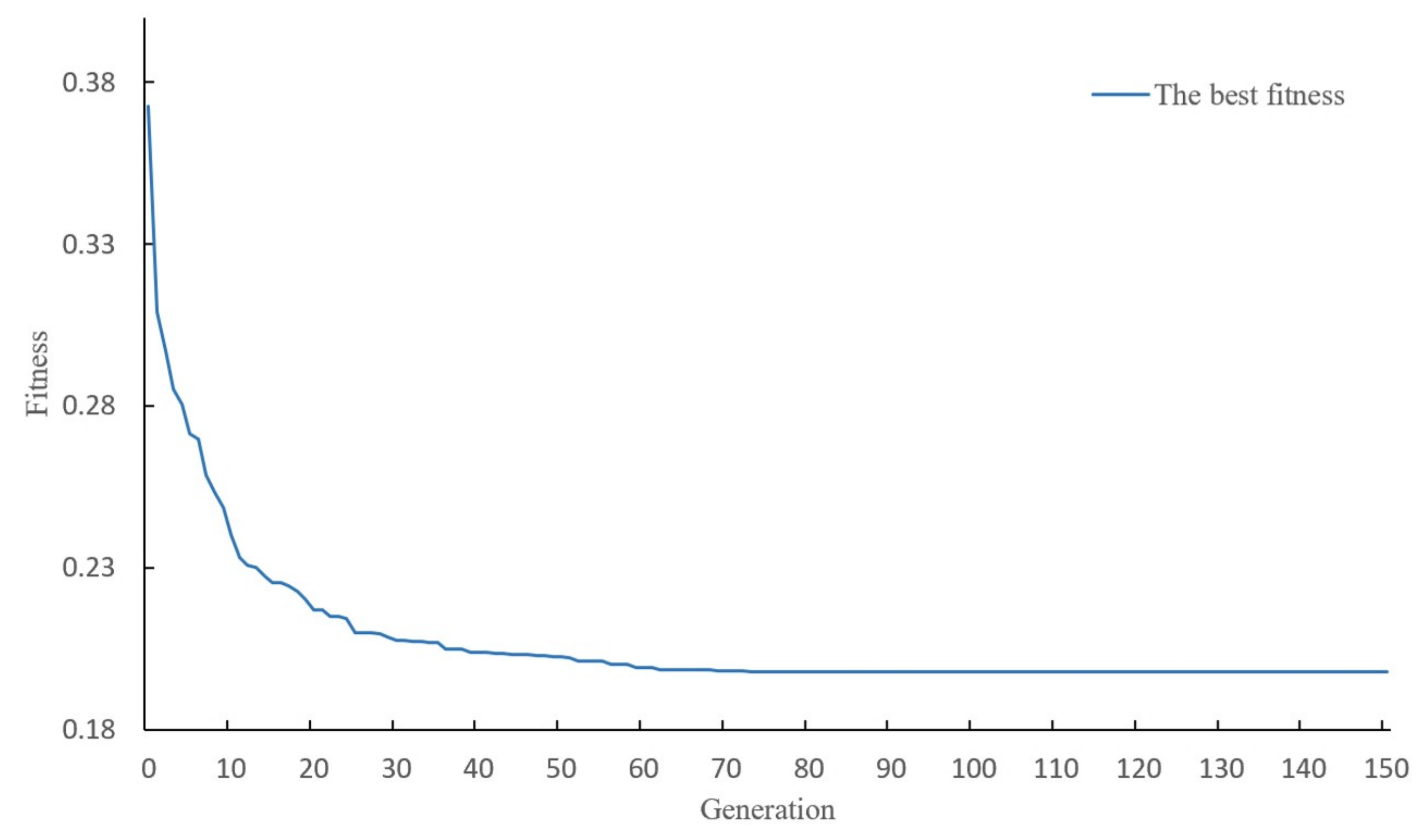
5.1. The Evolution Efficiency of SCA

When we use ICEEMDAN to decompose daily crude oil price series and RVFL to build the prediction model, we need to set a variety of parameters for these algorithms in advance. Since these parameters greatly impact the performance of prediction model, the parameter optimization is very important. In this study, we use the powerful global search ability of SCA to obtain the optimum parameter settings for ICEEMDAN and RVFL. To evaluate the evolution efficiency of SCA for parameter optimization, we set 50 and 150 as the fixed population size and the max number of evolution generations respectively, and execute ICEEMDAN-SCA-RVFL for crude oil price forecasting. The variation of the best fitness value (RMSE) with generations is shown in Figure 4.

As shown in this figure, the value of the best fitness gradually decreases when generation increases from 1 to 80, showing that the forecasting precision continuously improves with the evolution of SCA. However, when the number of generation is greater than 80, the value of best fitness tends to be roughly stable, indicating that SCA has already found the optimum solution. The result shows that SCA has powerful search ability and can efficiently obtain the optimum parameters settings for ICEEMDAN and RVFL within a relatively small number of generations.

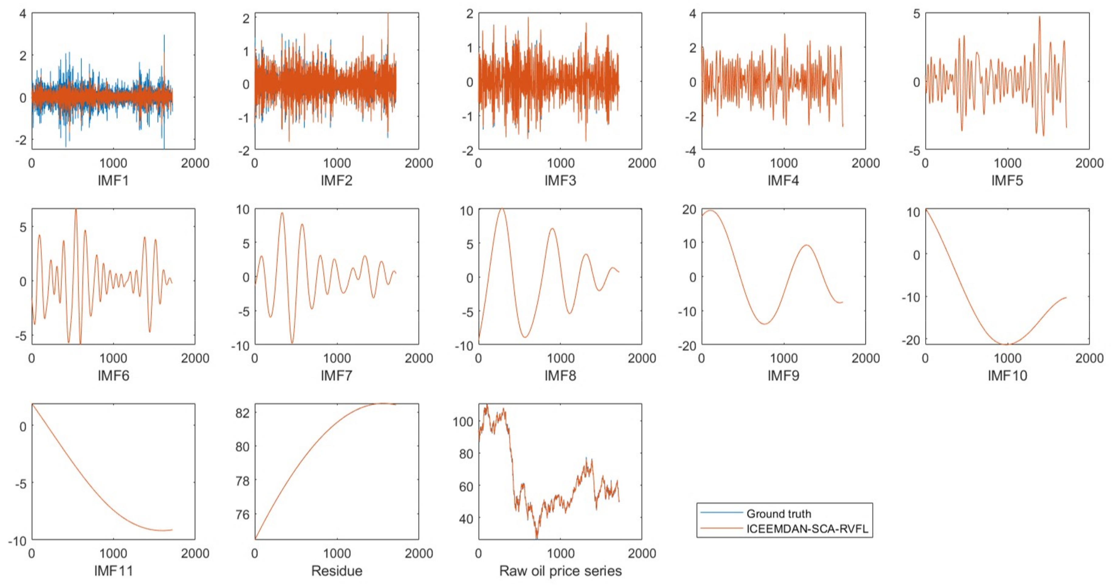
5.2. The Prediction Result of Each Individual Component

In the proposed ICEEMDAN-SCA-RVFL model, the prediction model of SCA-RVFL is constructed on each decomposed component independently, and then each prediction model is applied to the corresponding test data set. It can be seen from Figure 3 that the decomposed components demonstrate the distinct characteristics: high-frequency or low-frequency. In general, the first several decomposed components contains more high-frequency signals, while the last ones mainly involve low-frequency characteristics. Compared with the low-frequency components, it is more difficult to forecast the high-frequency ones accurately owning to their dramatic fluctuations. The real values and the predicted values of each component by SCA-RVFL, as well as the real raw crude oil prices and the final ensemble predicted results with Horizon 1 are shown in Figure 5.

Figure 5 shows that SCA-RVFL is capable of accurately forecasting the low-frequency components (IMF6–IMF11, and the residue), and the main prediction errors are caused by the dramatic fluctuations of the high-frequency components (IMF1–IMF5).

Table 8. Prediction results of each decomposed component.

Tested Model	Component	RMSE	MAPE	Dstat
	IMF1	0.2885	3.6136	0.8493
	IMF2	0.1119	1.1606	0.9221
	IMF3	0.0136	0.4906	0.9820
	IMF4	0.0019	0.0075	0.9971
	IMF5	0.0003	0.0017	1.0000
ICEEMDAN-SCA-RVFL	IMF6	$\mathbf{2.1130}\times {\mathbf{10}}^{-\mathbf{5}}$	$\mathbf{5.4234}\times {\mathbf{10}}^{-\mathbf{5}}$	1.0000
	IMF7	$\mathbf{1.5799}\times {\mathbf{10}}^{-\mathbf{6}}$	$\mathbf{2.4054}\times {\mathbf{10}}^{-\mathbf{6}}$	1.0000
	IMF8	$\mathbf{1.6047}\times {\mathbf{10}}^{-\mathbf{7}}$	$\mathbf{1.2096}\times {\mathbf{10}}^{-\mathbf{7}}$	1.0000
	IMF9	$\mathbf{9.3338}\times {\mathbf{10}}^{-\mathbf{7}}$	$5.6325\times {10}^{-7}$	1.0000
	IMF10	$4.6501\times {10}^{-6}$	$\mathbf{2.1335}\times {\mathbf{10}}^{-\mathbf{6}}$	1.0000
	IMF11	$4.5926\times {10}^{-6}$	$\mathbf{2.2972}\times {\mathbf{10}}^{-\mathbf{6}}$	1.0000
	Residue	$\mathbf{9.2626}\times {\mathbf{10}}^{-\mathbf{7}}$	$\mathbf{1.2012}\times {\mathbf{10}}^{-\mathbf{8}}$	0.9994
	Raw oil price series	0.2801	0.0035	0.9273
	IMF1	0.3192	4.4029	0.8307
	IMF2	0.1141	1.8793	0.9157
	IMF3	0.0147	0.4197	0.9848
	IMF4	0.0021	0.01579	0.9948
	IMF5	0.0003	0.0010	1.0000
ICEEMDAN-RVFL	IMF6	$2.6587\times {10}^{-5}$	$9.6048\times {10}^{-5}$	1.0000
	IMF7	$2.0455\times {10}^{-6}$	$2.4358\times {10}^{-6}$	1.0000
	IMF8	$5.4683\times {10}^{-7}$	$7.9149\times {10}^{-7}$	1.0000
	IMF9	$1.4726\times {10}^{-7}$	$\mathbf{8.3568}\times {\mathbf{10}}^{-\mathbf{8}}$	1.0000
	IMF10	$\mathbf{4.1368}\times {\mathbf{10}}^{-\mathbf{6}}$	$2.6351\times {10}^{-6}$	1.0000
	IMF11	$\mathbf{4.4277}\times {\mathbf{10}}^{-\mathbf{6}}$	$1.2113\times {10}^{-5}$	1.0000
	Residue	$2.0173\times {10}^{-6}$	0.0001	0.9779
	Raw oil price series	0.3187	0.0040	0.9186

shows the values of RMSE, MAPE, and Dstat of the predicted results of each component by SCA-RVFL and RVFL, respectively. From this table, we can find that the RMSE and MAPE values of the high-frequency components are much higher than those of the low-frequency ones, further indicating that the final ensemble error mainly comes from the prediction of first several components.

Furthermore, as for RMSE, ICEEMDAN-SCA-RVFL is superior to ICEEMDAN-RVFL in all the components except IMF10 and IMF11, while as for MAPE, the former outperforms the latter except IMF3 and IMF9. In summary, SCA-RVFL outperforms RVFL in most of component predictions, showing SCA is able to search optimum parameters for RVFL and then significantly improve individual component predictions.

6. Conclusions

Accurately forecasting crude oil prices is an important but challenging task. For the purpose of better forecasting crude oil prices, this paper develops a novel self-optimizing ensemble learning paradigm (ICEEMDAN-SCA-RVFL) incorporating ICEEMDAN, SCA, and RVFL. The proposed ICEEMDAN-SCA-RVFL model first uses ICEEMDAN to decompose the raw crude oil price series into a group of components, and then each decomposed component is individually forecasted using RVFL predictors. In the decomposition and individual forecasting stages, SCA is employed to optimize the parameter settings of both ICEEMDAN and RVFL to further enhance the prediction performance. Finally, the predicted results of individual components are aggregated as the final forecasting results using addition. To the best of our knowledge, this is the first time that SCA is applied to the parameter optimization for ICEEMDAN and RVFL in crude oil price forecasting.

The experimental results demonstrate that: (1) compared with benchmark models, our proposed ICEEMDAN-SCA-RVFL is able to significantly enhance the prediction performance for crude oil price forecasting; (2) ICEEMDAN outperforms EEMD for decomposing raw crude oil price series; and (3) SCA can efficiently search the optimum parameters for ICEEMDAN and RVFL, which contributes to improving prediction performance of crude oil prices.

The main advantage of the proposed ICEEMDAN-SCA-RVFL is that it makes full use of the respective advantages of ICEEMDAN, SCA, and RVFL, and can greatly improve the prediction performance for crude oil price forecasting compared with some state-of-the-art prediction models. On the other hand, since the predictor RVFL is a kind of typical neural network, the ensemble forecasting model has relatively poor interpretability compared with traditional regression models. In addition, we use SCA to search the optimum parameter settings for ICEEMDAN and RVFL in this study, so the whole execution time of the proposed model is relatively longer than that of other forecasting models using fixed parameters. Totally, despite the disadvantages, our proposed ICEEMDAN-SCA-RVFL significantly enhances the prediction performance, showing it is promising for crude oil price forecasting.

From the perspective of the input of the forecasting task, crude oil price forecasting can be divided into two categories: multivariate forecasting and univariate forecasting. The former usually uses a variety of data, such as macroeconomic variables, sentiment analysis, inventory variables, previous crude oil prices, and so on, to develop predictors, while the latter only uses the previous oil prices. The current study belongs to the latter. In the future, we will extend our work in three aspects: (1) developing a novel multivariate forecasting model for crude oil price prediction; (2) applying SCA to optimize more decomposition and prediction approaches for forecasting crude oil prices; and (3) using other time series of energy to further evaluate the ICEEMDAN-SCA-RVFL model.

References

1. Zhao, Y.; Li, J.; Yu, L. A deep learning ensemble approach for crude oil price forecasting. Energy Econ. 2017, 66, 9–16. [Google Scholar] [CrossRef]
2. Zhu, B.; Shi, X.; Chevallier, J.; Wang, P.; Wei, Y.M. An adaptive multiscale ensemble learning paradigm for nonstationary and nonlinear energy price time series forecasting. J. Forecast. 2016, 35, 633–651. [Google Scholar] [CrossRef]
3. Wu, J.; Chen, Y.; Zhou, T.; Li, T. An adaptive hybrid learning paradigm integrating CEEMD, ARIMA and SBL for crude oil price forecasting. Energies 2019, 12, 1239. [Google Scholar] [CrossRef] [Green Version]
4. Lanza, A.; Manera, M.; Giovannini, M. Modeling and forecasting cointegrated relationships among heavy oil and product prices. Energy Econ. 2005, 27, 831–848. [Google Scholar] [CrossRef]
5. e Silva, E.G.d.S.; Legey, L.F.; e Silva, E.A.d.S. Forecasting oil price trends using wavelets and hidden Markov models. Energy Econ. 2010, 32, 1507–1519. [Google Scholar] [CrossRef]
6. Xiang, Y.; Zhuang, X.H. Application of ARIMA model in short-term prediction of international crude oil price. Adv. Mater. Res. Trans. Tech. Publ. 2013, 798, 979–982. [Google Scholar] [CrossRef]
7. Wei, Y.; Wang, Y.; Huang, D. Forecasting crude oil market volatility: Further evidence using GARCH-class models. Energy Econ. 2010, 32, 1477–1484. [Google Scholar] [CrossRef]
8. Ramyar, S.; Kianfar, F. Forecasting crude oil prices: A comparison between artificial neural networks and vector autoregressive models. Comput. Econ. 2019, 53, 743–761. [Google Scholar] [CrossRef]
9. Mirmirani, S.; Li, H.C. A comparison of VAR and neural networks with genetic algorithm in forecasting price of oil. Adv. Econometr. 2004, 19, 203–223. [Google Scholar]
10. Bashiri Behmiri, N.; Pires Manso, J.R. Crude oil Price Forecasting Techniques: A Comprehensive Review of Literature. Altern. Invest. Anal. Rev. 2013, 2, 30–49. [Google Scholar] [CrossRef]
11. Mostafa, M.M.; El-Masry, A.A. Oil price forecasting using gene expression programming and artificial neural networks. Econ. Model. 2016, 54, 40–53. [Google Scholar] [CrossRef] [Green Version]
12. Kulkarni, S.; Haidar, I. Forecasting model for crude oil price using artificial neural networks and commodity futures prices. arXiv 2009, arXiv:0906.4838. [Google Scholar]
13. Xie, W.; Yu, L.; Xu, S.; Wang, S. A new method for crude oil price forecasting based on support vector machines. In Proceeding of the International Conference on Computational Science, Reading, UK, 28–31 May 2006; pp. 444–451. [Google Scholar]
14. Shu-rong, L.; Yu-lei, G. Crude oil price prediction based on a dynamic correcting support vector regression machine. Abstr. Appl. Anal. 2013, 2013, 528678. [Google Scholar] [CrossRef]
15. Li, T.; Hu, Z.; Jia, Y.; Wu, J.; Zhou, Y. Forecasting crude oil prices using ensemble empirical mode decomposition and sparse Bayesian learning. Energies 2018, 11, 1882. [Google Scholar] [CrossRef] [Green Version]
16. Wang, J.; Athanasopoulos, G.; Hyndman, R.J.; Wang, S. Crude oil price forecasting based on internet concern using an extreme learning machine. Int. J. Forecast. 2018, 34, 665–677. [Google Scholar] [CrossRef]
17. Gumus, M.; Kiran, M.S. Crude oil price forecasting using XGBoost. In Proceedings of the 2017 International Conference on Computer Science and Engineering (UBMK), Antalya, Turkey, 5–7 October 2017; pp. 1100–1103. [Google Scholar]
18. Tang, L.; Wu, Y.; Yu, L. A non-iterative decomposition-ensemble learning paradigm using RVFL network for crude oil price forecasting. Appl. Soft Comput. 2018, 70, 1097–1108. [Google Scholar] [CrossRef]
19. Mingming, T.; Jinliang, Z. A multiple adaptive wavelet recurrent neural network model to analyze crude oil prices. J. Econ. Bus. 2012, 64, 275–286. [Google Scholar] [CrossRef]
20. Yu, L.; Dai, W.; Tang, L.; Wu, J. A hybrid grid-GA-based LSSVR learning paradigm for crude oil price forecasting. Neural Comput. Appl. 2016, 27, 2193–2215. [Google Scholar] [CrossRef]
21. Chen, Y.; Zhang, C.; He, K.; Zheng, A. Multi-step-ahead crude oil price forecasting using a hybrid grey wave model. Phys. A Stat. Mech. Appl. 2018, 501, 98–110. [Google Scholar] [CrossRef]
22. Wang, S.; Yu, L.; Lai, K.K. A novel hybrid AI system framework for crude oil price forecasting. In Proceedings of the Chinese Academy of Sciences Symposium on Data Mining and Knowledge Management, Beijing, China, 12–14 July 2004; pp. 233–242. [Google Scholar]
23. Tehrani, R.; Khodayar, F. A hybrid optimized artificial intelligent model to forecast crude oil using genetic algorithm. Afr. J. Bus. Manag. 2011, 5, 13130. [Google Scholar] [CrossRef]
24. Li, T.; Zhou, Y.; Li, X.; Wu, J.; He, T. Forecasting daily crude oil prices using improved CEEMDAN and ridge regression-based predictors. Energies 2019, 12, 3603. [Google Scholar] [CrossRef] [Green Version]
25. Zhou, Y.; Li, T.; Shi, J.; Qian, Z. A CEEMDAN and XGBOOST-based approach to forecast crude oil prices. Complexity 2019, 2019, 4392785. [Google Scholar] [CrossRef] [Green Version]
26. Li, T.; Qian, Z.; He, T. Short-term Load Forecasting with Improved CEEMDAN and GWO-based Multiple Kernel ELM. Complexity 2020, 2020, 1209547. [Google Scholar] [CrossRef]
27. Wu, J.; Zhou, T.; Li, T. Detecting Epileptic Seizures in EEG Signals with Complementary Ensemble Empirical Mode Decomposition and Extreme Gradient Boosting. Entropy 2020, 22, 140. [Google Scholar] [CrossRef] [Green Version]
28. Bao, Y.; Zhang, X.; Yu, L.; Lai, K.K.; Wang, S. An integrated model using wavelet decomposition and least squares support vector machines for monthly crude oil prices forecasting. New Math. Natural Comput. 2011, 7, 299–311. [Google Scholar] [CrossRef]
29. He, K.; Zha, R.; Wu, J.; Lai, K.K. Multivariate EMD-based modeling and forecasting of crude oil price. Sustainability 2016, 8, 387. [Google Scholar] [CrossRef] [Green Version]
30. Li, T.; Zhou, M.; Guo, C.; Luo, M.; Wu, J.; Pan, F.; Tao, Q.; He, T. Forecasting crude oil price using EEMD and RVM with adaptive PSO-based kernels. Energies 2016, 9, 1014. [Google Scholar] [CrossRef] [Green Version]
31. Liu, H.; Wu, H.; Li, Y. Smart wind speed forecasting using EWT decomposition, GWO evolutionary optimization, RELM learning and IEWT reconstruction. Energy Convers. Manag. 2018, 161, 266–283. [Google Scholar] [CrossRef]
32. Huang, N.E.; Shen, Z.; Long, S.R.; Wu, M.C.; Shih, H.H.; Zheng, Q.; Yen, N.C.; Tung, C.C.; Liu, H.H. The empirical mode decomposition and the Hilbert spectrum for nonlinear and non-stationary time series analysis. Proc. R. Soc. Lond. Ser. A Math. Phys. Eng. Sci. 1998, 454, 903–995. [Google Scholar] [CrossRef]
33. Wu, Z.; Huang, N.E. Ensemble empirical mode decomposition: A noise-assisted data analysis method. Adv. Adapt. Data Anal. 2009, 1, 1–41. [Google Scholar] [CrossRef]
34. Torres, M.E.; Colominas, M.A.; Schlotthauer, G.; Flandrin, P. A complete ensemble empirical mode decomposition with adaptive noise. In Proceedings of the 2011 IEEE International Conference on Acoustics, Speech and Signal Processing (ICASSP), Prague, Czech Republic, 22–27 May 2011; pp. 4144–4147. [Google Scholar]
35. Colominas, M.A.; Schlotthauer, G.; Torres, M.E. Improved complete ensemble EMD: A suitable tool for biomedical signal processing. Biomed. Signal Process. Control 2014, 14, 19–29. [Google Scholar] [CrossRef]
36. Hao, Y.; Tian, C.; Wu, C. Modelling of carbon price in two real carbon trading markets. J. Clean. Prod. 2020, 244, 118556. [Google Scholar] [CrossRef]
37. Yang, W.; Wang, J.; Niu, T.; Du, P. A hybrid forecasting system based on a dual decomposition strategy and multi-objective optimization for electricity price forecasting. Appl. Energy 2019, 235, 1205–1225. [Google Scholar] [CrossRef]
38. Khorramdel, B.; Azizi, M.; Safari, N.; Chung, C.; Mazhari, S. A Hybrid Probabilistic Wind Power Prediction Based on An Improved Decomposition Technique and Kernel Density Estimation. In Proceedings of the 2018 IEEE Power & Energy Society General Meeting (PESGM), Portland, OR, USA, 5–10 August 2018; pp. 1–5. [Google Scholar]
39. Mirjalili, S. SCA: A sine cosine algorithm for solving optimization problems. Knowl. Based Syst. 2016, 96, 120–133. [Google Scholar] [CrossRef]
40. Deng, W.; Liu, H.; Xu, J.; Zhao, H.; Song, Y. An improved quantum-inspired differential evolution algorithm for deep belief network. IEEE Trans. Instrum. Meas. 2020. [Google Scholar] [CrossRef]
41. Deng, W.; Zhao, H.; Yang, X.; Xiong, J.; Sun, M.; Li, B. Study on an improved adaptive PSO algorithm for solving multi-objective gate assignment. Appl. Soft Comput. 2017, 59, 288–302. [Google Scholar] [CrossRef]
42. Hekimoğlu, B. Sine-cosine algorithm-based optimization for automatic voltage regulator system. Trans. Inst. Meas. Control 2019, 41, 1761–1771. [Google Scholar] [CrossRef]
43. Majhi, S.K. An efficient feed foreword network model with sine cosine algorithm for breast cancer classification. Int. J. Syst. Dyn. Appl. 2018, 7, 1–14. [Google Scholar] [CrossRef] [Green Version]
44. Pao, Y.H.; Takefuji, Y. Functional-link net computing: Theory, system architecture, and functionalities. Computer 1992, 25, 76–79. [Google Scholar] [CrossRef]
45. Igelnik, B.; Pao, Y.H. Stochastic choice of basis functions in adaptive function approximation and the functional-link net. IEEE Trans. Neural Netw. 1995, 6, 1320–1329. [Google Scholar] [CrossRef] [Green Version]
46. Aggarwal, A.; Tripathi, M. Short-term solar power forecasting using random vector functional link (RVFL) network. In Ambient Communications and Computer Systems; Springer: Singapore, 2018; pp. 29–39. [Google Scholar]
47. Li, T.; Shi, J.; Li, X.; Wu, J.; Pan, F. Image encryption based on pixel-level diffusion with dynamic filtering and DNA-level permutation with 3D Latin cubes. Entropy 2019, 21, 319. [Google Scholar] [CrossRef] [Green Version]
48. Wu, J.; Shi, J.; Li, T. A novel image encryption approach based on a hyperchaotic system, pixel-level filtering with variable kernels, and DNA-level diffusion. Entropy 2020, 22, 5. [Google Scholar] [CrossRef] [Green Version]
49. Li, T.; Yang, M.; Wu, J.; Jing, X. A novel image encryption algorithm based on a fractional-order hyperchaotic system and DNA computing. Complexity 2017, 2017, 9010251. [Google Scholar] [CrossRef] [Green Version]
50. Li, X.; Xie, Z.; Wu, J.; Li, T. Image encryption based on dynamic filtering and bit cuboid operations. Complexity 2019, 2019, 7485621. [Google Scholar] [CrossRef]
51. Zhao, H.; Liu, H.; Xu, J.; Deng, W. Performance prediction using high-order differential mathematical morphology gradient spectrum entropy and extreme learning machine. IEEE Trans. Instrum. Meas. 2019. [Google Scholar] [CrossRef]
52. Qiu, X.; Suganthan, P.N.; Amaratunga, G.A. Electricity load demand time series forecasting with empirical mode decomposition based random vector functional link network. In Proceedings of the 2016 IEEE International Conference on Systems, Man, and Cybernetics (SMC), Budapest, Hungary, 9–12 October 2016; pp. 001394–001399. [Google Scholar]
53. Ren, Y.; Suganthan, P.N.; Srikanth, N.; Amaratunga, G. Random vector functional link network for short-term electricity load demand forecasting. Inf. Sci. 2016, 367, 1078–1093. [Google Scholar] [CrossRef]
54. EIA Website. Available online: https://www.eia.gov/dnav/pet/hist/rwtcD.htm (accessed on 14 February 2020).
Figure 1. Architecture of RVFL. RVFL: Random vector functional link neural network.
Energies 13 01852 g001
Figure 2. The flowchart of the proposed ICEEMDAN-SCA-RVFL. ICEEMDAN: Improved complete ensemble empirical mode decomposition with adaptive noise; SCA: Sine cosine algorithm; RVFL: Random vector functional link neural network.
Energies 13 01852 g002
Figure 3. The crude oil prices and the corresponding decomposed components by ICEEMDAN. ICEEMDAN: Improved complete ensemble empirical mode decomposition with adaptive noise.
Energies 13 01852 g003
Figure 4. The best fitness of SCA.
Energies 13 01852 g004
Figure 5. Individual prediction result of each component and ensemble prediction result by ICEEMDAN-SCA-RVFL.
Energies 13 01852 g005